Open Journal Systems

Hungarian Association of Agricultural Informatics European Federation for Information Technology in Agriculture, Food and the Environment

Journal of Agricultural Informatics. Vol. 9, No. 2

journal.magisz.org

Application of the multiple objective programming in the optimization of

production structure of an agricultural holding

Lajos Nagy1_{, László Pusztai}2_{, Margit Csipkés}3

I N F O

Received 2 Mar 2018 Accepted 7 May 2018 Available on-line 18 Jun 2018 Responsible Editor: M. Herdon

Keywords:

linear programminf, MOLP, agricultural, sequential programming.

A B S T R A C T

At an agricultural plant during the preparation of the annual plan, besides taking resources as well as market opportunities into account, we wish to accomplish a production structure which can provide maximum income for the company. As an effect of climate change extreme weather conditions can be experienced more frequently than before, which conditions are tolerated in different ways by arable cultures with variable terrain features. When there is an agreement in the final production structure, decision makers take even risk factors into account in their decision making. Endeavour for reducing burden on the environment is playing a more and more important role in decision making. These endeavors are often of opposite directions but they can be coordinated as well as compromises can be found by the application of multiple objective programming. In our article we aim at introducing opportunities for the application of this method.

1. Introduction

Optimization is generally carried out by aiming at only one goal in programming models (Winston 1997). In economic models the most common goals are either those of maximizing income or minimizing costs. In some cases, however, the decision maker needs to set up more than one different goals simultaneously. For instance, a manufacturing company would like to focus on utilizing their available resources in the most efficient ways, which requires achieving several and counteractive goals at the same time. For instance, when a company would like to reach, several, opposing goals at a time. Such counteractive goals are those of maximizing income and minimizing cost parallelly. Furthermore, a small- and medium sized company can have social political goals as well in order to provide a relatively high employment ratio integrated with the two previous goals. In order to protect the environment, the reduction of pollutant emission, the increase in the level of customer service, - and the list could be further expanded -, are all important goals in a company’s life, but these goals can be counteractive in both simple or complicated ways. The harmonization of these different goals is not always an easy task because the quantificated values of these goals can be one of the sources for a company’s competitiveness (Ragsdale 2007).

Multiple objective programming is widely applied in the field of economics and finance, in the optimization of production processes as well as production structure optimization and in many other fields of life. The applied methods are also quite diverse as a wide range of operations research methods are applied in solving different problems.

Multiple objective programming was applied to solve site location problems (Scheiderjans et al. 1982) or snow removal work in Montreal was modelled by Cambell & Langevin (1995). Chih and

1 _{Lajos Nagy}

University of Debrecen [email protected]

2 _{László Pusztai}

University of Debrecen [email protected]

3 _{Margit Csipkés}

University of Debrecen

Ching (1996) applied multiple objective programming to create water quality management. Agricultural applications are also quite widespread: Tóth & Szenteleki published their work on compromise programming in 1983. However, we can read about agricultural research in the field of cattle breeding (Mendez et al. 1988), in regional agricultural forecast (Zekri & Romero 1992), as well as in vegetable production (Berber et al. 1991). Risk programming models combine the elements of linear programming or quadratic programming with those of game theory to resolve conflicts between profitability and risk as well as to select the compromise most suitable for the decision maker (Hazell 1971; Hazell & Norton 1986; Hardaker et al. 1997; Berbel 1993).

In our article, we look for answers to whether a plant-growing enterprise can successfully use multi-purpose programming at decision-making. We review basic model types, present a real-life practical application, and provide suggestions on how to implement and choose models.

2. Multiple Objective Linear Programming models (MOLP)

Numerous papers have been published on several versions and algorithms of multi objective programming. Article written in 2015 by Colapito et al. provides a detailed overview and summary about the emergence and evolution of models as well as their applicability in different professional fields.

In this chapter we are going to introduce the basic types of the above mentioned models, and their role in analyses. We are going to deal with goal programming and MOLP model in detail, because it was these methods that we applied to determine the optimal production structure with regard to multiple targets at an agricultural plant.

2.1. General determination and justification of the model

value t coefficien objective c optimum x c optimum x c confine b b x a need specific a b x a ied x b x a n j x kj j j j

j kj j

i

j ij j i

ij

j ij j i

j

j ij j i

j : : : var : ,.. 3 , 2 , 1 0 ' ' 2 ' = = = ≥ ≤ = ≥

∑

∑

∑

∑

∑

K K K K K K K

In the general model we set the constraints as well as the goals preferred by the decision maker. In case of contradictory goals (e.g. cost reduction and maximum income achievement), the enhancement of one goal will entail the enhancement of the other, which may not be desirable. For example, in particular areas, such as the different branches of plant cultivation as well as in the selection of farming intensity, apart from profitability aspects, expenses play an important role as well, especially in case of less capital-intensive farming companies. Therefore, regarding goals, producers have to make compromises taking their circumstances into account.

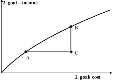
Compromises are a necessary part of the decision making process, however, in case of conventional planning it is not easy to find a solution, which results in making only minimal concessions in the goals (Figure 1).

target income, the second target value (point B) is higher, than the first target value (A). As a consequence, solutions A and B always dominate over C.

Figure 1. Compromise decisions – dominant and non-dominant versions (Source: Own editing

according to Ragsdale, 2007)

Multi objective programming can guarantee non-dominant solutions and it enables to make decisions at system level. Every solution in the trade-off curve section between A and B is Pareto-optimal.

2.2. Modelling opportunities in case of multiple objectives

2.2.1. Alternative programs

Alternative programming can be applied when a compromise solution is calculated between two, one directional goals (Chiandussi 2012). One of our goals can be the achievement of maximal gross margin, the other can be the achievement of maximal net income. The method is quite simple. First of all, the linear programming model is solved on the basis of the first, then of the second objective. In case different optimal values are calculated, the programs can be combined with distribution ratios (Table 1).

Table 1. Compromise solution determination with the use of alternative linear programming

Optimum 1.

objective

Optimum 2.

objective

Compromise

V

ar

iab

le

s

x

1opt1

x

1opt2

k

1

x

1opt1

+k

2

x

1opt2

x

2opt1

x

2opt2

k

1

x

2opt1

+k

2

x

2opt2

…

…

x

mopt1

x

mopt2

k

1

x

mopt1

+k

2

x

mopt2

z

1

max

z

1opt1

z

1opt2

k

1

z

1opt1

+k

2

z

1opt2

z

2

max

z

2opt1

z

2opt2

k

1

z

2opt1

+k

2

z

2opt2

Distribution

ratios

k

1

k

2

k

1

+k

2

=1

B

A

C

2.2.2. Sequential programming

In case of sequential programming we rank goals according to their importance. Optimization is started with the most important goal: f x₁( )=

∑

_jc'₁j xj, with an

L

1 solution set. Subsequently,

optimization with the remaining goals is carried out in accordance with the obtained importance rank to get

L L

₂

,

₃

,...

L

_msolution sets. If there is a common L, which is true for

L

⊂

L

_m−1

⊂ ⊂

...

L

₂

⊂

L

₁, it means that all the objective functions have their own optimum value within the Lsolution set, otherwise all the goals cannot be optimized simultaneously.

The method is quite simple. Although its efficiency is questionable, it definitely has at least two advantages. On the one hand, goals with similar optimum values can be identified, which makes it possible to reduce the number of objective functions for further analysis. On the other hand, marginal values of objective functions (e.g. resources, market conditions, etc.) can be revealed and it plays an important role in further examinations (Benayoun et al. 1970).

2.2.3. Constraints programming

The most important goal will be the objective of this model, all the other goals are considered as constraints,

p

_iconstant is on the right side of the equation. These constants are between the

predetermined minimal (

m

_i) and maximal (

M

_i) goal values (

m

_i

≤

p

_i

≤

M

_i). Objective function

values of secondary goals acquired by sequential programming can provide a useful point of reference for the determination of

p

i.

The model:

1 1

2 2

0

1, 2, 3...

'

'

'

'

j

ij j i j

ij j i j

ij j i j

j j j

j j j

kj j k j

főcél j j j

x

j

n

a x

b

a x

b

a x

b

c

x

p

c

x

p

c

x

p

c

x

extrém

≥

=

≤

≥

=

=

=

=

− − − − − − − − −

→

∑

∑

∑

∑

∑

∑

∑

M

In case of secondary goals, the relations are not necessarily equalities. There can be either

≤

(minimal goals) or

≥

(maximum goals). With this method our main goals within the given restrictions will be definitely accomplished, in case of all the other goals - with regard to deviations from them - we can carry out further research through sensitivity analysis (Marler & Arora 2004).

2.2.4. Goal programming

Instead of objective functions, we insert equations with predetermined goal values into the constraints. The objective function minimalizes the sum of negative or positive deviations from the targeted values. Constraints regarding goals:

k k k j kj j i i i j ij j j j j t d d x c t d d x c t d d x c d d = − + = − + = − + ≥ ≥ + − + − + − + −

∑

∑

∑

' ' ' 0 , 0 1 1 1 1 1 1 M

The objective function:

i i

id d MINIMUM

−₊ +_→

∑

Function no. 4. can be used when the measure unit of goals are identical and when there are not disturbing differences between their quantities. On the contrary, it is practical to calculate with the relative deviation from the targeted goal that can be expressed in percentages:

1

(

_{i i}

)

i

i

d

d

MINIMUM

t

−

₊

+

_→

∑

The question arises as to how individual goals can be ordered on the basis of their importance, because there can be goals, whose deviations from the target goal lead to bigger differences. In this case weights can be added to deviation variables:

MINIMUM d w d w t or MINIMUM d w d w i i i i i i i i i i i → + → + + + − − + + − −

∑

∑

) ( 1 ) (

By applying goal programming, the fine adjustment of different goals can be made possible. By using weights, one or more goals can be highlighted, and the decision maker will have the opportunity to find the most appropriate compromise solution (Ragsdale, 2007).

2.2.5. MOLP – Multiple objective linear programming

With the use of goal programming we searched for such a compromise solutions, where the total deviation from goals were minimal. MOLP method provides us another solution. In this case, the goal is to find the minimal value of the deviation from individual goals. First of all, deviations from individual goals must be calculated:

'_{ij j i} j

i

c x t t

−

∑

This can be weighted in accordance with their importance, like in the case of goal programming:

'

_{ij j i} j

i

i

c

x

t

w

t



−















∑

Q

minimax variable was implemented, which is constraints as well. Thus, the objective function of the model:

Q

→

MINIMUM

which has the following constraint:

'

ij j i j

i

i

c

x

t

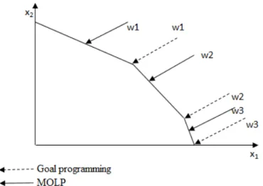
According and optimal solution can be calculated, where the maximum deviation from individual goals is the lowest. With this method fault can be avoided that the total deviation is minimal, but there are poorly-performing objectives, which are common in goal programming (Winston 1997). The question can arise: whether the usage of goal programming or MOLP is more expedient? There is no exact answer for this question, but it is a fact, that results calculated with goal programming are belongs to an extremal point, while the results of MOLP is not in every case. This can usually result in that the deviation from individual goals is lower when using MOLP, so this can mean a good estimation (Figure 2).

Figure 2. Solutions acquired by goal programming and MOLP with the use of different weights

3. Production ratio optimization at a crop producer in Hajdúság based on several

objectives

The company in target utilizes a 2000-acre farming area: they produce winter wheat, corn, oilseeds (like sunflower, rape) and in irrigated areas they grow peas as well. Thus the variables of the model are: corn (x1), sunflower (x2), winter wheat (x3), rape (x4) and peas (x5). The production ratio is

optimized considering the following objectives: Revenue, Income, Sectoral result per 100 HUF production cost and Production cost. Objective factors are shown in Table 2.

Crop rotation conditions were considered as constraints in the model. Corn can be produced in the same area after every second year, while sunflower, rape and peas can be grown in the same soil only after every fifth year. Wheat can occupy maximum 60% of the total production area. The capacity of irrigation is 250 hectares. Regarding machines, professional work and unskilled work, the specific resource requirements were determined based on decade-specific technologies, while the amount of resources accessible in certain periods was given in hours.

Table 2. Sectoral indicators related to targeted objectives

Objectives Corn Sunflower Winter

wheat Rape Peas

Revenue (HUF/hectare) 436 800 230 000 266 900 378 000 684 000

Income (HUF/hectare) 152 750 103 632 82 096 136 984 266 000

(Income per production cost)

x 100 45.73 58.76 34.96 47.07 56.84

Production cost

The following model variants were calculated and evaluated:

•

Sequential programming

The models were calculated for each objective separately. There were two reasons to apply sequential programming. On the one hand, the possible extreme values and related optimal values for each objective were in the focus of the research. On the other hand, filtering common solution sets were also aimed at.

•

Goal programming

Goal programming model was calculated with both absolute and relative weights. The model’s objectives were those individual objectives which was calculated by sequential programming. 5 variants were calculated for each model. The difference between variant were in the importance weights of objectives. In the first variant, all objectives has the same weight. In the cases of the following variants production cost objective was get higher weights, which means that in the case of fifth variant, the weight become 5.

•

MOLP model

During the calculation of deviations from the goals, the extreme values acquired by sequential programming were used, and we assigned weight in accordance with the focus on the comparability with the results of goal programming.

2.3.

Results of sequential programming

During sequential programming 4 model variants were created. The model variants differed from one another with respect to the highlighted objectives (Table 3).

Table 3. Model variants

Name of the variant Highlighted objectives

Sz1 Maximum revenue

Sz2 Maximum income

Sz3 Maximum (income per production cost) x 100

Sz4 Minimum production cost

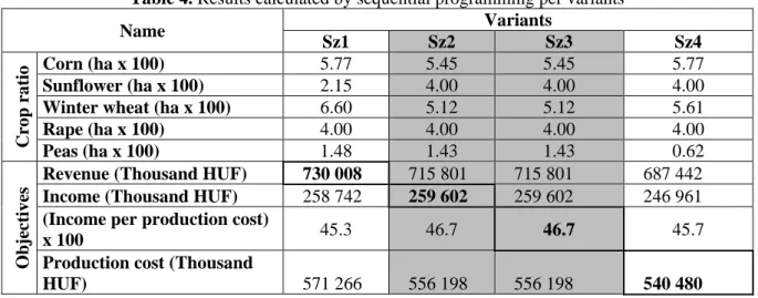
In the cases of Sz2 and Sz3 variants, programs and objectives are the same, so the second (income) and the third ((Income per production cost) x 100) objectives can be optimized at the same time (Table 4). Therefore, the third objective (income per 100 HUF production cost) is excluded from goal programming and MOLP models.

Table 4. Results calculated by sequential programming per variants

Name Variants

Sz1 Sz2 Sz3 Sz4

Cro

p

ra

ti

o

Corn (ha x 100) 5.77 5.45 5.45 5.77

Sunflower (ha x 100) 2.15 4.00 4.00 4.00

Winter wheat (ha x 100) 6.60 5.12 5.12 5.61

Rape (ha x 100) 4.00 4.00 4.00 4.00

Peas (ha x 100) 1.48 1.43 1.43 0.62

O

b

ject

iv

es

Revenue (Thousand HUF) 730 008 715 801 715 801 687 442

Income (Thousand HUF) 258 742 259 602 259 602 246 961

(Income per production cost)

x 100 45.3 46.7 46.7 45.7

Production cost (Thousand

HUF) 571 266 556 198 556 198 540 480

largest production area (660 hectares) in the case of maximum revenue objective, while this result is 100 hectares less in the case of production cost objective, however, winter wheat takes up about 150-acre smaller area in the calculation of the maximum of sectoral result. In the case of the first and second objectives it is advisable to grow peas in almost the same size of areas (143 hectares), however, its cost claim reduces its competitiveness (62 hectares) (Table 4).

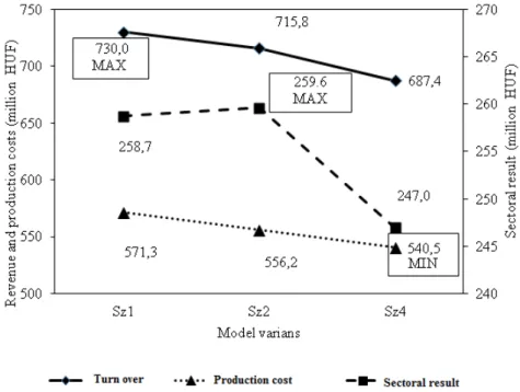
Figure 3. Objectives values calculated by sequential programming in the cases of different objectives

There is no significant difference between the sectoral result achieved at maximal revenue and the maximum sectoral result, however, the revenue related to the maximum sectoral result is approximately 15 million HUF less than the achievable maximum revenue. In the case of the achievable minimum cost, both the revenue and income decreased as expected (with 42.6 and 12.6 million HUF). Revenue loss in this case is 5.8%, result decrease is 4.8% compared to the maximum possible values

In the following we examined, what kind of opportunities are exist to search for compromise with the use of goal programming and MOLP. We considers available extreme values of goals as objectives.

2.4.

Evaluation of results acquired by goal programming and MOLP method

During goal programming, the models were calculated by using both relative and absolute weights. These models provided us the same results, therefore, in the comparison section only the relative weight results will be presented.

During calculation, for all objectives, deviations from the goal was taken into account with the same weights, then production cost was highlighted by penalty weights. Weights were increased from 1 to 5, and production cost as a goal is get bigger weights. These calculations were repeated in both goal programming and MOLP model. As a first step the results were compared, then the effects of increasing weight’s of production cost were evaluated.

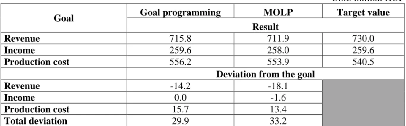
Table 5. Values and deviations calculated by goal programming and MOLP model

Unit: million HUF

Goal Goal programming MOLP Target value

Result

Revenue 715.8 711.9 730.0

Income 259.6 258.0 259.6

Production cost 556.2 553.9 540.5

Deviation from the goal

Revenue -14.2 -18.1

Income 0.0 -1.6

Production cost 15.7 13.4

Total deviation 29.9 33.2

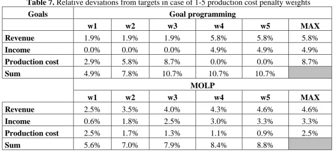
It is essential that the goals should not be in the same scale in absolute value, which means that using relative deviations could provide another picture. Based on the relative deviations from the targets, similar observations can be made as in the case of absolute deviations, that is, the higher difference there is between the revenue and the result of the MOLP model, the lower production cost there will be. There is a remarkable difference in Table 7. The total relative deviation is higher in the case of the MOLP model (Table 7, w1 column). The highest relative deviation can be identified in goal programming. This result was expected because in the objective of the MOLP model, the biggest relative deviation was minimized (Figure 4).

1,95%

0,00%

2,91%

2,48%

0,63%

2,48%

0% 1% 2% 3%

Revenue Sectoral results Prime cost

Goal programming Molp

Figure 4. Relative deviations from the goal in the cases of goal programming and MOLP method

Table 6. Production structure

Unit: hectare

Goal programming MOLP

Corn 545 522

Sunflower 400 400

Winter Wheat 512 535

Rape 400 400

Peas 143 143

The next step was the assignment of penalty weights to production costs. This means that production cost as a goal is becoming more and more important compared to other goals. The role of penalty weights is easy to understand, because in the case of goal programming, by increasing the weight from 1 to 2, w=2 being twice as much as in w=1 case, assuming the same production structure

.

As we search for the minimum of the total relative deviation, the optimal program will only be changed if the optimum belongs to another extremal point (Figure 2.) In the cases of goal programming, there is no change in w=1 and w=3 weights, only the linear increase of the relative deviation of production cost can be seen (2.9% →5.8%→8.7%). The deviation of the revenue and income did not change (1.9% and 0.0%). We experienced some changes with w=5 and w=6 weights. In this case, further increases in the weights would induce such a big change in the objective function that the optimal solution would belong to another extremal point.

In the case of the MOLP model it is revealed that with the increase of penalty weights, the total relative deviations will differ from. In the production cost, a slow decrease, while in the cases of the other two goals continuous increase can be detected (Table 7).

Table 7. Relative deviations from targets in case of 1-5 production cost penalty weights

Goals Goal programming

w1 w2 w3 w4 w5 MAX

Revenue 1.9% 1.9% 1.9% 5.8% 5.8% 5.8%

Income 0.0% 0.0% 0.0% 4.9% 4.9% 4.9%

Production cost 2.9% 5.8% 8.7% 0.0% 0.0% 8.7%

Sum 4.9% 7.8% 10.7% 10.7% 10.7%

MOLP

w1 w2 w3 w4 w5 MAX

Revenue 2.5% 3.5% 4.0% 4.3% 4.6% 4.6%

Income 0.6% 1.8% 2.5% 3.0% 3.3% 3.3%

Production cost 2.5% 1.7% 1.3% 1.1% 0.9% 2.5%

Sum 5.6% 7.0% 7.9% 8.4% 8.8%

Comparing the results of the two models in detail, the initial disadvantage of MOLP disappears with the increase of penalty weight, the total relative deviation is lower in the case of w=2, then goal programming. If we take the deviations from goals, MOLP seems more balanced.

Table 8. Change in production structure, in the cases of production cost penalty costs

Unit: hectare

Goal programming

w1 w2 w3 w4 w5

Corn 545 545 545 577 577

Sunflower 400 400 400 400 400

Winter wheat 512 512 512 561 561

Rape 400 400 400 400 400

Peas 143 143 143 62 62

MOLP

w1 w2 w3 w4 w5

Corn 522 507 523 533 540

Winter wheat 535 561 561 561 561

Rape 400 400 400 400 400

Peas 143 132 116 106 99

Optimal programs presented in table 8 verify the above statements. The goal programming basic model’s result (where the total weight is 1) equals with that solution, where sectoral result maximum was calculated. In the cases of those variants, where production cost penalty weights were w=4 and w=5 the optimal program is the same as sequential model, where the objective was the production cost. Changing the weight results in the selection of these two models.

In the cases of MOLP models, with the increase of the importance in production cost, tendencies in the production structure is similar like in the goal programming model. The production area of corn and winter wheat increases, the production area of peas decreases, while the areas of rape and sunflower are on the upper constraint in every variant. Optimal programs do not connect to extremal points, but all of them are on the trade-off curve.

3. Conclusion

In practice managers have to make decisions considering several objectives. One is more important than the other, nevertheless, none of these objectives should be excluded from the final decision making.

In the article some application opportunities and the importance of Multiple Objective Linear Programming methods are examined. The applicability of goal programming and that of MOLP were compared through an example of an agricultural enterprise.

It is suggested as a first step that the opportunities per goals be analyzed with the use of sequential programming. The calculated results can only provide information on single objectives, however, they can be applied during further examination. By using sequential programming, simultaneously optimizable objectives can be filtered, which can also help to make further examinations easier.

In the next step the application of both goal programming and MOLP models can be considered. In both models, we can represent the importance of high-priority goals with their assigned penalty weights. During our research, we have found that the goal programming model is less sensitive to the change in penalty weights than the MOLP model, so if the relative importance of our goals is different (for example, the priority of cost cutting is outstanding), it is more appropriate to use MOLP.

References

Benayoun R, de Montgolfier J, Tergny J & Laritchev O 1970, ‘Linear programming with multiple objective functions: Step method (stem)’ Mathematical Programming, Volume 1, Issue 1, pp. 366–375.

Berbel J 1993, ‘Risk programming in agricultural systems: A multiple criteria analysis’ Agricultural Systems, Volume 41, Issue 3, pp. 275-288. https://doi.org/10.1016/0308-521X(93)90004-L

Berbel J, Gallego J & Sagues H 1991, ‘Marketing goals vs. business profitability: An interactive multiple criteria decision-making approach’ Agribusiness,vol.7,issue 6, pp. 537-549. https://doi.org/10.1002/1520-6297(199111)7:6<537::AID-AGR2720070604>3.0.CO;2-D

Cambell J & Langevin A 1995, ‘The Snow Disposal Assigment Problem’ The Journal of the Operational Research Society. Vol 46. No.8. pp. 919-929. https://doi.org/10.1057/jors.1995.131

Chih-Sheng Lee & Ching-Gung Wen 1996, ‘Application of Multiobjective Programming to Water Quality Management in a River Basin’ Journal of Environmental Management. Vol. 47. Issue 1. pp. 11-26.

https://doi.org/10.1006/jema.1996.0032

Colapinto C, Jayaraman R & Marsiglio S 2015, ‘Multi-criteria decision analysis with goal programming in engineering, management and social sciences: a state-of-the art review’ Annals of Operations Research, Online First 1-34 (http://link.springer.com/article/10.1007%2Fs10479-015-1829-1)

Hazell PBR 1971, ‘A Linear Alternative to Quadratic and Semivariance Programming for Farm Planning Under Uncertainty’ American Journal of Agricultural Economics,vol.53. No. 1 pp. 53-62.

https://doi.org/10.2307/3180297

Hazell PBR & Norton RD 1986, ‘Mathematical Programming for Economic Analysis in Agriculture’ Macmillan Publishing Company, New York p.400

Hardaker JB, Huirne RBM & Anderson JR, 1997, ‘Coping with Risk in Agriculture’ CAB International, Wallingford p. xi + 274.

Hardaker JB, Richardson JW, Lien G & Schumann KD 2004, ‘Stochastic Efficiency Analysis with Risk Aversion Bounds: a Simplified Approach’ Australian Journal of Agricultural Economics pp. 253-270.

Marler RT & Arora JS 2004, ‘Survey of multi-objective optimization methods for engineering’ Structural and Multidisciplinary Optimization, Volume 26, Issue 6, pp. 369–395. https://doi.org/10.1007/s00158-003-0368-6

Mendez MM & Sebastian RA & Iruretagoyena Osuna TM 1988, ‘Cattle production systems by multiobjective programming for the tenth region of ChileAgricultural Systems’ vol. 28, issue 2, pp. 141-157.

Ragsdale, CT 2007, ‘Spreadsheet Modeling & Decision Analysis: A Prectical Introduction 1to Management Science’ Fifth Edition, Thomson, p. 774.

Schneiderjans, MarcJ, Kwak N & Helmer MC 1982, ‘An Application of Goal Programming to Resolve a Site Location Problem’ Interfaces, vol.12. no.3 pp. 65-70.

Tóth J & Szenteleki K 1983, ‘Mezőgazdasági vállalati célok elemzése kompromisszumos programozás segítségével’ Sigma 3. Budapest. pp. 185-196.

Winston, WL 1997, ‘Operations Research Applications and Algorithms’ Wadswoth Publishing Company, p. 870

Zekri, S & Romero, C 1992, ‘A methodology to assess the current situation in irrigated agriculture: An application to the village of Tauste (Spain)’ Oxford Agrarian Studies, Volume 20, Issue 2. pp. 75-88.