Measuring Set Latent Variables Through Exploratory Factor Analysis with Principal Components Extraction and Validation with AMOS Software

(1)

Vol. 10, No. 2, 2017, 167-198

ISSN 1307-5543 – www.ejpam.com Published by New York Business Global

Measuring set latent variables that explain attitude

toward statistic through exploratory factor analysis

with principal components extraction and confirmatory

analysis

Arturo, GARC´IA-SANTILL ´AN

UCC Business School, Universidad Cristóbal Colón, M ÉXICO

Abstract. The aim of this paper is to show a path to measure a set latent variable through exploratory factorial analysis and confirmatory analysis. It starts with the theoretical mathematical procedure and then, with a database, it shows the re-specified model of study. This procedure has been used to explain anxiety towards mathematics. Many students often come to these subjects with negative attitude and usually with high levels of anxiety, which affects performance when they face classes, exercises or tests. Due to the importance of this subject, this behavior is formally analyzed in several studies, with the use of these statistical techniques previously mentioned

2010 Mathematics Subject Classifications: 62H15, 62H25 JEL: C26, C38, C51

Key Words and Phrases: Factor analysis, confirmatory analysis, structural equations, factorial weights, communalities, variance

1. Introduction

Preliminary notes and notation

In exploratory factor analysis (EFA), we seek to identify the measures of the model, i.e., the number of factors and its indicators, because the theory establishes that some variables are indicators of some factors, as we can see in any model of study. After this, the model structure is specified in order to be validated by confirmatory analysis in a later phase, i.e., we seek to validate the model obtained in the exploratory phase, and subsequently confirmed by another statistic technique, which could be with the use of structural equations.

In the social science field, frequently we require measure some scales that its utilized in order to obtain a set data to measure some aspect about perception. For example, in the research about attitude, anxiety, beliefs and perception toward mathematics, all of this, on high school students and college students as well. Hence, with this type of scales

Email address: [email protected], [email protected]

(2)

we may build a latent variables structure which underlying in the phenomena previously mentioned.

In this idea and in order to align on the one hand, the set of latent variables that explain this kind of phenomena, and secondly the use of statistical techniques, then is discussed the phenomena of attitude and anxiety towards math. The set of latent variables that have tried to explain anxiety towards mathematics was initiated with the work of mathematics teachers at the beginning of 1950. In 1957 Dreger and Aiken [1] introduced the term ”math anxiety” as a variable which allows describing the difficulties and attitude of students with mathematics. They defined as ”the presence of a syndrome of emotional reactions to the arithmetic and math.” Although, since then it became difficult explain this concept, it was begun explanation of this phenomenon only with the opinions of the authors, without the use of statistical techniques to assess anxiety towards mathematics [36].

Later, in a second term the studies focused on measuring attitudes toward mathemat-ics through surveys which included several variables, which necessarily requires the use of multivariate statistical techniques [7]. In a third period was continued with the study of mathematics and from this, the integrated scales associated with aspects that explain the attitude factors, anxiety, beliefs and perception towards mathematics, were developed. In this regard Dreger and Aiken [1] designed the first instrument, the numerical anxiety scale in 1957. In 1972 Richardson and Suinn [33] developed a scale called the Mathematics Anxiety Rating Scale (MARS). Subsequently was developed the Fennema-Sherman Math-ematics Attitudes Scales [30]. Afterwards other scales were designed: the MathMath-ematics Anxiety Scale [28] and Math Anxiety Questionnaire [24].

Furthermore, some authors developed an abbreviated version of the scale MARS, for example, Suinn and Winston [35] investigated the previous studies that attempted to shorten the original MARS, e.g., [19, 18, 26, 3] and generated 30 items from Alexan-der and Cobb (1984), AlexanAlexan-der and Martray, and Rounds and Hendel (1980). The 30 collected items were subjected to a principal components analysis with oblique rotation, and two factors that emerged accounted for 70.3% of the total variability in the MARS items. Mathematics Test Anxiety accounted for 59.2% of the variance, whereas Numerical Anxiety accounted for 11.1% of the variance.

(3)

mathe-matics anxiety scales: the RMARS [3], the Mathemathe-matics Anxiety Questionnaire (MAQ) [24] and the Mathematics Anxiety Scale (MAS) designed by [30]. When an exploratory factor analysis, with a principal component analysis and oblique rotation, was applied, the results revealed six dimensions of mathematics anxiety, which accounted for approxi-mately 61% of the total variance. These six dimensions were: Mathematics Test Anxiety, Numerical Anxiety, Mathematics Course Anxiety, Worry, Positive Affect toward Math-ematics, and Negative Affect toward Mathematics. Kazelskis [22] also pointed out that because Numerical Anxiety appears to be distinct from the other dimensions . . . it could be argued that anxiety as a result of the manipulation of numbers is the sine qua non of mathematics anxiety.

In other study, Bowd and Brady cited by [15] conducted principal components analysis followed by Varimax rotation on the results of 357 senior undergraduates in education and found three factors that accounted for 73% of the variability in the RMARS scores. The three factors were named Mathematics Test Anxiety (11 items), Mathematics Course Anxiety (8 items), and Numerical Task Anxiety (4 items).

Initial concurrent validity of the instrument was tested by comparing it with the Fennema-Sherman Attitude Scale [30], and negative relationships were found, which meant that students who had more favorable attitudes toward mathematics experienced less mathematics anxiety [3]. In addition, Moore, Alexander, Redfield, and Martray [3] found high to moderate correlations between the RMARS and the MAS [30], the State-Trait Anxiety Inventory [9], and the Test Anxiety Inventory [31].

(4)

1.1. Statistic for EFA

Following the work of Garca-Santilln, Venegas-Martnez and Escalera-Chvez [34], firstly we carry out the test of Sphericity with KMO, and goodness of fit index X2 with signif-icance α=0.01, all this, in order to validate the pertinence of using this technique. Also, we obtain the communalities and factorial weights, in order to identify the explanatory power of the model, its mean, component matrix and communalities to obtain eigenvalue and its percentage of total variance.

Once the first statistics to validate the relevance of using the multivariate technique of factor analysis are obtained, we follow the method proposed by Carrasco Arroyo (s/f) and replicated in several studies by [16, 34, 15, 14] in order to measure the set of random variables observed; X1 X2. . . X297 which are defined in the population that share m (m<p) common causes to find m+p new variables, that we call common factors (Z1, Z2 ... Zm).

Also, we should consider the unique factors ( 1 2 p), in order to determine their contribution to the original variables (X1 X2 ..Xp−1 Xp). Hence, we may define a model

from the following equations:

X1=a11Z1+a12Z2+...a1mZm+b1ξ1

X2=a21Z1+a12Z2+...a2mZm+b2ξ2

X3=a31Z1+a32Z2+...a3mZm+b3ξ3

X4=a41Z1+a42Z2+...a4mZm+b4ξ4

X5=a51Z1+a52Z2+...a5mZm+b5ξ5

X6=a61Z1+a62Z2+...a6mZm+b6ξ6

X7=a71Z1+a72Z2+...a7mZm+b7ξ7

X8=a81Z1+a82Z2+...a8mZm+b8ξ8

X9=a91Z1+a92Z2+...a9mZm+b9ξ9

X10=a101Z1+a102Z2+...a10mZm+b10ξ10

... Xp=ap1Z1+ap2Z2+...apmZm+bpξp

(1)

Where:

Z1, Z2, Zm are common factors

1 2 p are unique factors

Therefore, 1 2 p have an influence on the totality of variables Xi ( i=1 p) ε i

influence in Xi(i=1..p)

(5)

X1 X2 X3 X4 X5 X6 X7 X8 X9 X10 ... Xp =

a11a12a13a14...a1m

a21a22a23a24...a2m

a31a32a33a34...a3m

a41a42a43a44...a4m

a51a52a53a54...a5m

a61a62a63a64...a6m

a71a72a73a74...a7m

a81a82a83a84...a8m

a91a92a93a94...a9m

a101a102a103a104...a10m

... ap1ap2ap3ap4...apm

. Z1 Z2 Z3 Z4 Z5 Z6 Z7 Z8 Z9 Z10 .... Zp +

b1ξ1

b2ξ2

b3ξ3

b4ξ4

b5ξ5

b6ξ6

b7ξ7

b8ξ8

b9ξ9

b10ξ10

... bpξp

(2)

The resulting model may be condensed as follows:

X=AZ+bpξp (3)

Where:

We assume that m < pbecause they explain the variables through a small number of new random variables and all the factors (m+p)are correlated variables, i.e., the variabil-ity explained by a variable factor, has no relation with the other factors.

We know that each observed variable of model is a result of lineal combination of each common factor with different weights(aia). Those weights are called saturations, but

one of part of xiis not explained for common factors. As we know, all intuitive problems

can be inconsistent when obtaining solutions and therefore, we require the approach of hypothesis; hence, in the factor model we used the following assumptions:

H1: The factors are typified random variables, and intercorrelated, as follow:

E [Zi] = 0E [ξi] = 0E [ZiZi] = 1

E [ξiξi] = 1E [ZiZi,] = 0E [ξ_iξ_i,] = 0

E [Ziξi] = 0

Also, we should consider an important point, that factors have a primary goal to study and simplify the correlations between variables, measures, through the correlation matrix. Then, we should understand that:

H2:The original variables could be typified by transforming these variables of type

xi= xi−¯x

σx

(4)

Therefore, and considering the variance property, we have:

(6)

Resulting:

1 = a2_i1+a2_i2+a2_i3+...+...a2_im+b2_i∀i=1...p (6)

After, we calculate: Saturations, communalities and uniqueness as follow:

a).- We denominate saturations of the variablexiin the factorzaat coefficient (aia)

Therefore, in order to show the relationship between the variables and the common factors, it is necessary to determine the coefficient of A (assuming the hypothesesH1 y H2), where Vis the matrix of eigenvectors and Λ matrix eigenvalues; thus we obtained:

A=                     

a11a12a13a14...a1m a21a22a23a24...a2m a31a32a33a34...a3m a41a42a43a44...a4m a51a52a53a54...a5m a61a62a63a64...a6m a71a72a73a74...a7m a81a82a83a84...a8m a91a92a93a94...a9m a101a102a103a104...a10m

...

ap1ap2ap3ap4...apm

                     (7)

R = VΛV,= VΛ1/2Λ1/2V,= AA, (8)

A=VΛ1/2

The above suggests that(aia)coincides with the correlation coefficient between the

vari-ables and factors. In the other sense, for the case of non-standardized varivari-ables, A is obtained from the covariance matrixS, hence the correlation between xi and za is the

ratio:

corr(i,a) =aia

σa

=√aia

λa

(9)

Thus, the variance of the factor (aia)is the result of the sum of the squares saturations

of ai from column A (formula 7):

λa= p

X

i=1

a2_ia (10)

Considering that:

A,A = (VΛ1/2),(VΛ1/2) = Λ1/2V,VΛ1/2= Λ1/2IΛ1/2= Λ (11)

b).- We denominate communalities to the next theorem:

h2_i =

m

X

a=1

(7)

The communalities show a percentage of variance of each variable (i) and are explained by m factors.

Thus, every coefficient h2_i is called variable specificity. Therefore the matrix model

X =AZ +ξ, ξ (unique factors matrix), Z (common factors matrix) will be lower while greater is the variation explained for every m(common factor). If we work with typified variables and considering the variance property, we have:

1 =a2_i₁+a2_i₂+...+a2_ia+b2₂ (13)

1 =h2_i +b2₁

Remember that the variance of any variable, is the result of adding their communalities and the uniqueness b2_i, thus, in the number of factors obtained, there is a part of the variability of the original variables unexplained and will correspond to a residue (unique factor).

Subsequently, based on the correlation matrix between the variables i and i,we now obtain:

corr(x_ixi,) =

cov(x_ixi,)

σiσi,

(14)

Also, we know

xi= m X

a=1

aiaza+biεi,xi,=

m X

a=1

ai,aza+bi,ε_i, (15)

From the hypothesis which we started, now we have:

corr(x_ixi,) = cov(x

ixi,) =σii,= E " _m

X

a=1

aiaza+biεi ! _m

X

a=1

ai,aza+bi,ε_i, !#

(16)

Developing the product:

= E " _m

X

a=1

aiaai,_az_az_a+

m X

a=1

aiabi,z_aε_i,+

m X

a=1

biaiiε_iz_a+

m X

a=1

bibi,ε_iε_i, #

(17)

From the linearity of hope and considering that the factors are uncorrelated (hypothe-ses of starting), now we have:

cov(x_ixi,) =σ

ii,= Pm

a=1aiaai,a= corr(xixi,)

∀i,i,→1...p (18)

The variance of variable i−esim _{is given for:}

var(x_i) =σ2_i= E [xixi] = 1 = E h

Pm

a=1(aiaza+biεi)2 i

=

= E h

Pm a=1(a

2

iaz2a+b2iε2i+2aiabizaεa) i

(8)

If we take again the starting hypothesis, we can prove the follow expression:

σ_i2= 1 = m X

a=1

a2_ia+b2_i= h2_i+b2_i (20)

In this way, we can test how the variance is divided into two parts: communality and uniqueness, which is the residual variance not explained by the model

Therefore, we can say that the matrix form is: R=AA0+ξwhereR∗=R−ξ2_. R∗ is a reproduced correlation matrix, obtained from the matrix R

R∗=

h2₁r12r13r14...r1p r21h22r23r24...r2p r31r32h2₃r34...r3p

...

rp1rp2rp3rp4...h2_p

(21)

The fundamental identity is equivalent to the following expression:R∗AA0.Therefore the sample correlation matrix is a matrix estimatorAA0. Meanwhile,aiasaturation coefficients

of variables in the factors, should verify this condition, which certainly, is not enough to determine them. When the product is estimatedAA0, we diagonalizable the reduced correlation matrix, whereas a solution of the equation would be: R−ξ2 =R∗ =AA0 is the matrixA, whose columns are the standardized eigenvectors ofR∗. From this reduced matrix, through a diagonal, as a mathematical instrument, we obtain through vectors and eigenvalues, the factor axes.

How to demonstrate if factor analysis is pertinent?

To evaluate the appropriateness of the factor model, it is necessary to design the sample correlation matrix R, from the data obtained. Also, beforehand we should perform hypothesis tests in order to determine the relevance of the factor model, i.e., whether it is appropriate to analyze the data with this model.

A contrast to be performed is the Bartlett Test of Sphericity. It seeks to determine whether there is a relationship or not among the original variables. The correlation matrix

R show the relationship between each pair of variables (rij) and its diagonal will be composed for 1(ones).

Hence, if there is no relationship between the variables h, then, all correlation coeffi-cients between each pair of variable would be zero. Therefore, the population correlation matrix coincides with the identity matrix and determinant will be equal to 1.

Ho:|R|= 1 H1:|R| 6= 1

If the data are a random sample from a multivariate normal distribution, then, under the null hypothesis, the determinant of the matrix is 1 and is shown as follows:

−

n−1−(2p+ 5)

6

(9)

Under the null hypothesis, this statistic is asymptotically distributed through aX2distribution with p(p−1)/2 degrees freedom. So, in case of accepting the null hypothesis it would not be advisable to perform factor analysis.

Another index is the contrast of Kaiser-Meyer-Olkin (KMO), whose purpose is to compare the correlation coefficients and partial correlation coefficients. This measure is called sampling adequacy (KMO) and can be calculated for the whole or for each variable (MSA)

KMO =

P j6=i

P i6=jr2ij P

j6=i P

i6=jr2ij+ P

j6=i P

i6=jr2ij(p)

MSA =

P ijr2ij P

ijr2ij+ P

ijr2ij(p)

; i = 1, ...,p (23)

Where:

rij(p)Is the partial coefficient of correlation among variablesXi y Xjin all cases.

In the same idea, to measure data obtained as a result of applied questionnaires, we follow the procedure utilized by Garc´ıa-Santill´an, Venegas-Mart´ınez and Escalera-Ch´avez (2013); hence, we have the next data matrix:

Table 1: Data matrix.

Students Variables

X1 X2 . . . Xp

1 X11 X12 . . . . x1p

2 X21 X22 . . . . x2p

3 X31 X32 . . . . X3p

4 X41 X42 . . . . X4p

5 X51 X52 . . . . X5p

6 X61 X62 . . . . X6p

7 X71 X72 . . . . X7p

8 X81 X82 . . . . X8p

9 X91 X92 . . . . X9p

10 X101 X102 . . . . X10p

... ...

n Xn1 Xn2 . . . . xnp

1.2. Acceptation or Rejection of null hypothesis in EFA

Preliminary notes and notation

In order to measure data obtained and carry out the hypothesis test (Hi) about vari-ables set that integrate the construct of the phenomena under study, we started from the hypothesis: Ho ρ = 0 have no correlation Ha: ρ 6= 0 have correlation [14].

(10)

0.70; calculated critical valueχ2> χ2 theoretical, then the decision rule is: Reject Ho if calculatedχ2> χ2 theoretical.

This is given from the following equation:

X1= a11F1+a12F2+...+a1kFk+u1 X2= a21F1+a22F2+...+a2kFk+u2 X3= a31F1+a32F2+...+a3kFk+u3 X4= a41F1+a42F2+...+a4kFk+u4 X5= a51F1+a52F2+...+a5kFk+u5 X6= a61F1+a62F2+...+a6kFk+u6 X7= a71F1+a72F2+...+a7kFk+u7 X8= a81F1+a82F2+...+a8kFk+u8 X9= a91F1+a92F2+...+a9kFk+u9 X10= a101F1+a102F2+...+a10kFk+u10

...

Xp= ap1F1+ap2F2+...+apkFk+up

(24)

Where F1. . . Fk(K << p)are common factors;u1, . . . up are specific factors and the

coefficients{aij; i = 1, . . . . ,p; j = 1, ....,k}are the factorial load. It is assumed that the

common factors have been standardized or normalizedE(Fi) = 0, V ar (fi) = 1, the

specific factors have a mean equal to zero and both factors have a correlationCov(Fi, uj) =

0,∀_i = 1, . . . ., k;j = 1...p. with the following consideration: if the factors are correlated (Cov (Fi, F j) = 0, if i6=j; j, i= 1, . . . .., k) , we are facing a model with orthogonal

factors, but if they are not correlated, it is a model with oblique factors. Therefore, the equation can be expressed as follows:

x = Af + uUX = FA0+ U (25)

Where: Data matrix x =     x1 x2 ... xp    

,f =     F1 F2 ... Fk    

,u =     u1 u2 ... up    

Factorial load matrix Factorial matrix

A = 

  

a11a12...aik a21a22...a2k

...

ap1ap2...apk     F =    

f11f12...fik f21f22...f2k

...

fp1fp2...fpk 

(11)

With a variance equal to:

Var(X_i) = k X

j=1

a2_ij+Ψi= h2i+Ψi; i = 1, ...,p (26)

Where:

h2_i= Var 

 k X

j=1 aijFj



...y...ψ_i= Var (u_i) (27)

This equation corresponds to the communalities and the specificity of the variable Xi.

Thus the variance of each variable can be divided into two parts: a) in their communalities

hi2representing the variance explained by common factors and b) the specificity ΨI that

represents the specific variance of each variable. Therefore, we get:

Cov (X_i_,Xl) = Cov 

 k X

j=1 aijFj,

k X

j=1 aljFj



= k X

j=1

aijalj∀i6=` (28)

With the transformation of the correlation matrix’s determinants, we obtain Bartlett’s test of Sphericity, and it is given by the following equation:

dR=−

n−1−1

6(2p + 5) ln|R|

=−

n−2p + 11

6

p X

j=1

log(λ_j) (29)

n−2p + 11

6

log h

1

p−m(trazR

∗₋₍Pm a=1λa))

i

|R∗|_/Qm a=1λa

p−m

(30)

After this exploratory factor analysis, where we seek to reduce the number of factors in order to set the final adjusted model, we shall now proceed to explain the path of the confirmatory model, according to the following theoretical foundations.

2. Confirmatory Analysis

With confirmatory analysis, we seek to validate the theoretical model resulting of the first phase with EFA. To do this, we utilized some measure for its evaluation.

1. Likelihood ratio Chi Square (X2)

2. NFI Normed Fit Index (Benlert & Bonnet, 1980)

3. NNFI Non Normed Fit Index or Tucker Lewis Index (TLI)

4. CFI Compare Fit Index (Benlert, 1989), (Hair, et al. 1999).

(12)

6. AGFI Adjusted Goodness of Fit Index

7. RMSEA Root Mean Square Error of Approximation

The above has the purpose of assessing the level at which the data support the proposed theoretical model. Therefore, first we design the construction of the resulting structural model of the previous phase exploratory. We started with the estimating step, where theoretically it is explained if the variables are related or not.

With the foregoing, statements on the set of parameters are formulated: If these are free (unknown and not restricted), not restricted (two or more parameters must take the same value, although they are restricted) or fixed (known parameters, to which a fixed value is assigned) and finally, we should define if the maximum number of relationships and statistics associated with them, are established. These should be able to structure the data according to the theory, in order to define the statistic model

The structural model shows causal relationships between latent variables, same as that will have many structural equations as latent constructs, which are explained by other exogenous variables, if they are latent or observed. The structure can be expressed as follows:

n=βn+ Γξ+ζ (31)

Where:

n = is a vector“p x 1” of endogenous latent variables.

ε= is a vector “q x 1” of exogenous latent variables.

Γ= is a matrix “p x q” of coefficients γ ι j that relate to exogenous latent variables with endogenous latent variables.

β= is a matrix “q x p” of coefficients that relate exogenous latent variables between them

ζ= is a vector “q x1” of error or disturbance terms. Indicate that the endogenous variables are not predicted by the structural equations.

On the other hand, the latent variables are related with observable variables through the measurement model, which is defined by endogenous and exogenous variables through the following expression:

y= Λyn+εyx= Λxξ+δ (32)

Where:

η= it is a vector “p x 1” of endogenous latent variables.

ε= it is a vector “q x 1” of exogenous latent variables.

Λ x = it is a matrix ”q x k” coefficients of exogenous variables. Λ y = it is a matrix ”p x m” coefficient of endogenous variables.

δ = it is a vector ”q x 1” measurement errors for exogenous indicators.

ε = it is a vector ”p x 1” measurement errors for endogenous indicator.

x = it is a set of observable variables of measurement model.

(13)

Furthermore, the estimation of model parameters is performed in order to determine which one best fit has maximum likelihood; weighted least squares and generalized least squares.

2.1. Estimation models

Estimation Maximum Likelihood (ML)

This estimating model requires them to have a normal distribution, although the multi-variate normal condition does not affect the ability of the method to estimate an unbiased manner, the model parameters. Therefore the log-likelihood function is given by:

logL=−1

2(N −1) n

log

X (θ)

+tr

S

X (θ)−1

o

+c (33)

In order to maximize (33), is equivalent to minimize the following function:

FM L= log

X (θ)

−log|S|+tr h

SX(θ)−1i−p (34)

Where:

L = likelihood function, N = sample size,

S = covariance matrix,

Σ (Θ) = covariance matrix of the model and Θ is the vector of parameters

2.2. Weighted Least Squares (WLS)

If needed and considering that some ordinals, dichotomous and continuous variables, do not adjust to the criteria of normality, this method may be used. With this statistic procedure, the adjustment function may be minimized:

FW LS = [S−σ(θ)]W−1[S−σ(θ)] (35)

Where:

S = is the vector of non-redundant elements in the empirical covariance matrix,

σ (Θ) = is the vector of non-redundant elements in covariance matrix of the model, Θ = is a parameters vector (t x 1),

W−1 = is a matrix (k xk) defined positive withk=(p+1)/2 wherep is the number of observed variables, where W−1₌_H_{the function of the fourth order moments of observable} variables.

2.3. Estimating by generalized least squares (GLS)

(14)

F_GLS = 1 2tr

nh

S−X(θ) i

S−1

o2

(36)

Where:

S = covariance matrix, Σ (Θ) = covariance matrix of the model and Θ =is the vector of parameters (t x 1)

2.4. Identification phases

To develop the structural model, it will be necessary to estimate the unknown parame-ters of the specified model. After this, it is possible to contrast statistically. Thus, for the identifying model, the parameters may be identified from the elements of the covariance matrix of the observed variables. With this, the problem of identifiability of the model may be studied under conditions that ensure the unicity in the determination of the model parameters. Then, and starting from the difference between the number of variances and covariances, and the parameters to be estimated, the degree of freedom is defined, so, g

should not be negative to develop the study.

The total of variables we denote with s=p+q, whereq are exogenous variables and

p are endogenous variables, and non-redundant elements a= s(s+1)₂ and total parameters to estimate in the model ast, is defined asg= s(s₂+1) −t. Of this way and depending on the value ofg, so, the model is classified as:

1. Never identified (g<0) models with infinite values in its parameters

2. Possibly identified (g=0) there may be a single solution for the parameters that equals the observed covariance matrix, and finally,

3. Possibly identified (g> 0), that is, the model includes fewer parameters than vari-ances and covarivari-ances.

2.5. Modeling with Structural Equation

Afterwards, we reach the most important phase of modeling with structural equations. This phase relates to the diagnosis of the goodness of fit. With this test it is determined if the model is correct and aligned to the purpose of the study.

StatisticX2 is the only measure of goodness of fit associated with a test of significance and comes from adjustment functionF, which follows a distribution X2 with similar de-grees of freedom, allowing testing the hypothesis regarding, if the model fits the observed data correctly. Furthermore, it should also have probability p of having a high value of

X2 as the model.

(15)

the model, the greater the likelihood that the test accepts the model. Therefore, with saturated models further adjustment will be obtained.

It is important to indicate that the statistic X2 is highly sensitive to the violation of the assumption of multivariate normality in the observed variables. We shall remember that the methods for the estimation previously explained, some of them have certain requirements of normality. A summary of these is presented below in table 2:

Table 2: Requirements of normality in the estimations methods

Maximum Likelihood (ML) It does not require multivariate normality, just normality unvaried The Weighted Least Squares (WLS) Don’t need normality

Generalized Least Squares (GLS) Multivariate normality is necessary Source: own

Hence, the adjusted goodness of fit index is:

X2(df) = (N−1)F

h

S,Σ(_θ) i

(37)

Where:

df = s –t degree freedom,

s =is the number of non-redundant elements in S t =is the number of total parameters to estimate, N = is the simple size,

S = is the empirical matrix,

Σ (Θ)= is the matrix of estimated covariances.

Depending on the estimation method is the statistic X2 and shall be calculated as follows:

X_{M L}2 (df) = (N −1)hT r(SΣ(_θ)−1)−(p+q) ln Σ(

_

θ) −ln

`_|_S_|i ₍₃₈₎

X_GLS2 (df) = (N −1)h0,5T r(S−Σ(_θ))S−1)2i (39)

X_{W LS}2 (df) = (N −1) h

0,5T r(S−Σ(_θ))2 i

(40)

After performing the tests of goodness of fit, adjustment measures or incremental measures are calculated; these are performed by comparative statistic χ 2 with a more restrictive model called ”base model”.

The measures are: normed fit index (NFI), non-normed fit index (NNFI) and index fit compared (IFC). All these indices of goodness of fit usually have values between 0 and 1, which is compared with the statistic χ 2. It is expected the result will be as near as possible to 1, which will represent a perfect fit.

(16)

Although it is true, some authors suggest re-specifying the model when values below 0.90 are obtained. It is also true that a cut point is supported.

Its representation is:

N F I =Xb2−X2_X2

b (41)

Where:

X b 2 = it is statistic of base model

Now we have the so-called Tucker Lewis Index (TLI) or normed fit index. This index is corrected and the aim is to take into account the model complexity, hence the statisticχ

2 _{is not introduced directly. Previously it is compared to the expectation and the degrees}

of freedom of the null model with the model in question.

If we add parameters to the model, then the NNFI or TLI may only increase if χ 2 decreases a greater extent than the degrees of freedom. NNFI values are usually between 0 and 1 but are not restricted to this range. That is, if the values exceed unity, this indicates an over parameterization of the model. Therefore, in order for the index to indicate a good fit of the model, the values should be as close to 1, and the expression is:

NFI = _X2

b

glb− X2

g

_X2 b

glb−1

(42)

Subsequently, the Comparative Fit Index (CFI); [8] is calculated. With this index we will compare the discrepancy between the covariance matrix predicted by the model and the observed covariance matrix with the observed discrepancy between the covariance matrix of the null model and the observed covariance matrix. With this, may be evaluated the degree of loss which occurs in the adjustment to change the model of the ongoing investigation to the null model.

The index value varies between 0 and 1. Some authors such as [8, 6, 20] suggest that, for convenience the CFI value should be higher than 0.90 which it indicates that at least 90% of the covariance data may be reproduced by the model. This model is corrected with respect to the complexity of the model and its expression is:

CFI =1− Max

X2−gl,0

Maxh(X2₋_gl₎_,₍_X2

b−glb),0

i (43)

2.6. Measures for model choice

(17)

These indices are the AIC and CAIC. The usefulness of these indices consists of com-paring models with different numbers of latent variables, being the best model that which provides the smallest value. One of these indices is the AIC (Akaike Information Cri-terion; Akaike, 1987) this index adjusts the statistic χ2 of the model, penalizing over parameterization.

AIC =X2−2gl (44)

The other index is CAIC (Consistent Akaike Information Criterion; Bozdgan, 1987) which is a consistent transformation of the previous index.

CAIC =X2−2gl(ln(N) +1) (45)

Finally other indices are developed as from the covariance of the model:

The RMSEA (Root Mean Square Error of Approximation index penalizes the ad-justment for the loss of parsimony with increasing complexity [15]. This index may be interpreted as the average approximation error by degrees of freedom. The values below 0.05 indicate good model adjustment, and below 0.08 indicate adequate model fit. The sampling distribution of the RMSEA has been deducted, allowing construct confidence intervals [5, 4]. Where it is considered that the ends of the confidences intervals should be less than 0.05 (or 0.08) for the model fit is acceptable. This statistic can be calculated from the following formula:

RMSEA= s

N CP

N xgl (46)

Where:

NCP: It is called non-centrality parameter that may be calculated as CP=Max[χ 2

−2df, 0].

RMSEA index depends on the units of measurement; hence, frequently another statistic is taken, such as the SRMR (Standardized Root Mean Square Residual). This statistic is the result of standardizing the previous RMSEA, so we get SRMR dividing the value of RMSEA, by the standard deviation. A value indicative of a good fit will be, if it is below the value 0.05.

As a consideration to take into account we can say that we must be extremely careful in the use of these indices, because according to the indications of Hu and Bentler [5] some indices such as: SRMR, RMSEA, NNFI and IFC frequently give results, which indicates that we must reject suitable models when the sample is very small. Therefore, the suggestion on these types of studies is that we should use the largest number of indices 0, that will allow us to accept or reject the model with the best possible arguments.

(18)

2.7. Hypothetical assumption

In order to explain this statistical procedure, we utilized the result obtained in an empirical study published by [34] entitled “An exploratory factorial analysis to measure attitude toward statistics: Empirical study in undergraduate students”. Where they find the answer to the research question, objective and hypothesis as follow:

2.7.1. Research question

RQ1. What is the attitude toward statistics in undergraduate students?

2.7.2. Objectives:

O1. Identify the factors that explain the attitude towards statistics

2.7.3. Hypotheses:

H1: Liking is the factor that most explained the student’s attitude towards statistics H2: Anxiety is the factor that most explained the student’s attitude towards statistics H3: Confidence is the factor that most explained the student’s attitude towards statistics H4: Motivation is the factor that most explained the student’s attitude towards statistics H5: Usefulness is the factor that most explained the student’s attitude towards statistics In their study, they used the statistic technique of exploratory factor analysis with principal components extraction. The purpose is to determine the number of indicators that compose each of the factors for selecting those with a load factor higher to 0.70

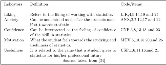
Furthermore, in order to obtain data for their empirical study, they used the ATS scale of [12]. This scale was applied to 298 students. This instrument indicates the existence of five factors: usefulness, anxiety, confidence, liking and motivation. Table 3 described the indicators, definitions and codes/items.

Table 3: Scale factors attitude toward statistics.

Indicators Definition Code/items

Liking Refers to the liking of working with statistics. LIK,4,9,14,19 and 24 Anxiety Can be understood as the fear the students

man-ifest towards statistics

ANX,2,7,12,17 and 22

Confidence Can be interpreted as the feeling of confidence of the skill in statistics.

CNF,3,8,13,18 and 23

Motivation What the student feels towards the studying and usefulness of statistics.

MTV,5,10,15,20,and 25

Usefulness It is related to the,value that a student gives to statistics for his/her professional future.

USF,1,6,11,16,and 21

(19)

With this information and the same data base, we carry out the calculations in order to validate the pertinence to use the exploratory factorial analysis technique (EFA) as mentioned in point 1.1 and 1.2 in this work.

Firstly, we obtained the descriptive statistics and afterwards, we carry out the test of Sphericity with KMO, and goodness of fit indexX2 _df _{with significance}_α_{=0.01, Also, we} obtain the correlation matrix with its determinant, Anti-image Matrices, Component ma-trix and communalities, Component Mama-trixa rotated and communalities, Total Variance Explained and finally sedimentation plot.

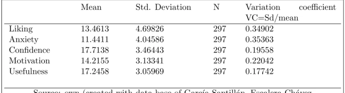
Table 4: Descriptive Statistics

Mean Std. Deviation N Variation coefficient VC=Sd/mean

Liking 13.4613 4.69826 297 0.34902

Anxiety 11.4411 4.04586 297 0.35363

Confidence 17.7138 3.46443 297 0.19558

Motivation 14.2155 3.13341 297 0.22042

Usefulness 17.2458 3.05969 297 0.17742

Source: own (created with data base of Garc´ıa-Santill´an, Escalera-Ch´avez and Venegas-Mart´ınez, 2014)

Table 5: KMO and Bartlett’s Test

Kaiser-Meyer-Olkin Measure of Sampling Adequacy. .630 Bartlett’s Test of Sphericity Approx. Chi-Square 361.034

df 10

Sig. 0.000

(20)

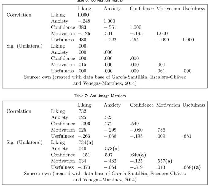
Table 6: Correlation Matrixa

Liking Anxiety Confidence Motivation Usefulness Correlation Liking 1.000

Anxiety −.248 1.000

Confidence .383 −.561 1.000

Motivation −.126 .501 −.195 1.000

Usefulness .480 −.222 .455 −.090 1.000 Sig. (Unilateral) Liking .000

Anxiety .000 .000

Confidence .000 .000 .000

Motivation .015 .000 .000 .000

Usefulness .000 .000 .000 .061 .000 Source: own (created with data base of Garc´ıa-Santill´an, Escalera-Ch´avez

and Venegas-Mart´ınez, 2014)

Table 7: Anti-image Matrices

Liking Anxiety Confidence Motivation Usefulness Correlation Liking .732

Anxiety .025 .523

Confidence −.096 .272 .549

Motivation .025 −.299 −.080 .736

Usefulness −.263 −.038 −.195 .009 .681 Sig. (Unilateral) Liking .734(a)

Anxiety .040 .578(a)

Confidence −.151 .507 .640(a)

Motivation .034 −.482 −.125 .557(a)

Usefulness −.373 −.064 −.319 .013 .668)(a) Source: own (created with data base of Garc´ıa-Santill´an, Escalera-Ch´avez

and Venegas-Mart´ınez, 2014)

At the end, all this procedure allows us to identify the explanation power of the model, i.e., with the component matrix and its communalities, we obtain the eigenvalue and its percentage of total variance.

Now we carry out a measurement of the attitude toward statistics through structural equations, all this, in order to identify if the components of model proposed by Auzmendi [12] will be able to show an alternative model.

2.8. Measurement attitude toward statistics through structural equation (AMOS)

(21)

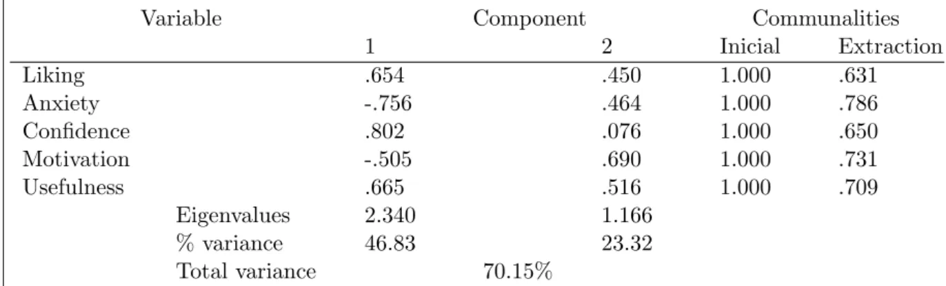
Table 8: Component Matrixa_{and communalities}

Variable Component Communalities

1 2 Inicial Extraction

Liking .654 .450 1.000 .631

Anxiety -.756 .464 1.000 .786

Confidence .802 .076 1.000 .650

Motivation -.505 .690 1.000 .731

Usefulness .665 .516 1.000 .709

Eigenvalues 2.340 1.166

% variance 46.83 23.32

Total variance 70.15%

Extraction Method: Principal Component Analysis. a. 2 components extracted. Source: own (created with data base of Garc´ıa-Santill´an, Escalera-Ch´avez and Venegas-Mart´ınez, 2014)

Table 8.1: Component Matrixarotated and communalities

Variable Component Communalities

1 2 Inicial Extraction

Liking .792 -.067 1.000 .631

Anxiety -.290 .838 1.000 .786

Confidence .669 -.450 1.000 .650

Motivation .047 .854 1.000 .731

Usefulness .842 -.023 1.000 .709

Eigenvalues 1.870 1.639

% variance 37.371 32.776

Total variance 70.145%

Extraction Method: Principal Component Analysis. Rotation Method: Varimax with Kaiser Normalization. a a. Rotation converged in 6 iterations.

2.8.1. Research question

(22)

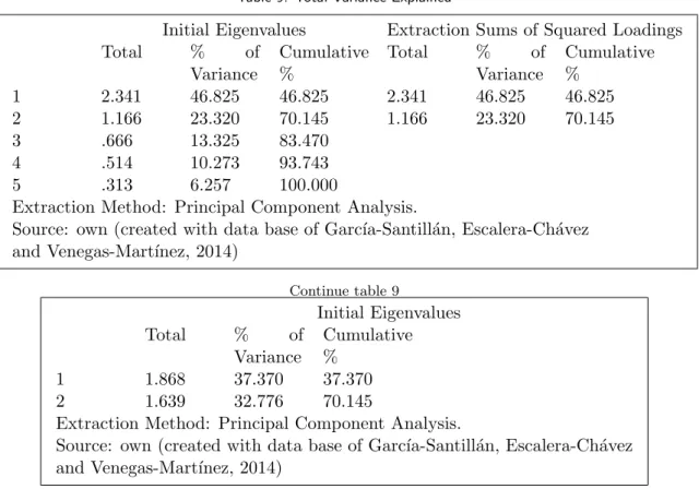
Table 9: Total Variance Explained

Initial Eigenvalues Extraction Sums of Squared Loadings

Total % of

Variance

Cumulative %

Total % of

Variance

Cumulative %

1 2.341 46.825 46.825 2.341 46.825 46.825

2 1.166 23.320 70.145 1.166 23.320 70.145

3 .666 13.325 83.470

4 .514 10.273 93.743

5 .313 6.257 100.000

Extraction Method: Principal Component Analysis.

Continue table 9

Initial Eigenvalues

Total % of

Variance

Cumulative %

1 1.868 37.370 37.370

2 1.639 32.776 70.145

Extraction Method: Principal Component Analysis.

2.8.2. Objectives:

So1. Develop a theoretical model that integrates the factors that explain attitude toward

statistics.

So2. Evaluate the model using the elements of each factor.

So3. Evaluate the adjusted model.

2.8.3. Hypotheses:

H1: There are factors that can help explain the attitude toward statistic in undergraduate Students

(23)

For that, we start from the model developed by Auzmendi [30] which includes latent variables that represent non-observable concepts and their possible measurement through the use of SEM, due to its capacity to include latent variables. Furthermore, this model SEM represents the measurement error in the estimation process [20].

To get objectives SO2 and SO3, we should use the approach of two steps for SEM; measurement of model and structural model. The measurement model followed by an estimate of the structural model is estimated. The measurement model consists of a confirmatory factor analysis (CFA) that assesses the contribution of each variable and its indicators to measure the adequacy of the measurement model.

Several tests of Goodness of Fit (GOF) measures are used in this study; these include the likelihood ratio chi-square (X 2), the ratio ofX 2 to degrees of freedom (X 2 /df), the Goodness of Fit Index (GFI), the Adjusted Goodness of Fit Index (AGFI), the Root Mean Square Error of Approximation (RMSEA) and Tucker-Lewis (TLI) index [20]. The guidelines for acceptable values for these measures are discussed below.

A non-significant X 2 (p>0.05) is considered a good fit for theX 2 the GOF measure; however, this does not necessarily mean a model with significantX 2, to be a poor fit. As a result, a consideration of the ratio of X 2 to degrees of freedom (X 2 /df) is proposed to measure as an additional measure of GOF. A value smaller than 3 is recommended for the ratio (X 2 /df) for accepting the model to be a good fit [10].

The GFI has been developed to overcome the limitations of the sample size dependent

X 2 measures as GOF (Joreskog, et al. 1993). A GFI value higher than 0.9, is recom-mended as a guideline for a good fit. An extension of the GFI is the AGFI, adjusted by the ratio of degrees of freedom for the proposed model to the degrees of freedom for the null model. An AGFI value greater than 0.9 is an indicator of good fit [29].

RMSEA measures the mean discrepancy between the population estimates from the model and the observed sample values. RMSEA<0.1 indicates good model fit [20]. TLI, an incremental fit measure, with a value of 0.9 or more indicates a good fit (Hair, et al. 1998). Except for TLI, all the other measures are absolute GOF measures. The TLI measure compares the proposed model to the null model.

Based on the guidelines for these values, problematic items that caused unacceptable model fit were excluded to develop a more parsimonious model with a limited number of items. The steps to follow are the following:

1. The first step in CFA is the model specification.

2. The second step is an iterative model which consists of the modification of the process to develop a more parsimonious set of items to represent a construct through refinement and retesting.

3. The third step is to estimate the parameters of the specified model.

(24)

item 1 item 6 item 11 item 21 item 2 item 17 item 22 item 4 item 9 item 14 item 19 item 24 item 8 item 13 item 5 item 10 e 1 e 2 e 3 e 4 e 5 e 6 e 7 e 8 e 9 e 10 e 11 e 12 e 13 e 14 e 15 e 16 u A L C M 22 22 22 27 74 70 57 63 68 74 74 69 60 79 68 70 70 66 41 82 35 60 55 70 24 66

Figure 1: Sequence Diagram (source: taken from [17])

Table 10: Weighting of constructs

Usefulness Anxiety Confidence Likeness Motivation Variable

Weighting Significance

Ítem 1 0.793 Ítem 2 0.702 Ítem 8 0.702 Ítem 4 0.711 Ítem 5 0.665

Variable Weighting Significance

´Item 6 0.704 11.610

´Item 17 0.732 10.403

´Item 13 0.69 9.130

Ítem 9 0.599 9.433 Ítem 10 0.534 6.387 Variable Weighting Significance Ítem 11 0.624 10.241 Ítem 22 0.743 10..497 Ítem 14 0.794 12.224 Variable Weighting Significance Ítem 21 0.627 10.301

´Item 19 0.69 10.793 Variable Weighting Significance ´Item 24 0.688 10.764

2.9. Conclusion

At the end of this essay, we could say that the main purpose of this work was achieved. Firstly, the theoretical path was showed. Afterwards the measurements of a set of latent variables associated with the phenomenon under study –the specific case the attitude of students towards statistics– were performed.

(25)

Table 11: Correlation between constructs

Usefulness Anxiety Likeness Motivation Confidence

Usefulness 1 0.380 0.770 -0.509 0.546

Anxiety 1 0.360 -0.699 0.676

Likeness 1 -0.238 0.658

Motivation 1 -0.222

Confidence 1

Table 12: Measures Goodness of Fit: Revised model and null

Chi-square ( X2) 236.851 Comparative Fit Index (CFI)

0.907

Degree of freedom (df) 94 Adjusted Goodness of Fit Index (AGFI)

0.874

Significance level (sig.) 0.000 Root Mean Square Er-ror of Approximation (RMSEA)

0.072

Normed Chi-square (

X2/gl )

2.374 Tucker Lewis Index (TLI)

0.893

Goodness of Fit Index (GFI)

0.913 Normed Fit Index (NFI)

0.869

Auzmendi [12].

Afterwards, the development of section 2.7 called hypothetical assumptions, used the databases of the work of Garc´ıa-Santill´an et al [34] and Escalera-Chavez et al [17]. For performing the EFA software SPSS v.23 was used, and for structural equation modeling (SEM) software AMOS v.23 was used.

In the case of EFA we could observe first, the value of the Bartlett Test of Sphericity with KMO (0.648), Chi square X2 379 674 with df 10, sig. 0.00 < p 0.01, the value of each variable MSA (LIK 0.628; ANX 0.602; CNF 0.731; MTV 0.610 and USF 0.649, are within acceptable values >0.50 as well as values of the correlation matrix, gave support to validate the use of this technique, besides giving enough evidence to reject the null hypothesis in the study of Garc´ıa-Santill´an [34].

(26)

Table 13: Reliability and variance of constructs

Indicators Reliability Extracted means variance

Usefulness 0.783 0.476

Anxiety 0.769 0.526

Likeness 0.657 0.489

Motivation 0.825 0.488

Confidence 0.530 0.363

Table 14: Discriminant validity

Usefulness Anxiety Confidence Likeness Motivation

Usefulness (U) 0.690 0.144 0.592 0.259 0.298

Anxiety (A) 0.726 0.129 0.488 0.456

Confidence (C) 0.602 0.056 0.432

Likeness (L) 0.700 0.049

Motivation (M) 0.700

extracting the proportion of variance represented by their communalities, was performed. Hence, the value of each of the eigenvalues and the percentage of the total variance ex-plained was obtained.

As a result of this calculation two factors were obtained: one composed of three ele-ments (usefulness, confidence and liking) and the other composed of two eleele-ments (anxiety and motivation). Eigenvalues 2.340 and 1.166 (with 46.83% of the variance and 23.32% re-spectively) give an explanation of the total variance of 70.15%. Also in the rotated matrix were obtained two factors: one composed of three elements (usefulness, liking and con-fidence) and the other composed of two elements (anxiety and motivation). Eigenvalues 1.870 and 1.639 (with 37.37% of the variance and 32.77% respectively) give an explanation of the total variance of 70.14%.

(27)

Table 15: Measures of Goodness Fit (Model 2)

Chi-square ( X2) 151.580 Comparative Fit Index (CFI)

0.885

Degree of freedom (df) 88 Adjusted Goodness of Fit Index (AGFI)

0.970

Significance level (sig.) 0.000 Root Mean Square Er-ror of Approximation (RMSEA)

0.049

Normed Chi-square (

X2/gl )

1.722 Tucker Lewis Index (TLI)

0.949

Goodness of Fit Index (GFI)

0.940 Normed Fit Index (NFI)

0.916

Usefulness Anxiety Con dence Likeness Motivation

Indicator 1 6 11 16 21

Indicator 5 10 15 20 25

Figure 2: Sequence Diagram (source: taken from [17])

Regarding goodness of fit of the revised model and null, Table 12 provides the quality measures of absolute fit, as well as, the value of Chi square and the indices GFI, AGFI and RMSR. The values obtained were: X2 (236.851 with df 94) is not significant 0.000 but, GFI 0.913 and AGFI 0.874 showed a satisfactory fit, therefore, they are satisfactory because their values tend to 1 and are > 0.5. Also, RMSEA 0.072 is according to the acceptance parameters.

(28)

Figure 3: Model 2 Factorial structure of Auzmendi (source: taken from [17])

of the variance is not considered for the construct. But, usefulness.476), liking 0.489 and motivation 0.488 are very close to 0.5 which is the recommended value for the average variance extracted (Fornell and Larcker, 1981, cited by [25])

Regarding discriminant validity, the values shown in Table 14 reveal that all are less than 1; hence, none of the items were part of the different factors, shown in the other constructs. Thompson (2004) refers that confirmatory factor analysis type should confirm the theoretical model fit, because it is recommendable to compare the fit indices of several alternative models to select the best. Therefore, Escalera-Ch´avez et al [17] verified the model obtained from exploratory factor analysis, which included paths between latent variables, also, they carried out the model estimation (Figure 2).

In the work of Escalera-Ch´avez et al [17] and after a review of the theoretical criteria in terms of their optimal values, we observed that there are values indicating a model with a poor fit. Hence, it was necessary to make some changes in specifications in order to identify a model that best represents the data. Thus, for the re-specification of the hypothesized model, it was necessary to add estimated parameters for the model, resulting in a model 2 (figure 3).

Finally, comparing the results of model 1 and model 2, we may observe the value of Chi-square (X2) decreased from 236.851 to 151.58 and the value of RMSEA also decreased from 0.072 to 0.049, while the goodness of fit indices GFI and AGFI improved from 0.913 to 0.940 and from 0.874 to 0.970 respectively. In the same way, the incremental fit measures (TLI and NFI) have enriched and exceeded the recommended level of 0.90. Regarding the error covariances, these suggest a redundancy between items 1 and 11, 2 and 12, and 10 and 11 due to overlap.

(29)

v.23 software were used.

Moreover, to perform calculations that allowed us to see the function for each the formulas described in sections: 1, 1.1, 2 and 2.1,the authorization was obtained to utilize the database of the works of of [17, 34], hence, it was possible to develop section 2.7 and 2.8 in this work.

As additional data, just to confirm what Garca Santilln et al [34] and Escalera-Chavez et al [17] demonstrated: the five-factor model (usefulness, motivation, likeness, confidence and anxiety) proposed by Auzmendi [12] has an impact on the student’s attitude towards statistics. Moreover, Escalera-Chavez et al [17] identified that there is an alternative model which best fits the proposed model by Auzmendi (CFI = 0.907) and (CFI = 0.885).

ACKNOWLEDGEMENTS The authors thank the readers of European Journal of Pure and Applied Mathematics, for making our journal successful. Also my gratitude goes to Josefina C. Santana, Ph. D., for her support and suggestion in grammar and style in this paper. To my partners Milka, Escalera-Chvez and Francisco Venegas-Martnez who authorized the use of the database to carry out this essay, my eternal gratitude to them. Also my gratitude goes to Felipe de Jess Pozos Texon for his support in the latex format of this paper.

References

[1] R. M. Dreger & L. R. Aiken. The identification of number anxiety in a college population. Journal of Educational Psychology, (48):344351, 1957.

[2] E. Satake & P. P. Amato. Mathematics anxiety and achievement among Japanese el-ementary school students. Educational and Psychological Measurement, 55:10001007, 1995.

[3] D. Redfield & C. Martray B. Moore, L. Alexander. The mathematics anxiety rating scale abbreviated: A validity study. InPaper presented at the meeting of the American Educational Research Association, New Orleans, 1988.

[4] L. Hu & P. M. Bentler. Cutoff criteria for fit indices in covariance structure analysis: Conventional criteria versus new alternatives. Structural Equation Modeling. 1(6):1– 55, 1999.

[5] L. T. Hu & P. M. Bentler. Evaluating model fit. In R. H. Hoyle (Ed.), Structural Equation Modeling. Concepts, Issues, and Applications. London: Sage, 1995.

[6] P.M. Bentler. Eqs structural equations program manual. BMDP Statistic Software, 1989.

(30)

[8] P.M. Bentler & D.G. Bonett. Significance tests and goodness of fit in the analysis of covariance structures. Psychological Bulletin, 88:588–606, 1980.

[9] R. E. Lushene P. R. Vagg & G. A. Jacobs C. D. Spielberger, R. L. Gorsuch. State-Trait Anxiety Inventory for adults sampler set: Manual, test, scoring key. Mind Garden, California, 1983.

[10] W.W. Chin and P. A. Todd. On the use, usefulness and ease of structural equation modeling in MIS research: A note of caution. MIS quarterly, 19(2):237–247, 1995.

[11] D. W. Straub D. Gefen and M. Boudreau. Structural equation modelling and re-gression: Guidelines for research practice. Communications of the Association for Information Systems (AIS), 7(4), 2000.

[12] E.Auzmendi. Evaluacin de las actitudes hacia la estadstica en alumnos universitarios y factores que las determinan. PhD thesis. PhD thesis, Universidad de Deusto, Bilbao, 1992.

[13] R. M. Suinn & R. Edwards. The measurement of mathematics anxiety. The Mathe-matics Anxiety Rating Scale for AdolescentsMARS-A.Journal of Clinical Psychology, 38:576577, 1982.

[14] A. Garca-Santilln; M. E. Escalera-Chvez and A. Crdova-Rangel. Variables to measure interaction among mathematics and computer through structural equation modeling.

Journal of Applied Mathematics and Bioinformatics, 3(2):51–67, 2012.

[15] A.Garca-Santilln; F. Venegas-Martnez; M. E. Escalera-Chvez and A. Crdova-Rangel. Attitude towards statistics in engineering college: An empirical study in public uni-versity (UPA). Journal of Statistic and Econometric Methods, 1(2):43–60, 2013.

[16] A.Garca-Santilln; M. E. Escalera-Chvez and F. Venegas-Martnez. Principal compo-nents analysis and Factorial analysis to measure latent variables in a quantitative research: A mathematical theoretical approach. Bulletin of Society for Mathematical Service and Standars,, 2(3):3–14, 2013.

[17] M. E. Escalera-Chvez; A. Garca-Santilln and F. Venegas-Martnez. Modeling attitude toward Statistic with structural equation. Eurasia Journal of Mathematics, Science & Technology Education, 10(1):23–31, 2014.

[18] J. B. Rounds & D. D. Hendel. Measurement and dimensionality of mathematics anxiety. Journal of Counseling Psychology, 27:138149, 1980.

[19] E. Levitt & L. Hutton. A psychometric assessment of the Mathematics Anxiety Rating Scale. International Review of Applied Psychology, 33:233242, 1984.

(31)

[21] J. Viehe & S. Segal J. H. Resnick. Is math anxiety a local phenomenon? A study of prevalence and dimensionality. Journal of Counseling Psychology, 29:3947, 1982.

[22] R. Kazelskis. Some dimensions of mathematics anxiety: A factor analysis across instruments. Educational and Psychological Measurement, 58:623633, 1998.

[23] J. L. Ling. A factor analytic study of mathematics anxiety. Unpublished doctoral dissertation. PhD thesis, Virginia Polytechnic Institute and State University, 1982.

[24] A. Wigfield & J. L. Meece. Math anxiety in elementary and secondary school students.

Journal of Educational Psychology, 80:210–216, 1988.

[25] A. Calvo De Mora and F. Criado. Anlisis de la validez del modelo europeo de ex-celencia para la gestin de la calidad en las Instituciones universitarias: un enfoque directivo. Revista Europea de Direccin y Economa de la Empresa, 14(3):41–58, 2005.

[26] B. S. Plake & C. S. Parker. The development and validation of a revised version of the Mathematics Anxiety Rating Scale. Educational and Psychological Measurement, 42:551557, 1982.

[27] E. Nicoletti & P. R. Spinelli R. M. Suinn, C. A. Edie. The MARS, a measure of mathematics anxiety: Psychometric data. Journal of Clinical Psychology, 28:373375, 1972.

[28] R. S. Sandman. The mathematics attitude inventory: Instrument and users manual.

Journal for Research in Mathematics Education, 11:148149, 1980.

[29] A. H. Segars and V. Grover. Re-examining perceived ease of use and usefulness: A confirmatory factor analysis. MIS quarterly, 17(4):517–525, 1993.

[30] E. Fennema & J.A. Sherman. Fennema-Sherman Mathematics Attitude Scale: Instru-ments designed to measure attitudes toward the learning of mathematics by females and males. JAS Catalog of Selected Documents in Psychology,, 31(6), 1976.

[31] C. D. Spielberger. Preliminary professional manual for the test anxiety inventory. Consulting Psychologists Press, Palo Alto, CA, 1980.

[32] V. W. Strawderman.A description of mathematics anxiety using an integrative model. Unpublished doctoral dissertation. PhD thesis, Georgia State University., 1985.

[33] F.C. Richardson & R. M. Suinn. The Mathematics Anxiety Rating Scale: Psycho-metric data. Journal of Counseling Psychology, 19:551554, 1972.

(32)

[35] R. M. Suinn & E. H. Winston. The mathematics anxiety rating scale, a brief version: Psychometric data. Psychological Reports 92, 2003.