METHODS IN RANDOMIZATION BASED ANCOVA FOR NOVEL CROSSOVER DESIGNS AND SENSITIVITY ANALYSIS FOR MISSING DATA
Siying Li
A dissertation submitted to the faculty at the University of North Carolina at Chapel Hill in partial fulfillment of the requirements for the degree of Doctor of Philosophy in the
Department of Biostatistics in the Gillings School of Global Public Health.
Chapel Hill 2017
Approved by: Gary G. Koch Amy H. Herring
Anastasia Ivanova
© 2017 Siying Li
ABSTRACT
Siying Li: Methods in Randomization Based ANCOVA for Novel Crossover Designs and Sensitivity Analysis for Missing Data
(Under the direction of Gary G. Koch)
In clinical trials, statistical inference is preferably conducted with less stringent assumptions. This dissertation proposes a non-parametric method for dichotomous and ordinal missing data, and it proposes a structure for the hypothesis testing and estimation for innovative crossover designs.
When data missing not at random (MNAR) arise from randomized visit, multi-center clinical trials, sensitivity analyses to address possibly informative missing are needed. We propose a closed form point and variance matrix estimation for dichotomized missing data by probabilistically redistributing missing counts, adjusting for a stratification factor and/or baseline covariables. The parameter estimates are computed via weighted least squares asymptotic
regression through randomization based methods. We further extend the methods to sensitivity analyses for ordinal endpoints.
mean and variance estimates under the null hypothesis, which control Type I error well in hypothesis testing. Baseline imbalance is adjusted by randomization-based ANCOVA.
Simulations are performed to study the statistical properties of the proposed methods, which are compared to those of a repeated measures model proposed by Doros et al. (2013).
Point and confidence interval estimation is also addressed by assuming the study population comes from a simple random sample of an almost infinite population. A consistent covariance matrix estimator is constructed and properties of the proposed estimators are studied with simulations, particularly for coverage of confidence intervals. The nominal coverage level is achieved with a t distribution for the approximation to the asymptotic distribution when the sample size is not sufficiently large.
ACKNOWLEDGEMENTS
I want to take the opportunity to express my thanks to Dr. Gary Koch, who supported me both financially and mentally throughout my graduate school years. His role as mentor of life and his advice on both research and life (and Carolina basketball and football), in the office, at breakfast in Bob Evans and Whole Foods, and over the phone whenever I needed, will always be a memorable experience. My gratitude also goes to Dr. Amy Herring, for coaching me on
research projects and serving as my role model as a passionate public health female researcher. Their being my pillar of support and always backing me up has encouraged me through both my good and struggling times. I also want to thank Dr. Preisser and Dr. Ivanova for being coauthors of manuscripts and for the constructive feedbacks they have provided, and Dr. Poole for being on my committee.
I would like to thank my grandparents and parents, who have always set the bar high since I was a kid and believed in my capability in accomplishing goals. I could not express my gratitude enough to my husband, who always support me unconditionally, with great patience along my way. I am also grateful for my fellow students at UNC, SPH, and the biostat
TABLE OF CONTENTS
LIST OF TABLES ... ix
LIST OF FIGURES ... xi
CHAPTER 1 INTRODUCTION ... 1
Handling Random Imbalance of Baseline Covariables ... 1
Handling Missing Data... 4
1.2.1 Missing Data Mechanism ... 5
1.2.2 Approaches for Handling Dropouts by Parametric Model ... 9
1.2.3 Approaches for Handling Dropouts by Imputation ... 11
1.2.4 Sensitivity Analyses ... 14
Crossover Studies ... 15
1.3.1 Traditional Crossover Designs ... 15
1.3.2 Innovative Two-Period Crossover Designs ... 17
Summary ... 23
REFERENCES ... 25
CHAPTER 2: SENSITIVITY ANALYSIS OF FAVORABLE PROPORTION FOR MISSING DICHOTOMOUS DATA IN MULTI-VISIT RANDOMIZED CLINICAL TRIAL ... 28
Introduction ... 28
Methods ... 29
2.2.1 Notation... 30
2.2.2 Data Structure ... 30
2.2.4 Sensitivity Analysis ... 32
2.2.5 Covariance Matrix Estimation ... 34
2.2.6 Treatment Comparison... 36
Example ... 39
Discussion ... 42
REFERENCES ... 43
CHAPTER 3: SENSITIVITY ANALYSIS IN TREATMENT COMPARISON FOR MISSING ORDINAL DATA IN MULTIE-VISIT RANDOMIZED CLINICAL TRIAL ... 44
Introduction ... 44
Methods ... 44
3.2.1 Notation... 44
3.2.2 Data Structure ... 45
3.2.3 Multinomial Probability Estimation ... 46
3.2.4 Sensitivity Analysis ... 46
3.2.5 Treatment Comparison... 49
Example ... 54
REFERENCES ... 57
CHAPTER 4: RANDOMIZATION-BASED ANCOVA FOR HYPOTHESES TESTING IN THE SEQUENTIAL PARALLEL COMPARISON DESIGN (SPCD) ... 58
Introduction ... 58
Methods ... 61
Simulation Study ... 69
4.3.1 Simulation Setup ... 69
4.3.2 Simulation Results ... 71
REFERENCES ... 80
CHAPTER 5: RANDOMIZATION-BASED ANCOVA FOR POINT AND CONFIDENCE INTERVAL ESTIMATION IN SEQUENTIAL PARALLEL COMPARISON DESIGN (SPCD) ... 82
Introduction ... 82
Methods ... 82
Simulation Study ... 87
5.3.1 Simulation Setup ... 87
5.3.2 Simulation Results ... 89
REFERENCES ... 98
CHAPTER 6: RANDOMIZATION-BASED ANCOVA FOR INFERENCE IN TWO-WAY ENRICHMENT DESIGN ... 99
Introduction ... 99
Methods ... 99
6.2.1 Estimates for Treatment Comparisons ... 100
6.2.2 Randomization-Based Covariance Adjusted Estimators ... 102
REFERENCES ... 105
CHAPTER 7: RANDOMIZATION-BASED ANCOVA FOR INFERENCE IN BILATERAL DESIGN ... 106
Introduction ... 106
Methods ... 106
7.2.1 Estimates for Treatment Comparisons ... 107
7.2.2 Randomization-Based Covariance Adjusted Estimators ... 110
LIST OF TABLES
Table 1.1 2×2 Design Parameters ... 16
Table 2.1 Data Structure ... 30
Table 2.2 Data Structure for Missing Counts Redistribution ... 32
Table 2.3 Missing Percentages of Assessment Visits ... 39
Table 2.4 Results of Sensitivity Analyses for Treatment Comparison Estimators ... 41
Table 3.1 Data Structure ... 45
Table 3.2 Data Structure for Missing Counts Redistribution ... 47
Table 3.3 Missing Counts of Assessment Visits ... 54
Table 3.4 Results of Sensitivity Analyses... 56
Table 4.1 Specifications for Assessments of Statistical Power ... 70
Table 4.2 Results from 50, 000 replicate simulations for the test statistics of H0: Δ1 = Δ4 = 0 under Δ1 = Δ2 = Δ3 = Δ4 = 0 ... 73
Table 4.3 Results from 50, 000 simulations for the test statistics of H0: Δ1 = Δ3 = Δ4 = 0 under Δ1 = Δ2 = Δ3 = Δ4 = 0 ... 74
Table 4.4 Results from 50, 000 replicate simulations for the test statistics of H0: Δ1 = Δ3 = Δ3 = Δ4 = 0 under Δ1 = Δ2 = Δ3 = Δ4 = 0 ... 75
Table 4.5 Results from 50,000 replicate simulations for power of test statistics under the alternative specified in Table 4.1 ... 76
Table 4.6 Mean and Standard Deviation of Outcome... 77
Table 4.7 Estimates of Δ1 to Δ4 ... 78
Table 4.8 Estimates of Weighted Statistics... 79
Table 5.1 Specifications for Assessments of Statistical Power ... 88
Table 5.2 Results from 50, 000 replicate simulations for the test statistics of H0: Δ1 = Δ4 = 0 under Δ1 = Δ2 = Δ3 = Δ4 = 0 ... 91
Table 5.4 Results from 50, 000 replicate simulations for the test statistics of
H0: Δ1 = Δ3 = Δ3 = Δ4 = 0 under Δ1 = Δ2 = Δ3 = Δ4 = 0 ... 93
Table 5.5 Results from 50,000 replicate simulations for the coverage of confidence intervals and power of test statistics under the alternative specified in Table 5.1 ... 94
Table 5.6 Mean and Standard Deviation of Outcome... 95
Table 5.7 Estimates of ∆1 to ∆4 ... 96
LIST OF FIGURES
Figure 1.1 Randomized Withdrawal Design ... 19
Figure 1.2 Placebo Lead-In Design ... 19
Figure 1.3 P:T, T:P, and T:T Sequence Design ... 20
Figure 1.4 Randomized Delayed-Start Design ... 21
Figure 1.5 SPCD Design ... 22
CHAPTER 1 INTRODUCTION
In clinical trials, statistical inference is preferably conducted with less model
assumptions. This dissertation proposes a nonparametric method to handle dichotomous and ordinal missing data, and proposes a structure for hypothesis testing and estimation in innovative crossover designs.
Handling Random Imbalance of Baseline Covariables
In the statistical analysis plan of a clinical trial, the statistical methods to determine if there is a significant treatment effect need to be stated in an a priori way before the clinical trials are actually carried out. Oftentimes, assumptions have to be made for certain statistical models to be valid, and they are difficult to test before data analysis. Therefore, methods requiring fewer assumptions are more desirable than those complicated ones, especially in the regulatory setting.
This consideration led to the development of nonparametric randomization based analysis of covariance (ANCOVA). In randomized clinical trials, the covariable imbalances (if any) between treatment and control groups are due to random chance, since the treatment assignment is random.
Let 𝑦𝑔𝑖 be the outcome of subject 𝑖 in group 𝑔, and let 𝒙𝑔𝑖 = (𝑥𝑔𝑖1, … , 𝑥𝑔𝑖𝑚)′ be the pre-specified vector of m covariables, and let 𝒇𝑔𝑖 be the response-covariable (m+1) dimensional vector (𝑦𝑔𝑖, 𝒙𝑔𝑖′ )′. Then the sample mean of the outcome and covariables of treatment 𝑔 is 𝑦̅𝑔 =
1
𝑛𝑔∑ 𝑦𝑔𝑖
𝑛𝑔
𝑖=1 and 𝒙̅𝑔 = 1
𝑛𝑔∑ 𝒙𝑔𝑖
𝑛𝑔
𝑖=1 . And 𝒇̅𝑔 = 1
𝑛𝑔∑ 𝒇𝑔𝑖 = (𝑦̅𝑔,
𝑛𝑔
𝑖=1 𝒙̅𝑔′)′ is the sample mean of the
response-covariables of subjects in group 𝑔 and 𝒇̅ =1
𝑛∑ ∑ 𝒇𝑔𝑖 𝑛𝑔
𝑖=1 2
𝑔=1 is the sample mean of all subjects in the trial. Let 𝒅 = (𝑑𝑦, 𝒅𝒙′)′ be the vector of differences in means, where 𝑑
𝑦 = (𝑦̅1−
𝑦̅2) and 𝑑𝑥= (𝒙̅1− 𝒙̅2).
There are two ways to estimate the variance of the difference 𝒅. One is through the randomization distribution of 𝒅 for the finite population selected for the clinical trial assuming the strong null hypothesis 𝐻0: 𝑦1𝑖 = 𝑦2𝑖 = 𝑦∗𝑖 that each patient would have the same outcome regardless of the assigned treatment. Under this null hypothesis, the covariance matrix for the difference 𝒅 is expressed as
𝑽𝟎 = 𝑛
𝑛1𝑛2(𝑛 − 1)∑ ∑[𝒇𝑔𝑖− 𝒇̅][𝒇𝑔𝑖− 𝒇̅] ′ 𝑛𝑔
𝑖=1 2
𝑔=1
(1.1).
Since 𝑽𝟎 is the covariance matrix for the randomization distribution of 𝒅, permuting all possible randomized assignments to the two treatments for the patients in the clinical trial, it is a matrix of known constant values (rather than random variables), with a conditional nature that the response of this finite population is known.
𝑽𝑺 = ∑ 1 𝑛𝑖(𝑛𝑖 − 1)
∑[𝒇𝑔𝑖− 𝒇̅𝑔][𝒇𝑔𝑖− 𝒇̅𝑔]′ 𝑛𝑔
𝑖=1
(1.2). 2
𝑔=1
In this case, the covariance matrix 𝑽𝑺 is a random matrix instead of a constant matrix, in a sense that the randomness comes from the variability of the simple random sample of patients and the random assignment of treatment groups, regardless of 𝐻0.
Applying the non-parametric analysis of covariance to 𝒅, it has the form of a linear regression as below,
𝒅 = [𝑑𝑦 𝒅𝒙
] ≜ 𝒁𝑏 = [ 𝟎1
𝑝] 𝑏 (1.3)
where ≜ denotes “is estimated by”, 𝟎𝑝 denotes a 𝑝 dimensional vector, 𝒁 = [1 𝟎𝑝′]′, and 𝑏 is the adjusted mean difference for the response, i.e., the adjusted version of 𝑑𝑦.
Applying WLS, determination of 𝑏 can be obtained by,
𝑏 = (𝒁′𝑽−𝟏𝒁)−𝟏𝒁′𝑽−𝟏𝒇 = 𝑑𝑦− 𝑽𝒚𝒙′ 𝑽𝒙𝒙−𝟏𝒅𝒙 (1.4)
where 𝑽 = [𝑽𝒚𝒚 𝑽𝒚𝒙 ′
𝑽𝒚𝒙 𝑽𝒙𝒙] and V can be either 𝑽0 or 𝑽𝑆 defined above. An estimator for the covariance of 𝑏 is expressed as,
𝑉𝑏 = (𝒁′𝑽−1𝒁)−1 = 𝑉
𝑦𝑦− 𝑽𝒚𝒙′ 𝑽𝒙𝒙−1𝑽𝒚𝒙 (1.5)
When 𝑽𝟎 is used in place of 𝑽, 𝑽𝒃 is an exact variance of the randomization distribution of the adjusted treatment difference b; and when 𝑽𝑆 is used, 𝑉𝑏 is a random matrix and a
consistent estimator of the covariance matrix of b.
is more powerful than that based on 𝑑𝑦, and the confidence interval of 𝑏 is narrower than that of 𝑑𝑦. The variance reduction of 𝑏 relative to 𝑑𝑦 is based on the correlation between the response and the covariable, and the stronger this correlation, the more variance reduction produced (Koch et al., 1998).
The nonparametric ANCOVA can be extended to multivariate response variables, and other types of data including dichotomized, ordinal, and time to event data (Tangen and Koch, 1999).
Handling Missing Data
In public health studies, repeated measurements of the same subject over time are useful in a number of different contexts, including, but not limited to, reliable estimation by several measurements close in time, testing for a change over time in an experimental study, or comparisons for a difference between treatment groups over time.
In a clinical trial, missing data were planned to be collected but are not present in the database. No matter how well designed and conducted a trial is, some missing data is almost always unavoidable. The consequences of missing data can be wide-ranging in that they might lead to a perceived or real reduction in trial quality and validity, and a reduction in the statistical power of the study.
The validity of many statistical models that can handle missing data relies heavily on the assumptions for the missing data. For example, generalized estimating equations (GEE) must be carried out along with the missing completely at random (MCAR) assumption and the mixed models for repeated measures with a missing at random (MAR) assumption. These assumptions might not be realistic in real life, and possibly not even verifiable.
With the withdrawal reasons, assumptions of missingness could be checked; or when the assumptions could not be verified, sensitivity analyses could be performed under different scenarios to test against the robustness of a study result.
Besides the assumptions of the missingness, the handling of missing data is complicated by the form of the study outcome, for example, non-normality of data, such as dichotomous data, ordinal data, or skewed continuous data.
1.2.1 Missing Data Mechanism
We now review the mechanisms that lead to missing data, and in particular the question of whether the variables that are missing are related to the underlying values of variables that are observed or not observed in the dataset. It is crucial to understand the missing data mechanism before any analyses are carried out since the properties of missing data methods rely heavily on the nature of the dependencies in these mechanisms.
Notation
In the context of a longitudinal trial, we assume that measurements are obtained at J visits at times 𝑗 = 1, ⋯ , 𝐽 for independent subjects 𝑖, 𝑖 = 1, ⋯ , 𝑛.
Let 𝒀 = (𝑦𝑖𝑗) denote an (𝑛 × 𝐽) rectangular data matrix of the measurements without missing values, with the 𝑖-th row 𝒚𝑖 = (𝑦𝑖1, ⋯ , 𝑦𝑖𝐽) being the complete data vector of outcomes for subject 𝑖.
Additionally, let 𝑿𝑖 be the design matrix of covariates for subject 𝑖.
Let 𝒓𝑖 = (𝑟𝑖1, ⋯ , 𝑟𝑖𝐽) be the missing data indicator vector. Specifically, let 𝑟𝑖𝑗=1 if 𝑦𝑖𝑗 is observed and 𝑟𝑖𝑗=0 otherwise.
Given the missing data indicator 𝒓𝑖, we can partition 𝒚𝑖 into (𝒚𝑖𝑂, 𝒚𝑖𝑀), with 𝒚𝑖𝑂 being the observed measurements in 𝒚𝑖 and 𝒚𝑖𝑀 being the missing measurements.
The joint distribution of the data and the missing indicator can be formulated as follows and factored into two parts:
𝑓(𝒚𝑖𝑂, 𝒚𝑖𝑀, 𝒓𝑖|𝑿𝑖, 𝜽, 𝝍) = 𝑓(𝒚𝑖𝑂, 𝒚𝑖𝑀|𝑿𝑖, 𝜽)𝑓(𝒓𝑖|𝒚𝑖𝑂, 𝒚𝑖𝑀, 𝑿𝑖, 𝝍) (1.6)
where 𝜽 denotes the parameter vectors for the data and 𝝍 denote the parameter vectors for the missing data mechanism. The first factor on the right-side is the marginal density of the measurements, and the second factor is the conditional density of the missingness on the measurements.
Missing Completely at Random (MCAR)
𝑓(𝒓𝑖|𝒚𝑖𝑂, 𝒚𝑖𝑀, 𝑿𝑖, 𝝍) = 𝑓(𝒓𝑖|𝝍) (1.7) Note that this assumption doesn’t mean that the missingness itself is random, but rather that this distribution does not depend on the data values.
Therefore, the joint distribution simplifies to
𝑓(𝒚𝑖𝑂, 𝒚𝑖𝑀, 𝒓𝑖|𝑿𝑖, 𝜽, 𝝍) = 𝑓(𝒚𝑖𝑂, 𝒚𝑖𝑀|𝑿𝑖, 𝜽)𝑓(𝒓𝑖|𝝍) (1.8) which indicates the measurement and the missingness are independent.
The missing data 𝒚𝑖𝑀 can be now integrated out from the joint distribution, and so the joint distribution of the observed measurement and the missing indicator becomes
𝑓(𝒚𝑖𝑂, 𝒓𝑖|𝑿𝑖, 𝜽, 𝝍) = 𝑓(𝒚𝑖𝑂|𝑿𝑖, 𝜽)𝑓(𝒓𝑖|𝝍) (1.9)
And thus estimation of 𝜽 can be solely based on the observed information 𝒚𝑖𝑂 and does not depend on the nuisance parameter 𝝍.
Missing at Random (MAR)
An assumption less restrictive than MCAR is that missingness depends only on the components that are observed, i.e., 𝒚𝑖𝑂, and not on the components that are missing, i.e., 𝒚𝑖𝑀.
Under MAR, conditional on the observed data, the missingness is independent of the missing measurements, which is,
𝑓(𝒓𝑖|𝒚𝑖𝑂, 𝒚𝑖𝑀, 𝑿𝑖, 𝝍) = 𝑓(𝒓𝑖|𝒚𝑖𝑂, 𝑿𝑖, 𝝍) (1.10)
Therefore, the full data density becomes
𝑓(𝒚𝑖𝑂, 𝒚𝑖𝑀, 𝒓𝑖|𝑿𝑖, 𝜽, 𝝍) = 𝑓(𝒚𝑖𝑂, 𝒚𝑖𝑀|𝑿𝑖, 𝜽)𝑓(𝒓𝑖|𝒚𝑖𝑂, 𝑿𝑖, 𝝍) (1.11)
𝑓(𝒚𝑖𝑂, 𝒓𝑖|𝑿𝑖, 𝜽, 𝝍) = 𝑓(𝒚𝑖𝑂|𝑿𝑖, 𝜽)𝑓(𝒓𝑖|𝒚𝑖𝑂, 𝑿𝑖, 𝝍) (1.12)
With MAR assumption, the model 𝑓(𝒓𝑖|𝒚𝑖𝑂, 𝑿𝑖, 𝝍) does not need to be specified to obtain valid likelihood based inferences, and only the model 𝑓(𝒚𝑖𝑂, 𝒚𝑖𝑀|𝑿𝑖, 𝜽) is needed.
MCAR and MAR are often referred to as ignorable missing. The ignorability refers to the fact that once 𝑓(𝒓𝑖|𝒚𝑖, 𝑿𝑖) not depending on 𝒚𝑖𝑀 can be established, 𝑓(𝒓𝑖|𝒚𝑖, 𝑿𝑖) can be ignored and a valid likelihood based inference can be obtained given that we model 𝑓(𝒚𝑖𝑂, 𝒚𝑖𝑀|𝑿𝑖, 𝜽) correctly.
Not Missing at Random (NMAR)
If the measurements are NMAR, which means 𝒓𝑖 depends on 𝒚𝑖𝑀, the joint distribution can no longer have 𝒚𝑖𝑀 integrated out. No simplification of the joint distribution is possible.
Under the MNAR assumption, the probability of an observation being missing depends on the underlying missing value, and the joint distribution has to be written as in (1.13),
𝑓(𝒚𝒊𝑶, 𝒓𝒊|𝑿𝒊, 𝜽, 𝝍) = ∫ 𝑓(𝒚𝒊𝑶, 𝒚𝒊𝑴|𝑿𝒊, 𝜽)𝑓(𝒓𝒊|𝒚𝒊𝑶, 𝒚𝒊𝑴, 𝑿𝒊, 𝝍)𝑑𝒚𝒊𝑴 (1.13)
and inferences could only be made by making further assumptions (Molenberghs and Kenward, 2007).
Monotone versus Non-Monotone Missingness
In the clinical trials setting, monotone missingness happens when a study subject withdraws from the trial prematurely and doesn’t come back to the study, which is commonly referred to as dropout or loss to follow up in longitudinal studies; while non-monotone missing is the case when a subject misses one or more intermediate visits but does come back to provide subsequent measurements (O’Kelly and Ratitch, 2014). A dataset is considered as monotone missing only when all the subjects in the study have a monotone pattern, but it is considered as non-monotone missing if there is intermediate missingness in at least one subject.
1.2.2 Approaches for Handling Dropouts by Parametric Model Complete Case Analysis
One approach to handling missing data is to have analyses that exclude all data from any subject who drops out. This method is referred to as a complete-case analysis, which is
performed by excluding any subjects that missed any intended measurement. It is emphasized that this method is very problematic and is rarely an acceptable approach in most occasions (Fitzmaurice, Laird and Ware, 2012). It will yield unbiased estimates of the mean response trends only when the dropout can be assumed as MCAR. When dropout is MCAR, the study completers are a random subsample of the original sample from the population. However, even in occasions where the MCAR assumptions might hold, a complete-case analysis is not an appealing one since it leads to reduction in the number of subjects and hence results in reduction in statistical power.
Generalizing Estimating Equations (GEE)
GEE is a semiparametric method that models a known function of the marginal
of estimating equations and the use of a non-linear link function for the marginal model of the correlated response can facilitate the analyses of continuous or discrete responses.
The correlation of the clustered dependent variable can be specified via a working
correlation matrix and the consistency of parameter estimates do not rely on correct specification of the correlation. The dependent variable doesn’t need to have the same number of elements across clusters and thus in the longitudinal data context, missing data is allowed. However, if the data is MAR, as GEE methods only require a model for the mean response but do not specify the multivariate joint distribution for the response vector, the standard GEE methods do not provide valid estimates of the regression parameters (Fitzmaurice et al., 2012).
An adaption of GEE methods for the MAR assumption is to model the missingness 𝑓(𝒓𝑖|𝒚𝑖, 𝑿𝑖) and weighting the analysis by including it in the estimating equations accordingly
(Robins, Rotnitzky and Zhao, 1995).
Mixed Model for Repeated Measures (MMRM)
1.2.3 Approaches for Handling Dropouts by Imputation Ad-hoc Single Imputation
Imputation replaces the missing values with plausible ones. There are many approaches to do single imputation. The missing values could be filled in from an individual imputation, where these values are coming from the same individual with the actual missing values, or from a group imputation, in which information from the entire sample or a portion of the sample is used to fill in for the missing value of an individual (Fitzmaurice et al., 2012).
Two of the most commonly used individual imputations are, baseline observation carried forward (BOCF) and last observation carried forward (LOCF), where either the baseline value or the last observed value is substituted for the missing values of the study subject. For example, in the LOCF case, if an individual was supposed to have five measurements but only the first three measurements were observed, the last two missing measurements would be filled in with the third value as it was the last observed value before the loss to follow up. The assumption of BOCF or LOCF is conservative in estimating the missing outcome if a subject does benefit from the trial. The imputation using BOCF or LOCF would underestimate the variability of the estimation and result in smaller standard errors estimate. Other single imputation includes the individual mean substitution, the group mean substitution, the individual worst case substitution, or the interpolation of last and next observed values if the missingness is not monotonic.
Multiple Imputation (MI)
SAS, R, and Stata have included procedures or packages to deal with it, which reduces the computational burden and complexity. Multiple imputation is a more flexible and powerful tool to handle incomplete data than the other parametric methods such as GEE and MMRM, in that it has both an imputation model and an analysis model and these two don’t have to be the same, and it is more acceptable in most settings than the single imputation.
Multiple imputation adopts a three-step approach to fill in the incomplete data and analyze the resulting data structure. First, an imputation model is assumed for the missing outcomes, and plausible values for missing observations are imputed with a draw from the imputation model, usually as a posterior distribution of the missing values conditioning on the imputation model covariates and any previous visits is assumed. This process is repeated to reflect uncertainty about the missing values, resulting in the creation of a number of complete datasets. The number of needed imputations depends on the fraction of missing data, and usually a number of K>5 would be sufficient for most applications to obtain acceptable properties (that is, correct confidence interval coverage) (Carpenter and Kenward, 2012). Second, each of these K complete datasets is analyzed with an analysis model, which need not be the same as the imputation model. Finally, the results are combined for overall inference using Rubin’s combination rule (Rubin, 1987).
Rubin’s combination rule is as follows. Assume the parameter of interest of the complete data analysis is 𝜃 and denote 𝜃̂𝑘 and 𝑉̂𝑘 as the point estimate and variance estimate of 𝜃 from the k-th imputed dataset, 𝑘 = 1, … , 𝐾. Then the MI estimate of 𝜃 can be expressed as the average of the estimates from the 𝐾 complete datasets,
𝜃̂𝑀𝐼 = 1 𝐾∑ 𝜃̂𝑘
𝐾
𝑘=1
The measure of precision for 𝜃̂𝑀𝐼 consists of two parts, the between imputation variance and the within imputation variance. Define
𝑊̂ = 1 𝐾∑ 𝑉̂𝑘
𝐾
𝑘=1
(1.15)
to be the average within imputation variance, and
𝐵̂ = 1
𝐾∑(𝜃̂𝑘− 𝜃̂𝑀𝐼) 2 𝐾
𝑘=1
(1.16)
to be the between imputation variance. Then an estimate of the variance of 𝜃̂𝑀𝐼 is given by
𝑉̂𝑀𝐼 = 𝑊̂ + (1 + 1
𝐾) 𝐵̂ (1.17)
treated as continuous in this partial imputation step. However, in the clinical trial setting, when multiple clinical centers need to be adjusted for, and when the number of centers is large (>10), the center variable might have to be removed from the multivariate normal model for the partial imputation. This assumption could be reasonable if the non-monotone missingness doesn’t vary by center, otherwise the imputed values would not have taken into account the variability introduced by study center.
1.2.4 Sensitivity Analyses
Sensitivity analysis in missing data situations is usually carried out through stressing the assumption of MAR. It is important to examine the sensitivity of statistical inferences when departures from the MAR assumption are in question, because this assumption cannot be verified using the data (O’Kelly and Ratitch, 2014). In this regard, the primary purpose of a sensitivity analysis in a clinical trial is to seek to answer the question that if plausible unfavorable outcomes happen to the withdrawal in the experimental treatment, does the significant results drawn from the primary analysis remain credible or not?
Research Council Panel, 2010). The tipping point in this range of assumptions is the value that overturns the conclusion from being favorable to the experimental treatment, to being not different from the reference group. In terms of hypothesis testing of a treatment effect, the tipping point is the value at which the p value of the test changes from significant to non-significant.
Crossover Studies
Crossover studies are experimental designs for which each subject is randomly assigned to receive a sequence of treatments during consecutive periods for some response variables. There are many possible designs of crossover studies, depending on the number of treatments to compare, the number of periods of each treatment, and the aim of the trials (Jones and Kenward, 2014).
1.3.1 Traditional Crossover Designs
One of the most well-known crossover designs is the one with two sequence groups for two treatments in two periods. This is also the simplest crossover design, which is known as the 2×2 design, or the two-period two-treatment design. The main advantage of the crossover study is that treatments are compared within subjects, where every subject provides two periods of different treatments and thus removal of the subject effect is enabled by direct comparison within subject (Jones and Kenward, 2014).
ambulatory patients with osteoarthritis of the hip or knee and achieved a low dropout rate. Of the 227 enrolled patients, 218 (96.0%) patients completed the first treatment period and 181 (79.7%) completed both treatment periods.
However, the feature of repeated measurements in crossover designs brings
disadvantages along with its advantages; for example, the possibility that the effect of an earlier period would be carried into the later period, and the potential risk of more dropouts due to longer study duration compared to a single period trial.
Statistical Methods for 2×2 Design
Tudor and Koch (1994) review nonparametric methods for analyzing the traditional crossover studies comparing two treatments with small sample sizes and the parametric counterparts when sample sizes are sufficiently large. The methods apply to various types of outcome including continuous, dichotomous, ordinal, and censored time-to-event response.
In particular, for a 2x2 crossover design with a univariate continuous outcome, the structure for the inference is as shown in Table 1.1.
Table 1.1 2×2 Design Parameters
Group Period 1 Period 2
AB 𝜇 + 𝜋1+ 𝜏𝐴 𝜇 + 𝜋2 + 𝜏𝐵+ 𝜆𝐴 BA 𝜇 + 𝜋1+ 𝜏𝐵 𝜇 + 𝜋2 + 𝜏𝐴 + 𝜆𝐵
𝜏𝐴 and 𝜏𝐵 are direct treatment effects of treatment A and treatment B, and 𝜋1 and 𝜋2 are period effects of periods 1 and 2, and 𝜆𝐴 and 𝜆𝐵 are carryover effects of treatment A and
treatment B respectively.
data from both periods in a few steps. In the first step, one would test 𝐻0, where
𝐻0: 2(𝜏𝐵− 𝜏𝐴) − (𝜆𝐵− 𝜆𝐴) = 0. If the 𝐻0 is contradicted, one moves on to test the equality of carryover effects 𝐻0𝜆: 𝜆𝐴 = 𝜆𝐵; and if this similarity is not contradicted, one could have
confidence that the contradiction of 𝐻0 is mainly due to the difference in treatment effects 𝜏𝐴 and 𝜏𝐵 and the equivalence of testing 𝐻0 and 𝐻0𝜏; or if this equality of carryover effects 𝐻0𝜆 is contradicted, meaning there are different carryover effects by the two treatments, which may partly account for the contradiction of 𝐻0, one would have to move on to compare the difference between treatments only using data from Period 1, which does not depend on the carryover effects.
The above tests in each step could be replaced by the asymptotic tests with approximate distributions when the sample size is sufficiently large (sample size per sequence ≥15).
A more comprehensive review of analyses in the traditional 2x2 design and other higher order designs is provided in Jones and Kenward (2014).
1.3.2 Innovative Two-Period Crossover Designs
Innovative crossover designs can have multiple designs embedded within them, which are also in the general class of re-randomization designs. Instead of re-randomization at the beginning of the second period, randomization before the trial could be performed to get the randomized sequences. Without loss of generality, this literature review limits the scope of the discussion to the design with fixed randomization sequences at the initiation of the study without re-randomization later.
populations. Other advances of crossover designs with this structure could be made use of with other added design features, such as enrichment.
Enriched Two-Sequence Design
Common crossover designs that use two of four sequence groups are the T:P, and P:T design (the 2×2 design), the T:P and T:T design, and the P:P and P:T design. The latter two-sequence designs are usually used with enrichment features.
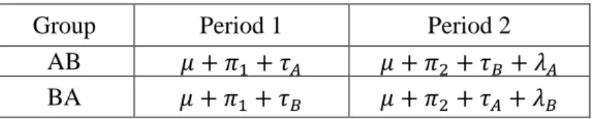
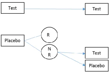
The randomized withdrawal design, with the T:P and T:T sequence groups, makes use of only the patients who respond to the drug in the first period for continuation to the second period. This design is helpful when there is heterogeneity in the patient population itself to respond to a treatment. For example, Temple (1994) discusses situations where the gold standard randomized, double-blind, placebo-controlled study design with continuous treatment might not be able to provide an optimal study when certain diseases are treated, such as irritable bowel syndrome (IBS), a gastrointestinal disorder, which he suggested might be due to IBS being a “common response to a diverse group of abnormality”. The FDA has proposed to conduct clinical trials to include only IBS patients identified by their clinicians as responders to the study treatment (Dunger-Baldauf, Racine, and Koch 2006).
second period to receive either experimental treatment or placebo, the treatment effect is maximized since patients who do not respond to the first period are not expected to become placebo-responders in the second period (Fava et al., 2003).
Figure 1.1 Randomized Withdrawal Design
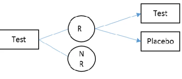
Figure 1.2 Placebo Lead-In Design Three-Sequence Design
Designs with three or more sequence groups could provide additional benefits to the two-sequence designs mentioned above.
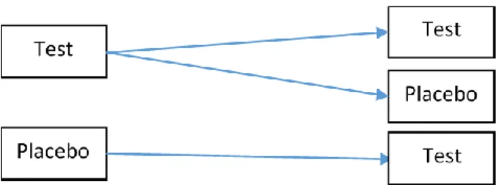
Figure 1.3 P:T, T:P, and T:T Sequence Design
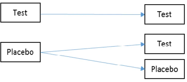
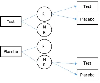
Another design with attractive features also has three sequence groups as P:P, P:T, and T:T, and it is commonly known as the randomized delayed-start design . In this design, patients are initially randomized to placebo or test drug in the first period, and patients who are in the placebo group in the first period would receive either placebo or test drug in the second period, while patients who receive test drug in the first period remain on the same treatment. This design is suitable to evaluate treatments for disease with long term progression to distinguish the
Figure 1.4 Randomized Delayed-Start Design
These two three-sequence designs both have an advantage over the two-sequence
randomized withdrawal design in that there is a higher chance in receiving the better treatment in the second period, which might provide a favorable impact on the patient retention and reduce non-compliance with the protocol, at least at the end of the first period (Dunger-Baldauf, 2007). Enriched Multiple-Sequence Design
Another study design that has the same sequence groups as the randomized delayed-start design is the sequential parallel comparison design (SPCD). SPCD design was proposed by Fava et al. (2013), and it is different from the delayed-start design in that only the placebo
Figure 1.5 SPCD Design
The original paper of Fava et al. (2003) focused on the study outcome as dichotomized data. Other methods have been proposed for the analyses of binary outcomes in the context of SPCD designs by Huang and Tamura (2010), Ivanova, Qaqish and Schoenfeld (2011), and Huang, Tamura, and Boos (2011).
Recent uses of the SPCD design have been extended to continuous or ordinal outcome as it arises more naturally than the dichotomizing of a continuous measurement. Huang and Tamura (2010) considered seemingly unrelated regression (SUR) to account for the correlation between subjects in the two periods of the trial. Chen et al (2011) proposed an ordinary least squares approach and Doros et al. (2013) proposed a repeated measures model that includes all possible outcome data collected in the trial.
The two-way enrichment design (TED), introduced by Ivanova and Tamura (2011), has all four sequence groups, P:P, P:T, T:P, and T:T, but in the second period, only the non-responders to the placebo in the first period of the P:P and P:T sequences, and the responders to the active
(through the randomized withdrawal design) for a disease with a high placebo response rate. For example, for generalized anxiety disorder (GAD), which is a central nerve system disease with a high placebo response rate, and a chronic disease for which worsening would quickly occur after discontinuation from an active treatment, a trial to evaluate an active treatment versus placebo would benefit from the TED design.
Figure 1.6 TED Design Bilateral Design
Besides the studies mentioned above, the four sequence group design could also be applied to two sides of the same subject, instead of two periods. For example, Kawaguchi and Koch (2009) studied the two eyes of the same patients with four sequence group, with the treatments assigned to the two eyes instead of the two periods respectively.
Summary
REFERENCES
Chen, Y.-F., Yang, Y., Hung, H.M.J. and Wang, S.-J. (2011) Evaluation of performance of some enrichment designs dealing with high placebo response in psychiatric clinical trials.
Contemporary Clinical Trials, 32, 592–604.
Doros, G., Pencina, M., Rybin, D., Meisner, A. and Fava, M. (2013) A repeated measures model for analysis of continuous outcomes in sequential parallel comparison design studies.
Statistics in Medicine, 32, 2767–2789.
Dunger-Baldauf, C. (2007) Designs with Randomization Following Initial Study Treatment.
Wiley Encyclopedia of Clinical Trials p. John Wiley & Sons, Inc.
Dunger-Baldauf, C., Racine, A. and Koch, G.G. (2006) Re-treatment studies. Drug Information Journal, 40.
Fava, M., Evins, A.E., Dorer, D.J. and Schoenfeld, D.A. (2003) The problem of the placebo response in clinical trials for psychiatric disorders: culprits, possible remedies, and a novel study design approach. Psychotherapy and Psychosomatics, 72, 115–127. Fitzmaurice, G.M., Laird, N.M. and Ware, J.H. (2012) Applied Longitudinal Analysis. John
Wiley & Sons.
Huang, X. and Tamura, R.N. (2010) Comparison of Test Statistics for the Sequential Parallel Design. Statistics in Biopharmaceutical Research, 2, 42–50.
Ivanova, A., Qaqish, B. and Schoenfeld, D.A. (2011) Optimality, sample size, and power calculations for the sequential parallel comparison design. Statistics in Medicine, 30, 2793–2803.
Jones, B. and Kenward, M. (2014) Design and Analysis of Cross-Over Trials, Third Edition. URL https://www.crcpress.com/Design-and-Analysis-of-Cross-Over-Trials-Third-Edition/Jones-Kenward/p/book/9781439861424 [accessed 16 July 2016]
Kawaguchi, A., Koch, G.G. and Ramaswamy, R. (2009) Applications of extensions of bivariate rank sum statistics to the crossover design to compare two treatments through four sequence groups. Biometrics, 65, 979–988.
Kenward, M. (2012) Multiple Imputation and Its Application. John Wiley & Sons.
Khan, A., Kolts, R.L., Rapaport, M.H., Krishnan, K.R.R., Brodhead, A.E. and Browns, W.A. (2005) Magnitude of placebo response and drug-placebo differences across psychiatric disorders. Psychological Medicine, 35, 743–749.
LaVange, L.M., Durham, T.A. and Koch, G.G. (2005) Randomization-based nonparametric methods for the analysis of multicentre trials. Statistical Methods in Medical Research, 14, 281–301.
Lehmacher, W., Wassmer, G. and Reitmeir, P. (1991) Procedures for two-sample comparisons with multiple endpoints controlling the experimentwise error rate. Biometrics, 47, 511– 521.
Liang, K.-Y. and Zeger, S.L. (1986) Longitudinal data analysis using generalized linear models.
Biometrika, 73, 13–22.
Little, R.J.A. and Rubin, D.B. (2014) Statistical Analysis with Missing Data. John Wiley & Sons. Molenberghs, G. and Kenward, M. (2007) Missing Data in Clinical Studies. John Wiley & Sons. National Research Council Panel. (2010) The Prevention and Treatment of Missing Data in
Clinical Trials. National Academies Press (US), Washington (DC).
O’Kelly, M. and Ratitch, B. (2014) Clinical Trials with Missing Data: A Guide for Practitioners. John Wiley & Sons.
Parkinson’s Disease Edition: Early Diagnosis and Comprehensive Management Table of Contents - Clinical Trial Design in Parkinson’s Disease. URL
http://lmt.projectsinknowledge.com/Activity/index.cfm?showfile=b&jn=2094&sj=2094.0 2&sc=2094.02.3 [accessed 10 August 2016]
Pincus, T., Koch, G.G., Lei, H., Mangal, B., Sokka, T., Moskowitz, R., et al. (2004) Patient Preference for Placebo, Acetaminophen (paracetamol) or Celecoxib Efficacy Studies (PACES): two randomised, double blind, placebo controlled, crossover clinical trials in patients with knee or hip osteoarthritis. Annals of the Rheumatic Diseases, 63, 931–939. Robins, J.M., Rotnitzky, A. and Zhao, L.P. (1995) Analysis of Semiparametric Regression
Models for Repeated Outcomes in the Presence of Missing Data. Journal of the American Statistical Association, 90, 106–121.
Rubin, D.B. (1976) Inference and missing data. Biometrika, 63, 581–592.
Rubin, D.B. (1987) Multiple Imputation for Nonresponse in Surveys. John Wiley & Sons. Tamura, R.N. and Huang, X. (2007) An examination of the efficiency of the sequential parallel
design in psychiatric clinical trials. Clinical Trials (London, England), 4, 309–317. Tamura, R.N., Huang, X. and Boos, D.D. (2011) Estimation of treatment effect for the sequential
parallel design. Statistics in Medicine, 30, 3496–3506.
Tangen, C.M. and Koch, G.G. (1999) Nonparametric Analysis of Covariance for Hypothesis Testing with Logrank and Wilcoxon Scores and Survival-Rate Estimation in a
Temple, R.J. (1994) Special study designs: early escape, enrichment, studies in non-responders.
Communications in Statistics - Theory and Methods, 23, 499–531.
CHAPTER 2: SENSITIVITY ANALYSIS OF FAVORABLE PROPORTION FOR MISSING DICHOTOMOUS DATA IN MULTI-VISIT RANDOMIZED CLINICAL
TRIAL Introduction
In clinical trials, the dichotomous endpoint only has two possible outcomes for an observation, either directly or via categorization of an ordinal or continuous observation. However, missing data often occur for one or more visits during a multi-visit study. No matter how well designed and conducted a trial is, some missing data can almost always be expected (O’Kelly and Ratitch, 2014). Oftentimes, missing data are due to some specific reasons, and they can be related to the treatment for a patient (e.g., adverse events, or lack of efficacy) or unrelated (e.g., move from the community for treatment).
When loss to follow-up occurs, investigators are urged to collect as much information as possible for the withdrawal reasons. Given the withdrawal reasons, sensitivity analyses could be performed under different scenarios. In the regulatory setting, a tipping point analysis is usually needed to assess what conditions would overturn the statistical significance of the claimed treatment difference and whether such pivotal conditions are potentially possible in the real trial (National Research Council Panel, 2010).
analysis plan of the clinical trial, the statistical methods need to be stated a priori for the assessment of the treatment comparison before the clinical trials are actually conducted. Oftentimes, possibly unrealistic assumptions are required for the validity of certain statistical models, and they are difficult to evaluate before data analysis. Therefore, methods requiring fewer assumptions are desired rather than those with complex assumptions, especially in the regulatory setting.
In this paper, we propose a method that mathematically redistributes the missing counts as favorable or unfavorable under different specifications for the missing data, so as to provide resulting estimates for the treatment comparisons in a multi-visit clinical trial and a
corresponding covariance matrix. Also, adjustment for covariates is possible through
randomization-based analysis of covariance (ANCOVA) so as to provide variance reduction and offset random imbalances. Section 2.2 introduces the data set up and the methodology, and the methods are illustrated with an example in Section 2.3. Chapter 3 provides an extension to an ordinal categorical outcome.
Methods
2.2.1 Notation
Let 𝑦𝑔ℎ𝑖𝑗𝑘 be the indicator variable for the response of subject 𝑖 in group g and stratum ℎ at visit 𝑗 being 𝑘, where group 𝑔 = 1, 2 index the test treatment and control treatment
respectively; stratum ℎ = 1, 2, ⋯ , 𝐻 index the stratum for the subject; subject 𝑖 = 1, 2, ⋯ , 𝑛𝑔ℎ; visit 𝑗 = 1, 2, ⋯ , 𝐽, and response 𝑘 = 1, 2, 3, where 1, 2 and 3 index favorable, unfavorable, and missing response respectively. If there were 3 potential reasons for missing such as lack of efficacy, unacceptable tolerability, and other, then 𝑘 = 1, 2, 3, 4, 5 could apply; but throughout this paper, only one missing category is mainly considered. We define a three-dimensional vector 𝒀𝑔ℎ𝑖𝑗∗ = (𝑦𝑔ℎ𝑖𝑗1, 𝑦𝑔ℎ𝑖𝑗2, 𝑦𝑔ℎ𝑖𝑗3)′ to combine the three indicators. For example, 𝑌1111∗= (0,1,0) means Subject 1 for the test treatment and Stratum 1 at time point 1 has unfavorable
outcome. Accordingly, we further define a data vector that includes all visits as 𝒀𝑔ℎ𝑖∗∗= (𝒀𝑔ℎ𝑖1∗′ , ⋯ , 𝒀𝑔ℎ𝑖𝐽∗′ )′= (𝑦𝑔ℎ𝑖11, 𝑦𝑔ℎ𝑖12, 𝑦𝑔ℎ𝑖13, … , 𝑦𝑔ℎ𝐽11, 𝑦𝑔ℎ𝐽12, 𝑦𝑔ℎ𝐽13)′.
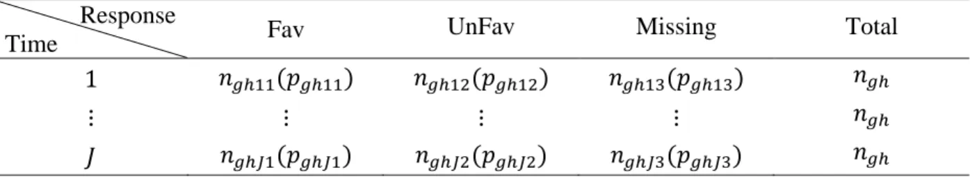
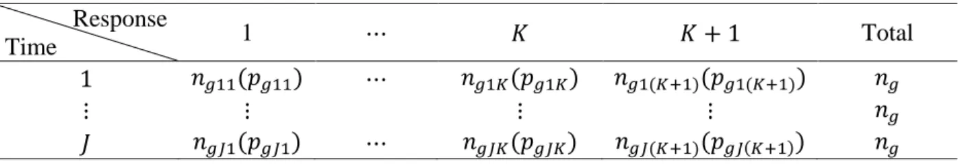
2.2.2 Data Structure
For subjects in treatment group 𝑔 and stratum ℎ, the observed data can be arranged in a contingency table format as in Table 2.1. After including missing as a category, the number of
Table 2.1 Data Structure Response
Time Fav UnFav Missing Total
1 𝑛𝑔ℎ11(𝑝𝑔ℎ11) 𝑛𝑔ℎ12(𝑝𝑔ℎ12) 𝑛𝑔ℎ13(𝑝𝑔ℎ13) 𝑛𝑔ℎ
⋮ ⋮ ⋮ ⋮ 𝑛𝑔ℎ
𝐽 𝑛𝑔ℎ𝐽1(𝑝𝑔ℎ𝐽1) 𝑛𝑔ℎ𝐽2(𝑝𝑔ℎ𝐽2) 𝑛𝑔ℎ𝐽3(𝑝𝑔ℎ𝐽3) 𝑛𝑔ℎ
subjects at each visit is fixed as 𝑛𝑔ℎ. The cell count 𝑛𝑔ℎ𝑗𝑘 is 𝑛𝑔ℎ𝑗𝑘 = ∑ 𝑦𝑔ℎ𝑖𝑗𝑘 𝑛𝑔ℎ
𝑖=1 , and cell proportion 𝑝𝑔ℎ𝑗𝑘 is 𝑝𝑔ℎ𝑗𝑘 =𝑛𝑔ℎ𝑗𝑘
𝑛𝑔ℎ𝑗 = (𝑛𝑔ℎ𝑗1, 𝑛𝑔ℎ𝑗2, 𝑛𝑔ℎ𝑗3), which follows a multinomial distribution,
𝒏𝑔ℎ𝑗~𝑀𝑢𝑙𝑡𝑖𝑛𝑜𝑚𝑖𝑛𝑎𝑙(𝑛𝑔ℎ, 𝝅𝑔ℎ𝑗), where 𝝅𝑔ℎ𝑗 = (𝜋𝑔ℎ𝑗1, 𝜋𝑔ℎ𝑗2, 𝜋𝑔ℎ𝑗3) ′
is the marginal
multinomial probability vector of response for the 𝑗-th visit. From the properties of multinomial distributions, the unbiased estimator of the multinomial probability 𝝅𝑔ℎ𝑗, is the proportion vector at row 𝑗, 𝒑𝑔ℎ𝑗 = (𝑝𝑔ℎ𝑗1, 𝑝𝑔ℎ𝑗2, 𝑝𝑔ℎ𝑗3)
′
. Combining across all time points, 𝒑𝑔ℎ =
(𝒑𝑔ℎ1′ , … , 𝒑𝑔ℎ𝐽′ )′ and 𝝅𝑔ℎ = (𝝅𝑔ℎ1′ , … , 𝝅𝑔ℎ𝐽′ )′ apply to the correlated multinomial distributions for the 𝒏𝑔ℎ𝑗 for the 𝐽 visits. The estimated covariance matrix of 𝒑𝑔ℎ as the mean of the 𝒀𝑔ℎ𝑖∗∗ is shown in (2.1).
𝑽𝑝𝑔ℎ = 1
𝑛𝑔ℎ(𝑛𝑔ℎ − 1)∑(𝒀𝑔ℎ𝑖∗∗− 𝒑𝑔ℎ)(𝒀𝑔ℎ𝑖∗∗− 𝒑𝑔ℎ) ′ 𝑛𝑔ℎ
𝑖=1
(2.1)
2.2.3 Favorable Probability Estimation
Now the estimation of interest is for the probability of favorable outcome. For this purpose, the missing response category is redistributed to the favorable and unfavorable outcomes according to a missing outcome specification.
Let 𝑞𝑔ℎ𝑗 be the probability estimator that a subject in group g and stratum h would have a favorable outcome at visit 𝑗. The redistributed favorable outcome proportion under a missing completely at random (MCAR) specification is shown in (2.2).
𝑞𝑔ℎ𝑗 = 𝑝𝑔ℎ𝑗1+ 𝑝𝑔ℎ𝑗1
𝑝𝑔ℎ𝑗1+ 𝑝𝑔ℎ𝑗2𝑝𝑔ℎ𝑗3 (2.2)
𝑞𝑔ℎ𝑗 = 𝑝𝑔ℎ𝑗1
𝑝𝑔ℎ𝑗1+ 𝑝𝑔ℎ𝑗2 (2.3)
2.2.4 Sensitivity Analysis
So far we have assumed the missing responses are MCAR-like. However, in clinical trials, the discontinued patients could have withdrawn from the study due to reasons related to the unobserved outcome, which renders the data non-ignorable missing (NMAR); see Little and Rubin (2014).
For the subsequent discussion in this section, we omit the notation for group 𝑔 and stratum ℎ for simplicity of presentation, although they can always be included without loss of generality. Now let 𝑛𝑗1, 𝑛𝑗2, and 𝑛𝑗3 represent the counts of the favorable, unfavorable, and missing responses at visit 𝑗, and 𝑛𝑗1+ 𝑛𝑗2+ 𝑛𝑗3 = 𝑛𝑗. We further divide the missing counts 𝑛𝑗3 into 𝑛𝑗31 and 𝑛𝑗32, where 𝑛𝑗31 and 𝑛𝑗32 represent the unobserved counts with a favorable and unfavorable outcome if missing responses were actually observed. Also, 𝑝𝑗1, 𝑝𝑗2, and 𝑝𝑗3 are the corresponding proportion estimators. Thus, we have the data structure shown in Table 2.2. Also, Table 2.2 could be expanded to account for counts for two or more reasons for missing
responses.
Table 2.2 Data Structure for Missing Counts Redistribution
Visit Fav UnFav Missing Total
j 𝑛𝑗1 𝑛𝑗2 𝑛𝑗3 = 𝑛𝑗31+ 𝑛𝑗32 𝑛𝑗
The odds ratio ratio 𝜃𝑗 comparing the favorable to the unfavorable outcome in the
patients with missing status versus observed patients is shown in (2.4); and the solution it implies for 𝑛𝑗31 is shown in (2.5).
𝜃𝑗 =𝑛𝑗31 𝑛 /
𝑛𝑗1
𝑛𝑗31 = 𝜃𝑗𝑛𝑗1𝑛𝑗3
𝜃𝑗𝑛𝑗1+ 𝑛𝑗2 (2.5)
Thus, there can be determination of total favorable outcome counts through an assumed specification of the odds ratio 𝜃𝑗. Also, separate 𝜃𝑗’s could address two or more reasons for missing responses.
If 𝜃𝑗 = 1, the missing responses are assumed to be MCAR-like; if 𝜃𝑗 > 1 the missing responses are regarded as more likely to have better outcome than those observed; if 𝜃𝑗 < 1, the missing responses are regarded as more likely to have worse outcome, as is often the case for patients who discontinue the test treatment. Through adjusting for different 𝜃𝑗, different specifications of the possible outcomes for the missing response can be obtained, and thus we call the 𝜃𝑗 the sensitivity parameters for missingness.
The adjusted favorable proportion estimator can be expressed in terms of the observed proportions for the responses and the 𝜃𝑗 as shown in (2.6).
𝑞𝑗𝜃 = 𝑛𝑗1+ 𝑛𝑗31
𝑛𝑗 =
1
𝑛𝑗(𝑛𝑗1+
𝜃𝑗𝑛𝑗1
𝜃𝑗𝑛𝑗1+ 𝑛𝑗2𝑛𝑗3) = 𝑝𝑗1+
𝜃𝑗𝑝𝑗1
𝜃𝑗𝑝𝑗1+ 𝑝𝑗2𝑝𝑗3 (2.6)
By construction, the 𝑞𝑗𝜃 are comparable to what might be expected by random multiple imputation of the missing responses via (2.5), but they are alternatively produced from
mathematical redistribution as in (2.5). From (2.6), it follows that the adjusted odds of favorable versus unfavorable outcome at time 𝑗 has the structure shown in (2.7).
𝑞𝑗𝜃 1 − 𝑞𝑗𝜃 =
𝑛𝑗1(𝜃𝑗𝑛𝑗1+ 𝑛𝑗2+ 𝜃𝑗𝑛𝑗3) 𝑛𝑗2(𝜃𝑗𝑛𝑗1 + 𝑛𝑗2+ 𝑛𝑗3)
=𝑝𝑗1(𝜃𝑗𝑝𝑗1+ 𝑝𝑗2+ 𝜃𝑗(1 − 𝑝𝑗1− 𝑝𝑗2))
=𝑝𝑗1(𝑝𝑗2+ 𝜃𝑗(1 − 𝑝𝑗2))
𝑝𝑗2(𝜃𝑗𝑝𝑗1+ (1 − 𝑝𝑗1)) (2.7)
If 𝜃𝑗=1, which is the MCAR-like case, 𝑞𝑗𝜃 1−𝑞𝑗𝜃 =
𝑝𝑗1
𝑝𝑗2, with this indicating that the adjusted
odds of favorable outcome versus unfavorable is the same as the odds for the observed outcomes.
2.2.5
Covariance Matrix EstimationLet 𝒒𝜃 = (𝑞1𝜃, … , 𝑞𝐽𝜃) denote the 𝑗-dimensional vector of adjusted outcome proportion estimators. In order to use the linear Taylor series methods discussed in Koch et al. (1977), as well as summarized Stokes et al. (2012, Chapter 14), to produce a consistent estimate for the covariance matrix of the adjusted proportion vector 𝒒𝜽, we express 𝒒𝜽 in the form of compound functions of the unadjusted proportion vector 𝒑 = (𝒑1′, … , 𝒑𝐽′)′ and sensivity parameter 𝜃 as shown in (2.8).
𝒒𝜽 = 𝑨𝟑𝒆𝒙 𝒑[𝑨𝟐𝒍𝒐𝒈(𝑨𝟏𝜽𝒑)] (2.8)
In (2.8), log() denotes the element-wise vector operation that transforms a vector to the corresponding vector of natural logarithms, and exp [] denotes the element-wise vector operation that transforms a vector to the corresponding vector of exponentiated values, and matrices 𝑨𝟏𝜽, 𝑨𝟐, and 𝑨𝟑 are shown in (2.9) for which 𝒃𝒅𝒊𝒂𝒈𝑱(𝑳𝒋) denotes a diagonal matrix of J blocks, with
𝑨𝟏𝜽= 𝒃𝒅𝒊𝒂𝒈𝑱(
1 0 0 𝜃𝑗 0 0 𝜃𝑗 1 0 0 0 1
) , 𝑨𝟐= 𝒃𝒅𝒊𝒂𝒈𝑱(1 0 0 0
0 1 − 1 1) , 𝑨𝟑 = 𝒃𝒅𝒊𝒂𝒈𝑱(1 1) (2.9)
𝑽𝑞𝜃 = 𝑩𝜃𝑽𝒑𝑩𝜃′ (2.10)
For (2.10), 𝑩𝜃 is the elementwise first partial derivative of vector 𝒒𝜽 with respect to vector 𝒑 and is obtained by applying the chain rule, as shown in (2.11) for which 𝒂𝟏𝜽 = 𝑨𝟏𝜽𝒑,
𝑩𝜽 = 𝝏𝒒𝜽
𝝏𝒑 = 𝝏𝒒𝜽 𝝏𝒂𝟑𝜽
𝝏𝒂𝟑𝜽 𝝏𝒂𝟐𝜽
𝝏𝒂𝟐𝜽 𝝏𝒂𝟏𝜽
𝝏𝒂𝟏𝜽
𝝏𝒑 = 𝑨𝟑𝑫𝒂𝟑𝜽𝑨𝟐𝑫𝒂𝟏𝜽
−𝟏𝑨
𝟏𝜽 (2.11)
𝒂𝟐𝜽 = log (𝒂𝟏𝜽), 𝒂𝟑𝜽= exp [𝑨𝟐𝒂𝟐𝜽], and 𝒒𝜽 = 𝑨𝟑𝒂𝟑𝜽, and 𝑫𝒂−𝟏𝟏𝜽 is a diagonal matrix with the reciprocals of the elements of the vector 𝑎1𝜃 on the main diagonal and 𝑫𝒂𝟑𝜽 is the diagonal matrix with the elements of the vector 𝒂𝟑𝜽 on the main diagonal.
Now we reconsider group 𝑔 and stratum ℎ, for which the adjusted favorable proportion estimate is shown in (2.12).
𝑞𝑔ℎ𝑗𝜃 = 𝑝𝑔ℎ𝑗1+
𝜃𝑗𝑝𝑔ℎ𝑗1
𝜃𝑗𝑝𝑔ℎ𝑗1+ 𝑝𝑔ℎ𝑗2𝑝𝑔ℎ𝑗3 (2.12)
The covariance estimate of 𝒒𝒈𝒉𝜽, where 𝒒𝒈𝒉𝜽= (𝑞𝑔ℎ1𝜃, … , 𝑞𝑔ℎ𝐽𝜃)′ is shown in (2.13). 𝑽𝒒𝒈𝒉𝜽 = 𝑩𝒈𝒉𝜽𝑽𝒑𝒈𝒉𝑩𝒈𝒉𝜽
′ (2.13)
The selection of the sensitivity parameter 𝜃𝑔ℎ𝑗 could be based on knowledge for the trial being conducted and the nature of disease; see Zhao et al. (2014). In many cases, it can
correspond to fractions of the reciprocal for a known odds ratio for the effect of a useful treatment versus placebo.
2.2.6 Treatment Comparison Treatment Difference
The treatment difference Δ = (Δ1, ⋯ , Δ𝐽) between test and placebo visits 1 to 𝑗 could be estimated using the corresponding adjusted proportion differences, and they can be weighted by the Mantel-Haenszel weights 𝑤ℎ = { 𝑛1ℎ𝑛2ℎ⁄(𝑛1ℎ+𝑛2ℎ)
∑𝐻ℎ′=1𝑛1ℎ′𝑛2ℎ′⁄(𝑛1ℎ′+𝑛2ℎ′)} for the combined strata. The
treatment difference estimator at visit 𝑗 for Δ𝑗 is 𝑑𝑗𝜃 as shown in (2.14).
𝑑𝑗𝜃 = ∑ 𝑤ℎ(𝑞1ℎ𝑗𝜃− 𝑞2ℎ𝑗𝜃) 𝐻
ℎ=1
(2.14)
Letting 𝒅𝜽= (𝑑1𝜃, ⋯ , 𝑑𝐽𝜃), the consistent covariance matrix estimator of 𝒅𝜽 can be obtained using the covariance matrix estimator 𝑽𝒒𝒈𝒉𝜽 of 𝒒𝒈𝒉𝜽 in (2.13), and it is expressed as (2.15).
𝑽𝒅𝜽 = ∑ 𝑤ℎ
2(𝑽
𝒒𝟏𝒉𝒋𝜽+ 𝑽𝒒𝟐𝒉𝒋𝜽)
𝐻
ℎ=1
(2.15)
Adjusted Treatment Difference via Randomzation-Based ANCOVA
In a randomized clinical trial, baseline covariables are expected to have the same distribution in the randomized groups. Baseline covariables could include the baseline measurement of the outcome, demographic variables, or other variables. However, random imbalances in the baseline covariables could occur as each treatment group is a finite sample of the randomized population, and covariance adjustment for them can offset such imbalances.
estimate that is associated with the imbalance would be corrected to offset the direction of the imbalance. The estimation is through randomization-based ANCOVA, which is an approach that applies weighted least squares methods to evaluate differences between treatment groups with respect to outcome variables and covariables simultaneously (Koch et al., 1998).
Here, we introduce some notations for the covariables. Suppose each subject has 𝑀 baseline covariables 𝒙𝒈𝒉𝒊, 𝒙𝒈𝒉𝒊 = (𝑥𝑔ℎ𝑖1, … , 𝑥𝑔ℎ𝑖𝑀)′, and 𝒙̅𝒈𝒉 = 1
𝑛𝑔ℎ
∑𝑛𝑖=1𝑔ℎ𝒙𝒈𝒉𝒊 is the mean
vector of the prespecified covariables. We define 𝒇𝒈𝒉𝒊 = (𝒀𝒈𝒉𝒊∗∗′ , 𝒙𝒈𝒉𝒊′ )
′
as a (3 × 𝐽 + 𝑀) dimensional response-covariable vector, and 𝒇̅𝒈𝒉= 1
𝑛𝑔ℎ∑ 𝒇𝒈𝒉𝒊
𝑛𝑔ℎ
𝑖=1 = (𝒑𝒈𝒉′ , 𝒙̅𝒈𝒉′ ) ′
is the mean of the response-covariable vector.
Further, we transform 𝒇̅𝒈𝒉 to 𝑭𝒈𝒉𝜽= (𝒒𝒈𝒉𝜽′ , 𝒙̅𝒈𝒉′ )′, then 𝑭𝒈𝒉𝜽 = (𝑨𝟑𝐞𝐱𝐩[𝑨𝟐𝐥𝐨𝐠(𝑨𝟏𝜽𝒑𝒈𝒉)] , 𝒙̅𝒈𝒉′ )
′ .
Also, we denote 𝒖 = ∑𝐻ℎ=1𝑤ℎ(𝒙̅1ℎ− 𝒙̅2ℎ) as the covariable difference weighted across the 𝐻 strata and combine the J treatment differences and 𝑀 covariable difference to get 𝑮𝜽 = (𝒅̂𝜃′, 𝒖′)′.
The consistent covariance matrix estimator 𝑽𝒇̅𝒈𝒉 of 𝒇̅𝒈𝒉 can be obtained as in (2.16).
𝑽𝒇̅𝒈𝒉 = 1 𝑛𝑔ℎ(𝑛𝑔ℎ− 1)
∑(𝒇𝒈𝒉𝒊−𝒇̅𝒈𝒉)(𝒇𝒈𝒉𝒊−𝒇̅𝒈𝒉)′ 𝑛𝑔ℎ
𝑖=1
(2.16)
And then the covariance matrix 𝑉𝐹𝑔ℎ𝜃 of 𝐹𝑔ℎ𝜃 and 𝑉𝐺𝜃 of 𝐺𝜃 can be obtained as (2.17) and (2.18).
𝑽𝑭𝒈𝒉𝜽 = [𝑩𝒈𝒉𝜽 𝟎𝑱,𝑴
𝟎𝑴,𝟑𝑱 𝑰𝑴 ] 𝑽𝒇̅𝒈𝒉[
𝑩𝒈𝒉𝜽′ 𝟎𝟑𝑱,𝑴
𝑽𝑮𝜽 = ∑ 𝑤ℎ2(𝑽𝑭𝟏𝒉𝜽 + 𝑽𝑭𝟐𝒉𝜽) 𝐻
ℎ=1
(2.18)
Then the differences between means for covariables for the two treatment groups are restricted to zero, as is expected by randomization of patients to the two treatments; this constraint can be expressed as shown in (2.19).
𝑬(𝒖) = 𝟎𝑴 (2.19)
Randomization-based covariable adjustment for the treatment comparison estimator 𝒅𝜃 with respect to 𝒖 can be invoked by fitting the linear model in (2.20) by weighted least squares
𝐸(𝑮𝜽) ≜ [0𝐼𝐽
𝑀,𝐽] 𝒃𝜽 = 𝒁𝒃𝜽=
( 𝒃1𝜃
⋮ 𝒃𝐽𝜃
0 ⋮ 0 )
(2.20)
regression with weights based on 𝑉𝐺−1𝜃 in (2.18) and with “≜” meaning “is estimated by.” The weighted least squares regression for the specification in (2.20) produces the estimator for the covariable-adjusted treatment comparisons 𝒃𝜽 in (2.21), with a consistent estimator for the covariance matrix of 𝒃𝜽, as in (2.22).
𝒃𝜽 = (𝒁′𝑽𝑮𝜽
−𝟏𝒁)−𝟏𝒁′𝑽 𝑮𝜽
−𝟏𝑮
𝜽 (2.21)
𝑽𝒃𝜽= (𝒁
′𝑽 𝑮𝜽
−𝟏𝒁)−𝟏 (2.22)
Hypothesis Testing
corresponding estimator 𝒅𝜽 or covariable-adjusted estimator 𝒃𝜽, and 𝑪 is the desired full rank contrast matrix with rank 𝑟(𝑪). Under 𝐻0, 𝑄𝑪𝚫~𝜒𝑟(𝑪)2 when the sample size is sufficiently large, where 𝜒𝑟(𝑪)2 is the central Chi-square distribution with 𝒓(𝑪) degrees of freedom.
Example
The proposed method for sensitivity analysis is illustrated with an example of a double-blind, randomized, placebo-controlled, parallel-group study to assess the safety and efficacy of a test medicine for weight loss in obese patients. The sample data consist of 1000 patients in a bootstrap sample from an obesity trial like that discussed in Smith et al. (2010).
One of the co-primary endpoints of this weight loss study is the proportion (%) of patients who achieve ≥5% weight loss from baseline to week 52. The study participants were followed every 4 weeks until the end of the study. The primary assessment was body weight at Week 52, and other important assessment visits were at Week 12, Week 24, and Week 36. These 4 visits are numbered Visits 1 to 4 in chronological order.
Substantial numbers of patients withdrew from the study and didn't return for follow up. In this bootstrap sample, at Week 52, 45.5% and 53.1% of patients had missing responses for the test and placebo group respectively; at all visits, more missingness happened in the placebo group than in the test group, as shown in Table 2.3.
Table 2.3 Missing Percentages of Assessment Visits Visit
Group 1 2 3 4
Test 10.9% 28.8% 38.5% 45.5%
Two strata according to gender were considered; and baseline weight, age, and baseline body mass index (BMI) were covariables with adjustment through randomization-based
ANCOVA as discussed in Section 2.2.6.
One question of regulatory interest for this example is whether there are 15% or more responders for test treatment than placebo. If missing responses cannot be assumed to be
ignorable, how robust the results are if challenged by a sequence of sensitivity parameters 𝜃 is a question of interest.
The hypotheses are 𝐻0𝑗: 𝑰𝒋,𝟒𝚫 ≤ 15% versus 𝐻𝐴𝑗: 𝑰𝒋,𝟒𝚫 > 15% for 𝑗 = 1, 2, 3, 4 of the 4 visits, where 𝑰𝒋,𝟒 denote the 𝑗𝑡ℎ row of the identity matrix 𝑰𝟒, and it will be addressed with the direct treatment difference estimator and the covariables-adjusted treatment difference estimator respectively. For sequential testing to address multiplicity, the primary assessment Visit 4 𝐻04 would be addressed as a first step with two-sided hypothesis testing at the 𝛼 = 0.05 level, and if significant, 𝐻03 would be addressed, etc.
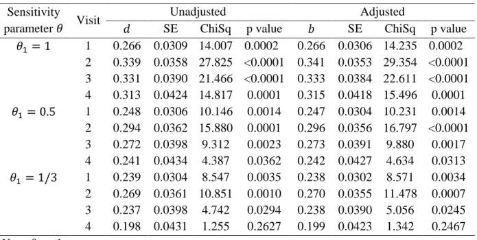
significance level of 0.05), although the attention can additionally be given to the point estimate and confidence interval. The estimates of unadjusted and adjusted treatment differences, and their standard errors (SE), and the Chi-Square values and corresponding p-values of the testing for the hypothesis 𝐻0 above are listed in Table 2.4.
Table 2.4 Results of Sensitivity Analyses for Treatment Comparison Estimators Sensitivity
parameter 𝜃 Visit
Unadjusted Adjusted
𝑑 SE ChiSq p value 𝑏 SE ChiSq p value
𝜃1 = 1 1 0.266 0.0309 14.007 0.0002 0.266 0.0306 14.235 0.0002 2 0.339 0.0358 27.825 <0.0001 0.341 0.0353 29.354 <0.0001 3 0.331 0.0390 21.466 <0.0001 0.333 0.0384 22.611 <0.0001 4 0.313 0.0424 14.817 0.0001 0.315 0.0418 15.496 0.0001 𝜃1 = 0.5 1 0.248 0.0306 10.146 0.0014 0.247 0.0304 10.231 0.0014 2 0.294 0.0362 15.880 0.0001 0.296 0.0356 16.797 <0.0001 3 0.272 0.0398 9.312 0.0023 0.273 0.0391 9.880 0.0017 4 0.241 0.0434 4.387 0.0362 0.242 0.0427 4.634 0.0313 𝜃1 = 1/3 1 0.239 0.0304 8.547 0.0035 0.238 0.0302 8.571 0.0034 2 0.269 0.0361 10.851 0.0010 0.270 0.0355 11.478 0.0007 3 0.237 0.0398 4.742 0.0294 0.238 0.0390 5.056 0.0245 4 0.198 0.0431 1.255 0.2627 0.199 0.0423 1.342 0.2467 Note: 𝜃2= 1
When the missingness is MCAR in either the test group or placebo group with 𝜃1 = 𝜃2 = 1, the conclusion that the test treatment had 15% or more responders than the placebo treatment
the estimates of the unadjusted difference 𝑑𝜃 and covariable adjusted difference 𝑏𝜃 are similar. And the standard errors of the adjusted difference 𝑏𝜃 estimator are only slightly smaller than those of the unadjusted 𝑑𝜃.
Discussion