arXiv:1609.09542v2 [nlin.PS] 29 Dec 2016
c
World Scientific Publishing Company
Peakompactons: Peaked compact nonlinear waves
Ivan C. Christov
School of Mechanical Engineering, Purdue University West Lafayette, IN 47907, USA
Tyler Kress
Department of Mathematics, University of North Carolina, Chapel Hill Chapel Hill, NC 27599, USA
Avadh Saxena
Theoretical Division and Center for Nonlinear Studies, Los Alamos National Laboratory Los Alamos, NM 87545, USA
Received Day Month Year Revised Day Month Year
This article is meant as an accessible introduction to/tutorial on the analytical con-struction and numerical simulation of a class of non-standard solitary waves termed
peakompactons. These peaked compactly supported waves arise as solutions to nonlinear evolution equations from a hierarchy of nonlinearly dispersive Korteweg–de Vries-type models. Peakompactons, like the now-well-know compactons and unlike the soliton so-lutions of the Korteweg–de Vries equation, have finite support,i.e., they are of finite wavelength. However, unlike compactons, peakompactons are also peaked,i.e., a higher spatial derivative suffers a jump discontinuity at the wave’s crest. Here, we construct such solutions exactly by reducing the governing partial differential equation to a nonlinear ordinary differential equation and employing a phase-plane analysis. A simple, but reli-able, finite-difference scheme is also designed and tested for the simulation of collisions of peakompactons. In addition to the peakompacton class of solutions, the general phys-ical features of the so-calledK#(n, m) hierarchy of nonlinearly dispersive Korteweg–de
Vries-type models are discussed as well.
Keywords: Peakompactons; solitons; Korteweg–de Vries equation; traveling wave solu-tions; phase plane analysis.
1. Introduction
Peakompactons, the definition of which will be made more precise below, are peaked compactly supported solutions to nonlinear evolution equations from a hierarchy of nonlinearly dispersive Korteweg–de Vries-type models. First, we motivate this class of models by reviewing some modern theories of wave propagation in generalized continua.
1.1. Motivating example: Waves in generalized continua
The governing equations for peakompactons originate from the study of waves in certain continua with an inherent length scale. Suchgeneralized continua1,2 arise in
the extension of classical continuum mechanics to the modeling of “real” materials. For example, myriads of materials ranging from metals to composites to granular media feature a “minimal” (often called inherent) length scale, be it the atomic lattice spacing, the typical size of inhomogeneities or the average grain diameter.
In 1995, Rubinet al.3 posed the question: can a simple model capture dispersion
of waves in non-ideal (generalized) continua due to an inherent length scale? Their proposed model, which is nowadays termed “Rubin–Rosenau–Gottlieb (RRG) the-ory,” inherits and satisfies all the thermodynamic restrictions on the admissibility of motions and parameters of the classical thermoviscous compressible Newtonian fluid. As a result, a self-contained constitutive equation can be obtained. Letting the total stress in the material beT=T(1)+T(2), where
T(1)=−℘I+ 2µsymm[∇u] + µB−23µ
(∇ ·u)I (1)
is the Cauchy stress of a thermoviscous compressible Newtonian fluid (see,e.g.,§15 in Ref. 4), the dispersive regularization takes the form
T(2)=̺Ψ2 symm[∇u] + 2(˙ ∇u)⊤∇u−4(symm[∇u])2 . (2)
In Eqs. (1) and (2) above,℘represents the thermodynamic pressure,̺is the fluid’s density, µ and µB are the fluid’s shear and bulk viscosities respectively, I is the identity tensor,uis the velocity vector, symm[F] = 12 F+F⊤returns the symmetric part of the tensor field F, a superscript ⊤ denotes transpose, a superimposed dot denotes the material derivative∂(·)/∂t+ (u·∇)(·), and Ψ is a parameter introduced in the RRG theory. Rubin et al.3 term Ψ, which is positive and has the units of
length squared, the dispersion function. It is further assumed that Ψ can depend only on the rate of deformation tensor’s second invariant, namely the scalar δ = symm[gradu] : symm[gradu].
Constitutive relations of the form T = T(1) + T(2), with T(1) and T(2) given by Eqs. (1) and (2), share some general features with models such as the so-called second-grade fluid of Coleman & Noll,5,6 the Navier–Stokes-α mod-els in turbulence,7,8,9 Lagrangian-averaged Euler-αmodels,10,11,12,13 finite-scale theories,14,15,16,17 etc. Under all of these formulations, the governing system of flow equations is modified to include an inherent length scale, which is meant to model some desired physical effect or, often, attempts to capture (in a simple way) a number of “subgrid” (or, unmodeled) effects.
Recently,18,19,20 it has been of interest to combine the RRG constitutive re-lation with the usual continuum balances of mass and linear momentum (in the absence of body forces), namely,4
˙
̺+̺∇ ·u= 0, (3a)
and to derive (unidirectional)nonlinear evolution equations for waves in these gener-alized continua. Specifically, by standard methods,21,22 Destrade & Saccomandi18 obtained a one-dimensional (1D) dimensionless equation for unidirectional propaga-tion of weakly-nonlinear shear waves in a hyperelastic, incompressible solid, under the assumption that Ψ∝(symm[∇u])3,
vt+12(v3)x+13[(vx)3]xx= 0, (4)
wherev is a strain. Henceforth, xandtsubscripts stand for partial differentiation with respect toxandt. (Although solitons are often associated with waves in fluids, and above we only reviewed the RRG theory in the context of fluids, an excellent overview of the history of and context for solitary wave propagation in elastic solids is given by Maugin.23) Meanwhile, Jordan & Saccomandi,19 also working in 1D, ob-tained a dimensionless equation for unidirectional propagation of weakly-nonlinear acoustic waves in an inviscid, non-thermally conducting compressible fluid, under the assumption that Ψ∝(symm[∇u])2,
ut+ǫbuux+16a1[(ux)3]xx= 0, (5)
whereuis a velocity,ǫis a Mach number,bis the so-called coefficient of nonlinearity of the fluid,24 anda1 is related to the material dispersion length scale
√
Ψ. Here, it should also be noted, however, that some anomalous behaviors of wave propagation under the RRG theory have been observed when viscosity is taken into account25 [unlike in Eq. (5), which is derived forinviscid fluids]. Notice that the relationship between the advective nonlinearities in Eqs. (5) and (4), namely uux versusv2vx, is precisely the same as for the Korteweg–de Vries (KdV) and themodified KdV26 equations.
Surprisingly, it has been shown recently27 that Eqs. (4) and (5) belong to a sin-gle hierarchyof generalized KdV-like nonlinearly dispersive partial differential equa-tions (PDEs) withHamiltonian structure. (It goes without saying that Hamiltonian structure is highly desirable as it underpins all of classical and modern mechan-ics of both point particles and continua, including wave phenomena and evolution equations.28,29,30,31) In the present context, the KdV equation, first introduced by Boussinesq32 and later re-derived and examined in detail by Korteweg & de Vries,33 takes the form
ut+uux+uxxx= 0, (6)
when properly normalized. Since the seminal discovery of elastic interactions of soli-tons by Zabusky & Kruskal34 (see also Refs. 35, 36), the KdV equation has been a staple ofnonlinear science.37 The key difference between Eq. (6) and Eqs. (4) and (5) is in the last term on their respective left-hand sides. While, Eq. (6) features the
and science, it behooves us to understand such “straightforward” (and physically relevant) nonlinearly dispersive extensions of KdV as the ones given in Eqs. (4) and (5) above.
1.2. K#(n, m): A nonlinearly dispersive KdV hierarchy
To summarize the derivation from Ref. 27, consider the properly normalized La-grangian density for the generic (1 + 1)-dimensional fieldϕ=ϕ(x, t):
L(ϕ;x, t) =1 2ϕxϕt+
1
(n+ 2)(n+ 1)(ϕx) n+2
−m1+ 1(ϕxx)m+1, n, m >0, (7)
where the Lagrangian density corresponding to the classical KdV equation is the special case n = m = 1.39 The corresponding action functional is RdxdtL. It is extremized by requiring that the fieldϕsatisfies the Euler–Lagrange equation (see,
e.g.,§11 and§35 in Ref. 40):
∂L ∂ϕ− ∂ ∂t ∂L ∂ϕt −∂x∂
∂L ∂ϕx + ∂ 2 ∂x2 ∂L ∂ϕxx
= 0. (8)
Substituting Eq. (7) into Eq. (8), we obtain the governing nonlinear evolution equa-tion
K#(n, m) : ut+unux+ [(ux)m]xx= 0, u(x, t)≡ϕx(x, t), (9)
where we have introduced the notation “K#(n, m)” to represent this two-parameter family of PDEs. It is evident that Eq. (4) [K#(2,3)] and Eq. (5) [K#(1,3)], which were derived to describe waves in the generalized RRG continua with an inherent length scale, are special cases of Eq. (9), subject to proper normalization ofu.27
As expected from Noether’s theorem,41 three conserved quantities (i.e., quan-tities that areconstant during thetime evolution of the fieldϕ) exist27 for Hamil-tonian equations of the form given in Eq. (9), namely
H≡
Z +∞
−∞
dxH=
Z +∞
−∞ dx
−(n+ 2)(1n+ 1)un+2+ 1
m+ 1(ux) m+1
, (10a)
M ≡
Z +∞
−∞
dx ∂L ∂ϕt
=1 2
Z +∞
−∞
dx ϕx=1 2
Z +∞
−∞
dx u, (10b)
P≡ −
Z +∞
−∞
dx ∂L ∂ϕt
ϕx=−1 2
Z +∞
−∞
dx(ϕx)2=−12 Z +∞
−∞
dx u2. (10c)
Here, H, M and P denote the Hamiltonian (total energy), total wave mass and total wave momentum42 associated with the field ϕ. Note that the Hamiltonian densityHis found via the Legendre transformation,43 namelyH=∂ϕ∂Ltϕt− L. The three quantities in Eq. (10) are conserved as a result of the translational invariance in space (x7→x+x0for any constantx0), translation invariance in time (t7→t+t0 for any constantt0), and shift invariance of the field (ϕ7→ϕ+ϕ0 for any constant
ϕ0). It has been shown27 thatnoother conserved quantities of the formR +∞ −∞ dx u
k,
The remaining details of the canonical structure corresponding to such Hamil-tonian PDEs (including Poisson brackets, etc.) can be built-up by following the derivations by Cooperet al.44 (see also the discussion in the next subsection).
1.3. Relationship between the K#(n, m) hierarchy and other nonlinearly dispersive KdV-like equations
Here, it is worth extending the discussion from Ref. 27 on the connection between theK#(n, m) hierarchy introduced in Section 1.2 above and previous models from the literature. For example, in a classic paper from 1993, Rosenau & Hyman45 introduced a simple model of a nonlinearly dispersive set of KdV-like equations:
K(n, m) : ut+ (un)x+ (um)xxx= 0. (11)
This set of equations initiated the study ofcompactons,i.e., solitary waves of com-pact support (equivalently, “finite wavelength”), which has led to an explosion of research on the subject.45,46,47,48,49,50,51,52 For example, in the case ofn=m= 2 [K(2,2)], the exact solution for a compacton is45
u(x, t) =
0, −∞< x−ct≤ −2π,
4 3ccos2
1
4(x−ct)
, −2π < x−ct <+2π,
0, +2π≤x−ct≤+∞.
(12)
Clearly, u(x, t) is nonzero only on a finite (moving) interval |x−ct| < 2π. Addi-tionally,u(x, t) is solely a function of the moving-frame coordinatex−ct, wherec
is the speed of the compacton. Finally, just as for the KdV “sech2” soliton,36 the compacton’s amplitude, 4c/3, depends on its speed,c.
Unfortunately, since the K(n, m) family of PDEs is based on an ad-hoc mod-ification of the KdV equation, it does not preserve KdV’s Hamiltonian structure. Cooperet al.44 generalized Rosenau & Hyman’s model45 to
K∗(l, p) : u
t+ul−2ux+upuxxx+ 2pup−1uxuxx+12p(p−1)up−2(ux)3
| {z }
= 0. (13)
TheK∗(l, p) generalization of theK(n, m) equations restores Hamiltonian structure to the model. Equation (13) extremizes the action generated by the Lagrangian density
LK∗(ϕ;x, t) =1
2ϕxϕt+ 1
l(l−1)(ϕx) l
−12(ϕx)p(ϕxx)2. (14)
Just like theK(n, m) equations, theK∗(l, p) equations possess a variety of compact solitary wave solutions.44,53,54 The equivalent of the K(2,2) compacton solution given in Eq. (12) is the following (quite similar) solution to theK∗(3,1) equation:44
u(x, t) =
0, −∞< x−ct≤ −√3π,
3ccos2h√1
12(x−ct) i
, −√3π < x−ct <+√3π,
0, +√3π≤x−ct≤+∞.
Evidently, the difference between the K(n, m) and K∗(l, p) equations is the “weights” of the expanded nonlinearly dispersive term. Specifically, notice that the terms grouped by an under-brace in Eq. (13) are the same as in the expansion of the term (um)xxx (with m= p+ 1) in Eq. (11) but with different coefficients! Meanwhile, the difference between the Lagrangian densities in Eqs. (14) and (7) is in how the dispersive term is modified,i.e., from∝(ϕxx)2for KdV to∝(ϕxx)m+1for
K#(n, m) to∝(ϕx)p(ϕxx)2 forK∗(l, p). This difference has a profound impact on the structure of traveling wave solutions, as we explore in detail in Section 2 below. Specifically, simple explicit compacton solutions of the form given in Eqs. (12) and (15) are not available for theK#(n, m) equations.
More recently, a version of the K∗(l, p) family of equations, which is invariant under the joint action of parity reflection and time reversal (the so-called PT -symmetric extension55 of real-valued PDEs56), has been introduced by Benderet al.,57 yielding a hierarchy of equations of the form
K∗
PT(l, p, r) : ut+ul−2ux−
p r−1[u
p−1(ux)r]x+ r
r−1[u
p(ux)r−1]xx= 0, (16)
where the third parameterris necessary to ensurePT-invariance. The correspond-ing Lagrangian is57,58
LK∗
P T(ϕ;x, t) =
1 2ϕxϕt+
1
l(l−1)(ϕx) l
−(r1 −1)(ϕx)
p(ϕxx)r. (17)
Evidently, in introducing thePT-symmetric version of the K∗(l, p) equations, and the new parameterr, an “interpolation” between the originalK∗(l, p) equations and theK#(n, m) equations is obtained! Specifically, we see that, upon proper rescaling ofϕ, xand t, the subset ofK∗
PT(l, p, r) equations (16) with p= 0 can be mapped onto theK#(n, m) equations (9), for appropriately chosen landr.
2. Construction of traveling wave solutions
A goal of the present work is to discuss some exact results regarding solutions of the
K#(n, m) hierarchy of equations. The plan of attack is to first reduce the PDE (9) to an ordinary differential equation (ODE) and, then, to study the structure of the latter’s solutions.
2.1. Reduction to an ODE and its integration
Let ξ = x−ct be moving-frame coordinate for some speed c > 0 (i.e., a right-propagating wave). Then, we suppose that the solution to Eq. (9) can be expressed in the form of atraveling wave, specificallyu(x, t) =U(ξ). Substituting thisansatz
into Eq. (9), we arrive at the ODE:
ξto yield:
−cU+ 1
n+ 1U
n+1+(U′)m′=C
1, (19)
whereC1is an arbitrary constant of integration. Next, we multiply Eq. (19) byU′ and rewrite all terms as complete derivatives:
−c2 U2′+ 1
(n+ 1)(n+ 2) U
n+2′+ m
m+ 1
(U′)m+1′=C1U′. (20)
Integrating a second time and rearraning, we arrive at
(U′)m+1=C2+ Ψ[U;C1, κ, γ], (21)
where
Ψ[U;C1, κ, γ]≡C1U+κU2−γUn+2, (22)
and, for convenience, we have introduced
κ≡(m+ 1)
2m c, γ≡
(m+ 1)
(n+ 1)(n+ 2)m. (23)
Taking the (m+ 1)st root of both sides of Eq. (21) and separating variables yields anexact but implicit relation betweenξandU:
Z dU
(C2+ Ψ[U])1/(m+1)
=±ξ+ξ0, (24)
whereξ0is the final integration constant. The ambiguity introduced by the ‘±’ sign on the right-hand side of Eq. (24) is due to the multi-valued nature of the (m+ 1)st root; choosing a branch cut, for example, fixes the sign, but both signs are valid. One obvious restriction that must be applied in arriving at Eq. (24) is that
C2+ Ψ[U]≥0 (25)
for allU in the (currently unspecified) integration interval, for given values ofC2,
C1, κ and γ. Hence, allowable limits of integration in Eq. (24) can fall between consecutive zeros ofC2+ Ψ[U] and/or±∞, as long as the condition in Eq. (25) is satisfied.
More generally, solutions to Eq. (21) correspond tointegral curvesin the (U, U′) phase plane.59 Certain valuesU =U∗ such that
C2+ Ψ[U∗;C1, κ, γ] = 0 ⇔ U′|U=U∗ = 0 (26)
solutions such that |U(ξ)| <∞ ∀ξ, on physical grounds.) One consequence of this interpretation is thatξ plays the role of “time of flight” along an integral curve in the (U, U′) phase plane. Hence, if two equilibriaU =U∗
1,2 can be reached along an integral curve in finite “time,” the solutions in the ξ, U(ξ) plane are such that
U(ξ)6=U∗
1,2 only on afinite (in other words,compact) interval ofξ.
Finally, note that Eq. (18) admits “anti” solutions propagating to the left (i.e., the ODE remains invariant) under the transformationU → −U and c→ −c only if n+ 1 andmare even.
Let us now illustrate the ideas discussed in this subsection in some special cases.
2.1.1. C1=C2= 0
Consider the case in which the first two integration constants are forced to vanish,
i.e., C1=C2= 0. Then, Eq. (21) becomes
(U′)m+1=U2(κ−γUn). (27)
Clearly, there are two equilibria in this case:
U∗
1 = 0, U2∗= κ
γ 1/n
=1
2(n+ 1)(n+ 2)c 1/n
. (28)
Notice thatunless C2= 0, thenU1∗= 0cannot be an equilibrium. We shall return to the case ofC16= 0 in Section 2.1.2.
A peakompacton will thus be a traveling wave solution that connects the two equilibria in Eq. (28). To construct our desired traveling wave solution, we now fix one of the limits of integration in Eq. (24) to be an equilibrium point (specifically, it is convenient to set the lower limit toU∗
1 = 0) to obtain:
Z U
0
d ˆU h
ˆ
U2κ−γUˆni1/(m+1)
=±ξ+ξ0, (29)
where ˆU is the “dummy” integration variable. Upon judicious inspection of the integrand (or using the computer algebra system Mathematica), we find that the integral above is one of the integral representations of Gauss’ hypergeometric function2F1(a, b;c;z).60 With some effort, Eq. (29) evaluates to
m+ 1
m−1
U(m−1)/(m+1)
κ1/(m+1)
2F1
1
m+ 1,
m−1
(m+ 1)n; 1 +
m−1
(m+ 1)n; γ κU
n
=±ξ+ξ0.
(30) We must ensure that this solution does indeed pass through the two equilibria given in Eq. (28). By construction, the left-hand side of Eq. (30) already goes to 0 asU →U∗
1, hence we must have thatξ→ ∓ξ0 on the right-hand side. This clearly means that the U∗
1 equilibrium can be reached in finite ξ! Then, by translation invariance, we are free to require that U → U∗
Enforcing this last condition,
ξ0=
m+ 1
m−1
(U∗
2)(m−1)/(m+1)
κ1/(m+1)
2F1
1
m+ 1,
m−1
(m+ 1)n; 1 +
m−1
(m+ 1)n; 1
,
(31) whereU∗
2 = 1
2(n+ 1)(n+ 2)c 1/n
as given in Eq. (28). Thus, the complete peakom-pacton traveling wave solution is
U(ξ) =
0, −∞< ξ≤ −ξ0,
inverse of Eq. (30), −ξ0< ξ <0, 1
2(n+ 1)(n+ 2)c 1/n
, ξ= 0,
inverse of Eq. (30), 0< ξ <+ξ,
0, +ξ0≤ξ≤+∞.
(32)
Clearly, this peakompacton islocalized in the “usual” sense of solitons, specifically
U(ξ)→0 as|ξ| → ∞and, hence,u(x, t)→0 as|x| → ∞ (t <∞).
The reason we are allowed to piece (or, “glue”) together the non-zero solution in Eq. (30) with the equilibrium solutionU =U∗
1 = 0 at the (finite) pointsξ=±ξ0 is that, at those points, the Lipschitz condition (see,e.g., Chapter 5,§8 in Ref. 61) required for theuniquenessof solutions of an ODE is violated. This violation is also evident from Eq. (27), in which solving forU′involvesfractional powers of the right-hand side; fractional roots are generally not Lipschitz functions. Therefore, many solutions to this nonlinear ODE can be constructed, in particular the peakompacton in Eq. (32) (see also the discussion in Refs. 18, 19, 62, 63, 64).
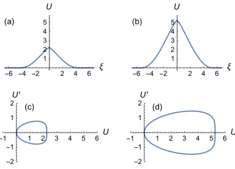
From Eq. (32), it is clear that the amplitude,U∗
2, of the peakompacton is solely a function ofn(the power of the advective nonlinearity). Meanwhile,m(the power of the dispersive nonlinearity) only affects the width, 2ξ0, of the peakompacton. The wave speed c changes both the amplitude and width through U∗
2. Figure 1 shows the peakompacton solution ofK#(1,3) for (a) c= 0.75 (“subsonic”) and (b)
c= 1.75 (“supersonic”). As is typical for nonlinear waves, such as the KdV “sech2” soliton36 and compactons,45,44 the peakompacton’s amplitude is a function of its speedc.
2.1.2. C16= 0,C2= 0
In this case, Eq. (21) becomes
(U′)m+1=C1U+U2(κ−γUn). (33)
Now, there can be up ton+ 2 equilibria (zeros of the right-hand side), with one of them beingU∗
1 = 0, which clearly persists. By Descartes’ rule of signs, however, if
Fig. 1. The peakompacton solution of theK#(1,3) equation for (a)c= 0.75 (⇒ξ
0≈4.27) and
(b)c= 1.75 (⇒ξ0≈5.28), constructed via Eq. (32). Panels (c) and (d) show the corresponding
phase plane portraits of the peakompactons from panels (a) and (b).
for these roots. In the special case ofn= 1, we use the quadratic formula to obtain
U1∗= 0, U2∗,3=
κ±p4C1γ+κ2
2γ (n= 1). (34)
Similarly, Cardano’s formula yields a closed-form expression forn= 2, however, it is too lengthy to list here.
A qualitative analysis of the phase plane of Eq. (33) [shown in Fig. 2(c)] reveals that when C1 > 0 (i.e., when U2∗ < 0 < U3∗), a peakompacton connecting U1∗ and U∗
3 can be constructed. However, in this case, the solution turns out to be an anti-peakompacton, which travels on a “level,” as illustrated in Fig. 2(a). A lengthy calculation shows that, although there does not appear to be a closed-form solution (even implicit) for arbitraryn, the special case of n= 1 is amenable to further manipulation, and an implicit solution can be constructed for the wave profile connectingU∗
1 andU3∗:
m+ 1
m
[(κ−s)U+ 2C1][(κ+s)U+ 2C1] 4C2
1[C1+U(κ−γU)]U
1/(m+1)
U
×F1
m m+ 1;
1
m+ 1, 1
m+ 1; 2− 1
m+ 1; 2γU κ+s,
2γU κ−s
=±ξ (n= 1), (35)
where we have sets≡p4γC1+κ2 for convenience, andF
vanishes asU →U∗
1 = 0, hence we have set ξ0 = 0 to center the traveling wave at
ξ= 0.
Fig. 2. Nonstandard peakompacton solutions of theK#(1,3) equation with c = 0.75 for (a)
C1 = 0.1 (⇒ U3∗ ≈ 2.43), constructed by piecing together the solution in Eq. (35) and the
equilibriumU∗
3 from Eq. (34), and (b) C1 = −0.1 (⇒U2∗ ≈0.22,U3∗ ≈2.02), constructed by
piecing together numerical solutions of Eq. (33) and the equilibriumU∗
2 from Eq. (34). Panels (c)
and (d) show the corresponding phase plane portraits of the peakompactons from panels (a) and (b).
In the case when both equilibria U∗
2,3 > 0 [i.e., −κ2/(4γ) < C1 < 0], we can once again construct a peakompacton connectingU∗
2 to U3∗. In this case, we found difficulties adapting the solution given in Eq. (35). However, numerical integration (usingMathematica’sNDSolvesubroutine) of Eq. (21) starting fromU∗
2 allows us to compute the wave profile, which is now a peakompacton traveling on a “level,” as illustrated in Fig. 2(b).
2.1.3. C1= 0,C26= 0
In this case, Eq. (21) becomes
(U′)m+1=C
2+U2(κ−γUn). (36)
The most pernicious feature of having C1 = 0 andC2 6= 0 is thatU = 0 is no longer an equilibrium, which was always the case in Sections 2.1.1 and 2.1.2. By Descartes’ rule of signs, if C2<0, then the right-hand side of Eq. (36) has only a single positive root. Therefore, forC2<0, a peakompacton solution does not exist. On the other hand, it is easy to see that the case ofC2>0 is qualitatively similar to the case of C2 = 0 and C1 < 0 from Section 2.1.2, so we will not dwell on it further.
2.1.4. Other cases
It is certainly conceivable that even more traveling wave constructions, for special values of the integration constants C1, C2 and the exponents n, m, are possible. We do not claim the discussion above exhausts all possibilities. However, the cases considered above do illustrate a breadth of possible “exotic” traveling wave solutions to theK#(n, m) hierarchy of equations.
For example, periodic solutions of arbitrary spatial period ℓ ≥ 2ξ0, where [−ξ0,+ξ0] is the interval of compact support of the solutions above, can always be constructed from identical peakompactons (i.e., samen, mandc). This super-position property follows immediately from the compactness (finite wavelength) of the peakompacton traveling waveforms of theK#(n, m) hierarchy of equations.
2.2. Regarding derivative discontinuities
Although the class of solutions derived in Section 2.1.1 (C1=C2= 0) is implicit, it is still possible to obtain results regarding the derivativesU′(ξ) andU′′(ξ) of the traveling wave profile. The key fact is that asξ→ ±ξ0,U →(U1∗)+ and asξ→0,
U →(U2∗)−. Then, from Eq. (27), we obtain
U′(ξ)→ (
0, ξ→0,
0, ξ→ ±ξ0.
(37)
Therefore, U′(ξ), likeU(ξ) itself, is continuous atξ ={0,±ξ
0} and, hence, for all
ξ∈R.
Then, by implicit differentiation, Eq. (27) also allows us to compute
U′′(ξ) = {2κ−(n+ 2)γ[U(ξ)] n}U(ξ)
(m+ 1) ([U(ξ)]2{κ−γ[U(ξ)]n})(m−1)/(m+1). (38)
Once again, considering the limitsξ→ ±ξ0[U →(U1∗)+] andξ→0 [U →(U2∗)−], a preliminary analysis of discontinuities ofU′′(ξ) can be performed; see§4 of Ref. 27. To summarize:
|U′′(ξ)| →
0, ξ→ ±ξ0 (0< m <3), p
c/6, ξ→ ±ξ0 (m= 3),
∞, ξ→ ±ξ0 (m >3),
∞, ξ→0 (∀m >0).
Jump discontinuities of finite size in the higher derivatives of a function [U(ξ) in the present context] are termedmild discontinuities.66,67 More severe discontinu-ities in the higher derivatives (i.e., the derivatives approach±∞or are undefined) are also possible according to Eq. (39). Specifically, higher derivative discontinuities at thecrest of a wave play an important role in the classification of “exotic” trav-eling wave solutions of nonlinear evolution equations. Another classical nonlinearly dispersive equation, which we have not mentioned so far, is the Camassa–Holm (CH) equation:68,69,70,71
ut+ 3uux−2uxuxx+uuxxx=uxxt, (40)
which has the following traveling wave solution:
u(x, t) =U(ξ) =ce−|ξ|, ξ≡x−ct. (41)
The solution given in Eq. (41) is termed a peakon because U′(ξ) suffers a finite jump (mild discontinuity) at ξ = 0, while U′′(ξ) is undefined there (due to the presence of a Diracδ-function inU′′). Although Eq. (40) is not exactly a nonlinearly dispersive KdV-like equation due to the mixed-derivative term, the CH equation also possesses a rich geometrical structure,72,28 including beingbi-Hamiltonian68,69,71 and related to umbilic geodesics on surfaces.73 [Interestingly, a change of signs in Eq. (40) can lead to an integrable bi-Hamiltonian equation that admits compacton solutions.74]
Figure 3 qualitatively illustrates various solitary wave solutions of dispersive evolution equations and their derivatives. The KdV “sech2” soliton36 (a) isC∞(R) (infinitely continuously differentiable). The K(2,2) profile45 (b) is C1(R) (once continuously differentiable), since U′′ suffers jumps at the edges of the compact support. TheK#(1,3) profile27 (in the case ofC
1=C2= 0 from Section 2.1.1) (c) isC1(R) as well, withU′′ suffering jumps at the edges of the compact support and
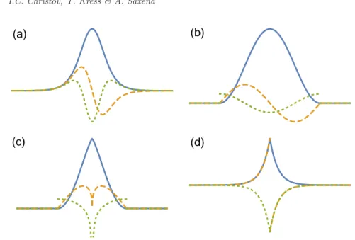
U′′ blowing up at ξ = 0. Finally, the CH profile68 (d) is onlyC0(R) because U′ suffers a jump atξ= 0, andU′′is undefined there. The important observation here, in particular as far as the terminology is concerned, is that the classical (KdV) soliton is infinitely smooth, while compactons exhibit mild discontinuities at the edges of their compact support. Meanwhile, peakons suffer mild discontinuities at the crest of the wave. Peakompactons exhibit both the features of peakons and compactons, hence theportmanteau“peakompacton.”
In passing, we also make note of a completely integrable75 evolution
equa-tion (unlike the, presumably, non-integrable compacton and peakompacton hier-archies discussed above) that admits piecewise linear solutions, namely the Hunter– Saxton76 equation:
(ut+uux)xx=12 u2x
x, (42)
Fig. 3. Illustrations of the traveling wave solutions of four nonlinearly dispersive evolution equa-tions: (a) KdV, (b)K(2,2), (c)K#(1,3), and (d) CH. While the horizontal scales are the same in
all four panels, the vertical scales have been adjusted for clarity;c= 1 in all panels. Axes are not shown in order to clearly highlight onlyqualitativefeatures. In each panel, solid curves represent the traveling wave profileU(ξ), dashed curves representU′(ξ), and dotted curves representU′′(ξ).
Note that in panel (c) the vertical axis does not show the full range andU′′(ξ)→ −∞, in fact. In
panel (d), the Diracδ-function inU′′(ξ) cannot be visualized, of course.
can be constructed. Although such solutions are conceptually related to our discus-sion, Eq. (42) is fundamentally of a different type than the KdV-like nonlinearly dispersive equations that are the subject of this work. A conceptually closer type of nonlinearly dispersive evolution equation is the Harry Dym equation:38
ut=u3uxxx. (43)
This equation, like the CH equation, admits peakon solutions and is also completely integrable by the inverse scattering transform, which brings about connections to the KdV equation.77
Finally, we acknowledge that the possibility of infinite second derivatives techni-cally means that the solutions considered herein are (in a sense)weak solutions,i.e., they do not possess as many continuous derivatives as are present in the governing ODE. There are a number of mathematical issues that must be elucidated for such
pseudo-classical78,79,80 (orsingular81) solutions. For further details, the reader is
terms have finite limits as ξ→ {0,±ξ0}, so that the ODE itself does not suffer a jump discontinuity at those points (see also the discussion in Ref. 57).
2.3. Explicit variational approximations
In the previous subsections, we discussed the structure of theexact traveling wave reduction of theK#(n, m) equations. Clearly, the structure of the associated ODE is nontrivial. Furthermore, the exact solutions we found were implicit and involved hypergeometric special functions. In this subsection, we would like to ask the ques-tion: can explicit approximations to the traveling wave solutions of the K#(n, m) hierarchy of equations given in Eq. (9), i.e., approximate solutions of the ODE in Eq. (18), be obtained?
To answer this question, we appeal to the so-called method ofvariational approx-imation82,83,84,85 (see also Refs. 86, 87 for discussion of the method’s accuracy).
The idea of the variational approximation is that, for a given properly parametrized explicit functional form of the traveling wave solution U(ξ), from which u(x, t) and ϕ(x, t) follow of course, the variational structure of the governing PDE pro-vides a natural way to determine “optimal” choices of the free parameters in the parametrized approximation. This technique is best illustrated through an example. Ideally, a parametrized explicit functional form, or ansatz, for peakompactons would itself also be compact. We could introduce a trial function of the form
U(ξ)≈U˜(ξ;t) =
(
A(t)eb(t)/(|ξ|−ξc),
|ξ|< ξc, 0, |ξ| ≥ξc,
(44)
where A(> 0) and b(> 0) are to be determined as part of the procedure, ξ ≡
x−ct is the moving-frame coordinate as before, andξc is the half-length of the compact support [e.g.,ξ0as given in Eq. (31) for the peakompactons constructed in Section 2.1.1]. The key idea is to now computeϕ(x, t) on the basis of Eq. (44) and, then, substitute the expression into the Lagrangian densityL(ϕ;x, t) from Eq. (7). The next step is to compute R−∞+∞dxL to obtain the Lagrangian itself. Because the calculated Lagrangian is based on an ansatzand is no longer a function of x, we term it thecoarse-grained Lagrangian88 L(A,b;t). Now, Lgenerates an action functional, which we must require to be stationary with respect to variations ofA andb. Hence, two coupled ODEs can be obtained, which determine the “optimal” values of thea priori undetermined parameters in the trial function ˜U(ξ;t).
Unfortunately, however, when using Eq. (44) as the ansatz, the integration over x cannot be performed in terms of elementary functions. An alternative parametrized functional form is required. One way forward is to relax the require-ment that theansatzbe a compact function ofξ, and to use thepost-Gaussiantrial function:44,57,89
U(ξ)≈U˜(ξ) =Aexp−β|ξ|2η , (45)
of time. The difference between theans¨atze in Eqs. (44) and (45) is illustrated in Fig. 4.
Fig. 4. Illustration of the differences between the analytically intractable but compact ansatz
given in Eq. (44) (solid curve) and the analytically tractable but non-compactansatz given in Eq. (45) (dashed curve);A= 25.79, b= 3.25,ξc= 1 andA= 1,β = 4.5,η= 0.65. Evidently,
these twoans¨atzecan be made to agree quite well for appropriately chosen (for the purposes of this figure, “by eye”) parameters.
Integrating Eq. (45) with respect toξ, we find the functional form of the field
ϕ(x, t) = Φ(ξ) associated tou(x, t) under the traveling wave assumption:
˜
Φ(ξ) =− Aξ
2η(β|ξ|2η)1/(2η)Γ
1 2η, β|ξ|
2η
, (46)
where Γ(a, x)≡Rx+∞dζ ζ
a−1e−ζ is theincomplete Gamma function.90 To compute
R+∞
−∞ dxLbased on the Lagrangian density in Eq. (7), we note the following chain rules apply for the chosenansatz:
ϕx(x, y) = ˜Φ′(ξ)ξ
x= ˜U(ξ), ϕxx(x, t) = ˜U′(ξ), ϕt(x, t) = ˜Φ′(ξ)ξt=−cU˜(ξ). (47) Then, substituting the expressions from Eq. (47) intoR−∞+∞dxL, using the fact that dx= dξ and appealing to symmetry to rewriteR−∞+∞dξ[· · ·] = 2R0+∞dξ[· · ·], we obtain
L= 2
Z +∞
0 dξ
−c2U˜2+ 1
(n+ 2)(n+ 1)U˜ n+2
−m1+ 1 U˜′m+1
. (48)
Upon evaluating the integrals using ˜U from Eq. (45), the coarse-grained Lagrangian takes the form
L(A, β, η;n, m, c) = Γ
1 + 1 2η
2βAn+2
(n+ 1)[β(n+ 2)]1+1/(2η)−
cA2 (2β)1/(2η)
+ (−1)m
(2A)m+1(βη)mΓh1− 1 2η
m+ 1i
(m+ 1)2[β(m+ 1)][1−1/(2η)]m . (49)
This expression for L is valid only for η such that m < 2η(m+ 1), otherwise the integral definingL does not converge. Now, we extremize the function of three variables (all of which are independent of time) given in Eq. (49), namely we require that the following simultaneous equations hold:
∂L
∂A = 0, ∂L
∂β = 0, ∂L
∂η = 0
. (50)
The resulting solutions for A,β and η in terms of each other and n,m and c are lengthy (see also the discussion in§IV in Ref. 44). To illustrate the variational ap-proximation, however, let us restrict to the two featured equations from Section 1.1, namelyK#(1,3) andK#(2,3). Furthermore, let us fix the wave speed to bec= 0.75 (a “subsonic” peakompacton). Then, the three conditions in Eq. (50) yield
(A, β, η)≈ (
(2.21423,0.310367,0.822982), (n, m, c) = (1,3,0.75),
(2.09741,0.428176,0.774748), (n, m, c) = (2,3,0.75). (51)
For completeness, note that the system in Eq. (50) is a non-trivial set of tran-scendental equations coupling A, β and η. This system is amenable by numerical methods only. In practice, it is useful and possible to first solve∂L/∂β= 0 explic-itly for β in terms of Aand η (as well as n,m andc, of course). Then, the latter solution is substituted into the remaining two equations, which can then be solved numerically usingMathematica’sFindRootsubroutine.
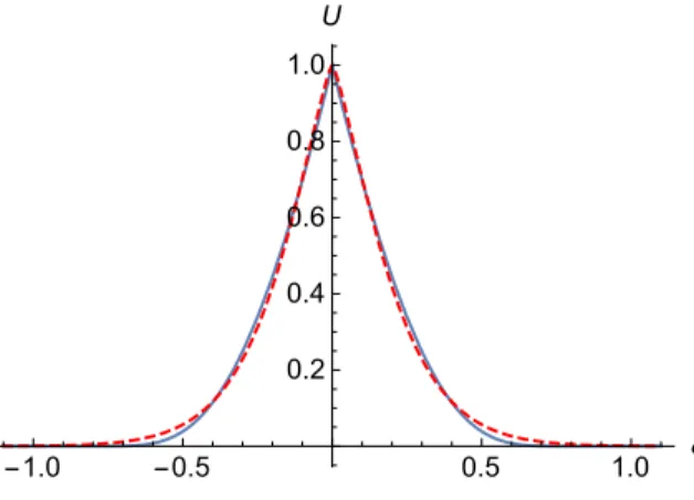
A comparison between the exact peakompacton solutions and their variational approximations is shown in Fig. 5; the agreement is quite good away fromξ=±ξ0, where the non-compact ansatz in Eq. (45) is not expected to be a good approxi-mation. Note that maxξU(ξ) =U∗
2 ≡ 1
2(n+ 1)(n+ 2)c 1/n
[recall Eq. (28)], which gives maxξU(ξ) = 2.25 for (n, m, c) = (1,3,0.75) and maxξU(ξ) ≈ 2.12132 for (n, m, c) = (2,3,0.75). On comparing these values to the correspondingA values given in Eq. (51), we see that the variational approximation is accurate to≈1.5%. Finally, once the optimal values of A, β and η have been computed for given
n,mand c, the total energy, wave mass and wave momentum can easily be found from Eqs. (10) based on theansatzgiven in Eq. (45):
H =
(−1)m+1(2A)m+1(βη)mΓh1− 1 2η
m+ 1i
(m+ 1)2[β(m+ 1)][1−1/(2η)]m −
2βAn+2Γ1 + 1 2η
(n+ 1)[β(n+ 2)]1+1/(2η), (52a)
M = A
β1/(2η)Γ
1 + 1 2η
, (52b)
P =− A
2
(2β)1/(2η)Γ
1 + 1 2η
Fig. 5. Comparison between the exact peakompacton solutions [i.e., Eq. (32), solid curves] of the (a)K#(1,3) and (b)K#(2,3) equations and their variational approximations [i.e., Eqs. (45) and
(51), dashed curves].
As before, the expression forHis valid only forηsuch thatm <2η(m+1), otherwise the integral defining H does not converge.
3. Numerical solution of peakompacton equations
Now, we turn to the numerical solution of theK#(n, m) equations given in Eq. (9). Our purpose in obtaining numerical solutions to the “full” PDE is to simulate and shed light on the interactions of multiple peakompactons.
Previously Pad´e approximation methods,91,92,93,94 finite difference95,96 and fi-nite element methods,97 particle methods,98 the discontinuous Galerkin method,99 and the method of lines100 have all been used successfully to simulate the evolution of compactons and related KdV-like equations. Here, we use simple finite-difference methods101,102 (reminiscent of those used in the original compacton simulations45) to make the simulation of peakompactons accessible to students and those who are only beginners in numerical mathematics. However, we do warn the reader that there are many intricate details regarding the high-resolution simulation of com-pacton collisions that have been discussed in detail in the literature,103,104,105 and the reader should be aware of them when attempting to simulate peakompacton collisions.
3.1. A leap-frog scheme with filtering
We begin the construction of our numerical scheme by firstsemi-discretizing Eq. (9) using central differences in space:
duj dt =−
2 3D0
h 1 (n+1)(uj)
n+1i+1 3(uj)
nD 0[uj]
+D2[(D
0[uj])m]
| {z }
≡Lh[uj]
, (53)
solve Eq. (9) on the finite domain [−L, L] with periodic boundary conditions, i.e.,
u(−L, t) =u(L, t)∀t≥0.
In Eq. (53), we have employed the difference operators
D0[uj]≡ −
uj+2+ 8uj+1−8uj−1+uj−2
12∆x , (54)
which is the fourth-order-accurate central difference approximation to∂u/∂x (see Table 2.6 of Ref. 102), and
D2[uj]≡ −uj+2+ 16uj+112(∆−30ux)j2+ 16uj−1−uj−2, (55)
which is the fourth-order-accurate central difference approximation to ∂2u/∂x2 (again, see Table 2.6 of Ref. 102). Here, one can “plug-in” one’s favorite higher-order central difference formulæ for the first and second derivative as well. Addi-tionally, we have split the nonlinear advective termunu
x into the equivalent form 2
3[ 1 (n+1)u
n+1]x+1 3u
nu
x for improved conservation of the quadratic invariant of u,
i.e., the total wave momentumP given in Eq. (10c). The linear invariant ofu,i.e., the total wave massM given in Eq. (10b) is automatically conserved by virtue of using spatial central difference operators in Eq. (53).
Next, we must choose an appropriate time discretization for the semi-discrete system in Eq. (53). Following Hyman,106 we discretize the time derivative using an
explicitthree-level predictor–corrector method (of second-order accuracy) known as “leap-frog 2–3”:
u∗j =ukj + 2∆tLh[ukj+1] (predictor), (56a)
ukj+2 =15
ujk+ 4ukj+1+ 4∆tLh[ujk+1] + 2∆tLh[u∗j] (corrector), (56b)
where ∆t is a fixed time-step size, ukj ≈ u(xj, tk) and tk = k∆t. This time-integration scheme has desirable stability properties in that it includes portions of the imaginary axis for finite ∆t (unlike the traditional leap-frog scheme).106 Since Eq. (9) includes dispersive terms, we expect that the discrete spatial operator
Lh in Eq. (53) to have imaginary and complex eigenvalues, hence our choice of the leap-frog 2–3 scheme for the time discretization.
As mentioned above, the time-stepping scheme in Eq. (56) is athree-level scheme. To initialize it, we use the FTCS (forward-time central-space) scheme,i.e., we per-form an initialization time step by discretizing the left-hand side of Eq. (53) using the forward Euler scheme:
duj dt ≈
u1 j−u0j
∆t =Lh[u
0
j], (57)
whereu0
j is the initial condition evaluated on the computational grid.
Finally, following Cooperet al.,89 we stabilize the numerical method with low-order filtered artificial viscosity by modifying the discrete spatial differential oper-ator as follows
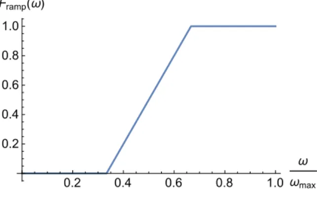
where ν∆x is the artificial viscosity. Since the artificial viscosity scales with ∆x, it vanishes as ∆x → 0, hence this modification does not affect the scheme’s con-sistency. Here, ramp spectral filter{ · } is ahigh-pass filter that takes the fast Fourier transform (inx) of its argument, then multiplies by 0 the lowest third of the Fourier modes, multiplies by 1 the highest third of the Fourier modes, and “ramps” the middle third (as illustrated in Fig. 6), before fast inverting back to real space. Artificial viscosity helps improve the stability of the numerical method by damping high-frequency numerical (aliasing) errors arising from the higher-derivative discon-tinuities of peakompactons. The spectral filtering step no longer allows us toprove
that M is conserved automatically, however, we observe in all simulations that M
is conserved to better than 1%.
Fig. 6. Fourier space representationFramp(ω) of the “ramp” spectral filter used to define the
artificial viscosity in Eq. (58) for the numerical scheme.
Finally, we expect that such an explicit scheme will be stable only under a Courant–Friedrichs–Lewy (CFL) condition (see,e.g.,§1.6 in Ref. 101):
∆t=CCFL(∆x)3, (59)
for some CFL numberCCFL≤1. The reason ∆xis taken to the third power is that the highest spatial derivative in the PDE (9) is of third order.
3.2. Example: an overtaking collision in K#(1,3)
In the spirit of the work of Zabusky & Kruskal,34 we would like to now establish whether peakompactons can “survive” overtaking collisions, and, if so, whether this type of collision is elastic. To this end, we restrict to the case ofn= 1 andm= 3,
i.e., the K#(1,3) equation. We generate an initial condition that consists of two peakompactons of disjoint support and different wave speedsc1and c2:
whereU(ξ) is given by Eq. (32). The peakompactons comprising the initial condition are shifted byξ1andξ2with respect to the origin of the coordinate system to ensure their supports do not overlap and to give them enough distance to propagate before reaching the (periodic) downstream boundary at x = L. Then, the full initial– boundary–value problem is solved using the finite-difference scheme constructed in Section 3.1.
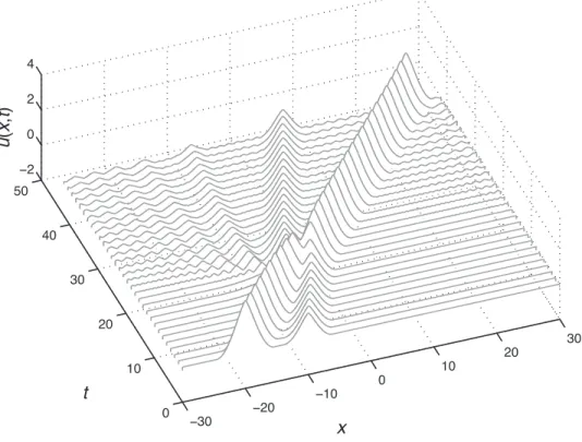
Our featured simulation is presented in Fig. 7 in the form of a “waterfall” space-time plot. In this simulation, we have takenL = 30, tfinal = 42, ∆x = 0.05 (⇒
N = 1201), ∆t is determined via the CFL condition (59) with CCFL = 0.1, and
ν = 3. For the initial condition’s parameters, we have used ξ1 = −10, c1 = 0.5,
ξ2 =−20 andc2 = 1. Throughout the simulation, we monitored the evolution of the invariants M, P and H from Eq. (10) and found thatM is conserved within 0.03%. Meanwhile, P and H are conserved within 3.7% and 4.7%, respectively. Furthermore, doubling the grid size did not change the qualitative features of the interaction, which we describe below. Hence, we have a degree of confidence in the quality and reproducibility of the numerical simulation shown in Fig. 7.
In the space-time plot presented in Fig. 7, we observe that the two peakom-pactons were initially placed so that the faster (therefore, taller) is on the left and
−30
−20
−10 0
10
20
30
0 10 20 30 40 50
−2 0 2 4
x
t
u
(
x
,
t
)
the slower (therefore, shorter) is on the right att= 0. Since peakompactons prop-agate to the right, this setup results in an overtaking collision in which the taller collides with and advances past the shorter peakompacton. This is evident in the space-time plot by visually tracking the initial peaks. Clearly, the two peakom-pactons survive the collision and continue to propagate “unharmed.” However, the collision is not purely elastic as radiation modes (and possibly newly generated peakompactons) emerge from the moment of interaction, which occurs shortly after
t= 20. Aside from these radiation modes, the space-time plot in Fig. 7 is quite typ-ical of soliton collisions in the KdV equation (see, e.g., Fig. 3.3 in Ref. 37). Thus, so far, we can conclude peakompactons appear to be stable objects that can collide and retain their identity. But, the presence of further propagation modes emerging from the collisions leads us to term the collision asnearly elastic.
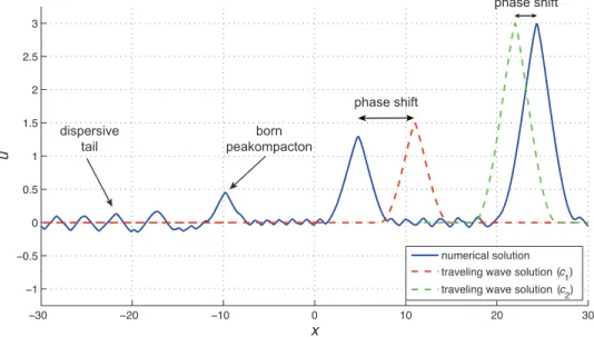
To further elucidate the dynamics of the overtaking collision, in Fig. 8, we show
u(x, tfinal) as a function of x(solid curve), while the would-be current location of each individual peakompacton, had it propagated by itself (undisturbed), is shown by a dashed curve. Clearly, the final locations of the interacting peakompactons differ from those of the undisturbed ones. This difference in location is termed a
phase shift. The taller one is ahead, while the shorter one is behind. Furthermore, while the taller peakompacton appears to have preserved its shape identically, the
−30 −20 −10 0 10 20 30
−1 −0.5 0 0.5 1 1.5 2 2.5 3
x
u
numerical solution
traveling wave solution (c
1)
traveling wave solution (c
2)
phase shift
phase shift
born peakompacton dispersive
tail
Fig. 8. Snapshot of the wavefield after an overtaking collision of two peakompactons. This figure shows the finalt-trace from the spacetime plot in Fig. 7 withu(x, tfinal) as a solid curve and the
shorter peakompacton is markedly even shorter. We conjecture that this is due to the “birth” of a third, trailing peakompacton at the moment of interaction. Furthermore, the self-similar dispersive tail seen in Fig. 7 is clearly depicted in Fig. 8. The tail has apparently reached the left end of the periodic domain (x=
−L), thus oscillations from it can be observed throughout the whole domain. The emergence of a self-similar dispersive pulse, which could be termed an Airy pulse, from the collision of two peakompactons is reminiscent of collisions in higher-order compacton equations89 and of collisions of “sech2” pulses in the Korteweg–de Vries– Kuramoto–Sivashinsky–Velarde (KdV–KSV) equation,107 which is a higher-order KdV-like equation incorporating both viscous and hyperviscous terms as well as Marangoni effects. Finally, we do note that further numerical experiments suggest that the features of the collision just described, namely that (i) the peakompactons “survive” the collision, (ii) a third peakompacton is “born” and (iii) a dispersive tail is generated, are robust.
4. Conclusion
equation,85 theφ6equation,108 the sine-Gordon equation88,109 and the nonlinear Schr¨odinger equation,110 there are ways to extract important collision information from the coupled set of ODEs governing the parameters of the linear superposition of two independent instances of the variationalansatz.
Finally, an important topic that we have not mentioned at all in the present work isstability111 of the constructed traveling wave solutions as functions ofn,m, etc. Stability can be explored, to some degree, through numerical experimentation but much more can be said by analytical methods. We will not attempt to summarize the extensive literature on the topic in the limited space of the conclusion, beyond noting that this is an avenue of future work.
Acknowledgements
This work was initiated while I.C.C. and T.K. were enjoying the hospitality of the Center for Nonlinear Studies at Los Alamos National Laboratory (LANL). I.C.C. was partially supported by the LANL/LDRD Program through a Feynman Distin-guished Fellowship. LANL is operated by Los Alamos National Security, L.L.C. for the National Nuclear Security Administration of the U.S. Department of Energy un-der Contract No. DE-AC52-06NA25396. I.C.C. would also like to thank F. Cooper, D.D. Holm, J.M. Hyman, P.M. Jordan and A. Oron for helpful discussions on the topic of the present work. Last but not least, we would like to thank Surajit Sen for organizing this special issue, for inviting us to contribute and for hosting I.C.C. and A.S. at the 2016 workshop on “Nonlinear Dynamics of Many Body Systems” in Buffalo, New York, where the idea for this manuscript was finalized.
References
1. G. A. Maugin and A. V. Metrikine (eds.),Mechanics of Generalized Continua: One
Hundred Years After the Cosserats (Springer Science+Business Media, New York,
2010).
2. H. Altenbach, G. A. Maugin, V. Erofeev (eds.),Mechanics of Generalized Continua (Springer-Verlag, Berlin/Heidelberg, 2011).
3. M. B. Rubin, P. Rosenau and O. Gottlieb,J. Appl. Phys.77, 4054 (1995).
4. L. D. Landau and E. M. Lifshitz,Fluid Mechanics, 2nd ed. (Pergamon Press, Oxford, UK, 1987).
5. B. D. Coleman and W. Noll,Arch. Rational Mech. Anal.6, 25 (1960).
6. J. E. Dunn and R. L. Fosdick,Arch. Rational Mech. Anal.56, 191 (1974).
7. S. Chen, C. Foias, D. D. Holm, E. Olson, E. S. Titi and S. Wynne,Physica D133,
49 (1999).
8. C. Foias, D. D. Holm and E. S. Titi,Physica D152–153, 505 (2001).
9. J. L. Guermond, J. T. Oden and S. Prudhomme,Physica D177, 23 (2003).
10. D. D. Holm, J. E. Marsden and T. S. Ratiu,Phys. Rev. Lett.80, 4173 (1998).
11. D. D. Holm,Physica D170, 253 (2002).
12. H. S. Bhat and R. C. Fetecau,Discret. Contin. Dyn. Syst. B6, 979 (2006).
13. R. S. Keiffer, R. McNorton, P. M. Jordan and I. C. Christov,Wave Motion48, 782
14. L. G. Margolin,Phil. Trans. R. Soc. A367, 2861 (2009).
15. L. G. Margolin,Mech. Res. Commun.57, 10 (2014).
16. P. M. Jordan and R. S. Keiffer,Phys. Lett. A379, 124 (2015).
17. L. G. Margolin, inCoarse Grained Simulation and Turbulent Mixing, ed. F. F. Grin-stein (Cambridge University Press, Cambridge, UK, 2016), pp. 48–86.
18. M. Destrade and G. Saccomandi,Phys. Rev. E73, 065604 (2006).
19. P. M. Jordan and G. Saccomandi,Proc. R. Soc. A468, 3441 (2012).
20. M. B. Rubin,Proc. R. Soc. A469, 20120641 (2013).
21. A. Jeffrey and T. Kakutani,SIAM Rev.14, 582 (1972).
22. D. G. Crighton,Annu. Rev. Fluid Mech.11, 11 (1979).
23. G. A. Maugin,Mech. Res. Commun.38, 341 (2011).
24. W. Lauterborn, T. Kurz and I. Akhatov, in Springer Handbook of Acoustics, ed. T. D. Rossing (Springer Science+Business Media, New York, 2007), pp. 257–297. 25. P. M. Jordan, R. S. Keiffer and G. Saccomandi,Wave Motion51, 382 (2014).
26. R. M. Miura,J. Math. Phys.9, 1202 (1968).
27. I. C. Christov,Proc. Estonian Acad. Sci.64, 212 (2015), arXiv:1501.01044 [math-ph].
28. D. D. Holm, T. Schmah and C. StoicaGeometric Mechanics and Symmetry: From
Finite to Infinite Dimensions(Oxford University Press, New York, 2009).
29. P. J. Morrison,Rev. Mod. Phys.70, 467 (1998).
30. V. E. Zakharov and E. A. Kuznetsov,Physics–Uspekhi40, 1087 (1997).
31. P. J. Olver,Math. Proc. Camb. Phil. Soc.88, 71 (1980).
32. J. Boussinesq,M´emoires pr´es´entes par divers savants `a l’Acad´emie des Sciences de
l’Institut de FranceXXIII, 1 (1877).
33. D. J. Korteweg and G. de Vries,Phil. Mag. (Ser. 5)39, 422 (1895).
34. N. J. Zabusky and M. D. Kruskal,Phys. Rev. Lett.15, 240 (1965).
35. R. M. Miura.SIAM Rev.18, 412 (1976).
36. P. G. Drazin and R. S. Johnson, Solitons: An Introduction (Cambridge University Press, Cambridge, UK, 1989).
37. A. Scott,Nonlinear Science: Emergence and Dynamics of Coherent Structures, 2nd ed. (Oxford University Press, Oxford, UK, 2003).
38. M. Kruskal, in:Dynamical Systems, Theory and Applications, ed. J. Moser (Springer-Verlag, Berlin/Heidelberg, 1975), pp. 310–354.
39. C. S. Gardner,J. Math. Phys.12, 1548 (1971).
40. I. M. Gelfand and S. V. Fomin,Calculus of Variations(Dover Publications, Mineola, New York, 2000).
41. M. D. Kruskal and N. J. Zabusky,J. Math. Phys.7, 1256 (1966).
42. G. A. Maugin and C. I. Christov, inSelected Topics in Nonlinear Wave Mechanics, ed. C. I. Christov and A. Guran (Birkh¨auser, Boston, 2002), pp. 117–160.
43. L. D. Landau and E. M. Lifshitz,Mechanics, 3rd ed. (Butterworth-Heinemann, Ox-ford, UK, 1976).
44. F. Cooper, H. Shepard and P. Sodano,Phys. Rev. E48, 4027 (1993).
45. P. Rosenau and J. M. Hyman,Phys. Rev. Lett.70, 564 (1993).
46. P. Rosenau,Phys. Lett. A230, 305 (1997).
47. P. Rosenau and D. Levy,Phys. Lett. A252, 297 (1999).
48. P. Rosenau,Phys. Lett. A275, 193 (2000).
49. P. Rosenau,Not. AMS52, 738 (2005).
50. P. Rosenau,Phys. Lett. A356, 44 (2006).
51. F. Rus and F. R. Villatoro,Appl. Math. Comput.215, 1838 (2009).
52. P. Rosenau and A. Oron,Commun. Nonlinear Sci. Numer. Simulat.19, 1329 (2014).
54. F. Cooper, A. Khare and A. Saxena,Complexity11, 30 (2006), arXiv:nlin/0508010
[nlin.PS].
55. C. M. Bender and S. Boettcher, Phys. Rev. Lett. 80, 5243 (1998);
arXiv:physics/9712001 [math-ph].
56. C. M. Bender, D. C. Brody, J.-H. Chen and E. Furlan,J. Phys. A: Math. Theor.40,
F153 (2007); arXiv:math-ph/0610003.
57. C. M. Bender, F. Cooper, A. Khare, B. Mihaila and A. Saxena, Pramana73, 375
(2009), arXiv:0810.3460 [math-ph].
58. P. E. G. Assis and A. Fring,Pramana74, 857 (2010), arXiv:0901.1267 [hep-th].
59. H. T. Davis, Introduction to Nonlinear Differential and Integral Equations (Dover Publications, Mineola, New York, 1962).
60. A. B. Olde Daalhuis, in NIST Digital Library of Mathematical Functions, ed. F. W. J. Olver, D. W. Lozier, R. F. Boisvert and C. W. Clark, Chapter 15,
http://dlmf.nist.gov/, release 1.0.13, 2016.
61. E. A. Coddington,An Introduction to Ordinary Differential Equations, (Dover Pub-lications, Mineola, New York, 1989).
62. G. Saccomandi,Int. J. Non-Linear Mech.39, 331 (2004).
63. M. Destrade, G. Gaeta and G. Saccomandi, Phys. Rev. E 75, 047601 (2007),
arXiv:0711.4437 [physics.class-ph].
64. M. Destrade, P. M. Jordan and G. Saccomandi, EPL 87, 48001 (2009);
arXiv:1303.0953 [nlin.PS].
65. R. A. Askey and A. B. Olde Daalhuis, in NIST Digital Library of Mathematical
Functions, ed. F. W. J. Olver, D. W. Lozier, R. F. Boisvert and C. W. Clark,§16.13,
http://dlmf.nist.gov/, release 1.0.13, 2016.
66. B. D. Coleman and M. E. Gurtin,Phys. Fluids10, 1454 (1967).
67. D. Wei and P. M. Jordan,Int. J. Non-Linear Mech.48, 72 (2013).
68. R. Camassa and D. D. Holm,Phys. Rev. Lett.71, 1661 (1993).
69. R. Camassa, D. D. Holm and J. M. Hyman,Adv. Appl. Mech.31, 1 (1994).
70. J. P. Boyd,Appl. Math. Comput.81, 173 (1997).
71. R. Camassa,Discr. Contin. Dyn. Syst. B3, 115 (2003).
72. D. D. Holm, J. E. Marsden and T. S. Ratiu,Adv. Math.137, 1 (1998).
73. M. S. Alber, R. Camassa, D. D. Holm and J. E. Marsden,Proc. R. Soc. A450, 677
(1995).
74. P. J. Olver and P. Rosenau,Phys. Rev. E 53, 1900 (1996).
75. J. K. Hunter and Y. Zheng,Physica D79, 361 (1994).
76. J. K. Hunter and R. Saxton,SIAM J. Appl. Math.51, 1498 (1991).
77. W. Hereman, P. P. Banerjee and M. R. Chatterjee,J. Phys. A: Math. Gen.22, 241
(1989).
78. Y. A. Li, P. J. Olver and P. Rosenau, inNonlinear Theory of Generalized Functions, eds. M. Oberguggenberger, M. Grosser, M. Kunzinger and G. Hormann (CRC Press, Boca Raton, FL, 1999), pp. 129–145.
79. Y. A. Li and P. J. Olver,Discr. Contin. Dyn. Syst. A3, 419 (1997).
80. Y. A. Li and P. J. Olver,Discr. Contin. Dyn. Syst. A4, 159 (1998).
81. A. Geyer and V. Ma˜nosa,Nonlinear Anal. RWA31, 57 (2016).
82. T. Sugiyama,Prog. Theor. Phys.61, 1550 (1979).
83. D. Anderson,Phys. Rev. A27, 3135 (1983).
84. M. J. Rice,Phys. Rev. B28, 3587 (1983).
85. D. K. Campbell, J. F. Schonfeld and C. A. Wingate,Physica D9, 1 (1983).
86. D. J. Kaup and T. K. Vogel,Phys. Lett. A362, 289 (2007).
88. I. Christov and C. I. Christov,Phys. Lett. A372, 841 (2008); arXiv:nlin/0612005
[nlin.PS].
89. F. Cooper, J. M. Hyman and A. Khare,Phys. Rev. E64, 026608 (2001),
arXiv:patt-sol/9704003.
90. R. B. Paris, inNIST Digital Library of Mathematical Functions, ed. F. W. J. Olver, D. W. Lozier, R. F. Boisvert and C. W. Clark, Chapter 8,http://dlmf.nist.gov/, release 1.0.13, 2016.
91. F. Rus and F. R. Villatoro,Math. Comput. Simulat.76, 188 (2007).
92. B. Mihaila, A. Cardenas, F. Cooper and A. Saxena,Phys. Rev. E81, 056708 (2010).
93. B. Mihaila, A. Cardenas, F. Cooper and A. Saxena,Phys. Rev. E82, 066702 (2010).
94. A. Cardenas, B. Mihaila, F. Cooper and A. Saxena,Phys. Rev. E83, 066705 (2011).
95. A. C. Vliegenthart,J. Eng. Math.5, 137 (1971).
96. J. de Frutos, M. A. L´opez-Marcos and J. M. Sanz-Serna,J. Comput. Phys.120, 248
(1995).
97. M. S. Ismail and T. R. Taha,Math. Comput. Simulat.47, 519 (1998).
98. A. Chertock and D. Levy,J. Comput. Phys.171, 708 (2001).
99. D. Levy, C.-W. Shu and J. Yan,J. Comput. Phys.196, 751 (2004).
100. P. Saucez, A. Vande Wouwer, W. E. Schiesser and P. Zegeling, J. Comput. Appl.
Math.168, 413 (2004).
101. J. C. Strikwerda,Finite Difference Schemes and Partial Differential Equations, 2nd ed. (Society for Industrial and Applied Mathematics, Philadelphia, 2004).
102. D. R. Lynch,Numerical Partial Differential Equations for Environmental Scientists
and Engineers(Springer Science+Business Media, New York, 2005).
103. F. Rus and F. R. Villatoro, J. Comput. Phys. 227, 440 (2007); arXiv:0708.0486
[math-ph].
104. F. Rus and F. R. Villatoro,App. Math. Comput.204, 416 (2008).
105. J. Garral´on, F. Rus and F. R. Villatoro, Appl. Math. Comput. 220, 185 (2013);
arXiv:1209.1944 [math.NA].
106. J. M. Hyman, inAdvances in Computational Methods for PDEs–III, ed. R. Vichn-evetsky and R. S. Stepleman (IMACS, 1979), pp. 313–321.
107. C. I. Christov and M. G. Velarde,Physica D86, 323 (1995).
108. V. A. Gani, A. E. Kudryavtsev and M. A. Lizunova,Phys. Rev. D89, 125009 (2014);
arXiv:1402.5903 [hep-th].
109. C. D. Ferguson and C. R. Willis,Physica D119, 283 (1998).
110. H. E. Baron, G. Luchini and W. J. Zakrzewski,J. Phys. A: Math. Theor.47, 265201
(2014); arXiv:1308.4072 [hep-th].

![Fig. 5. Comparison between the exact peakompacton solutions [i.e., Eq. (32), solid curves] of the (a) K # (1, 3) and (b) K # (2, 3) equations and their variational approximations [i.e., Eqs](https://thumb-us.123doks.com/thumbv2/123dok_us/8301295.2198536/18.918.222.670.237.397/comparison-exact-peakompacton-solutions-curves-equations-variational-approximations.webp)