EFFICIENT INTERACTIVE SOUND PROPAGATION IN DYNAMIC ENVIRONMENTS
Carl Schissler
A dissertation submitted to the faculty of the University of North Carolina at Chapel Hill in partial fulfillment of the requirements for the degree of Doctor of Philosophy in the Department of
Computer Science in the College of Arts and Sciences.
Chapel Hill 2017
Approved by:
Dinesh Manocha
Ming C. Lin
Ravish Mehra
Gary Bishop
ABSTRACT
CARL SCHISSLER: Efficient Interactive Sound Propagation in Dynamic Environments (Under the direction of Dinesh Manocha)
The physical phenomenon of sound is ubiquitous in our everyday life and is an important component
of immersion in interactive virtual reality applications. Sound propagation involves modeling how sound
is emitted from a source, interacts with the environment, and is received by a listener. Previous techniques
for computing interactive sound propagation in dynamic scenes are based on geometric algorithms such as
ray tracing. However, the performance and quality of these algorithms is strongly dependent on the number
of rays traced. In addition, it is difficult to acquire acoustic material properties. It is also challenging to
efficiently compute spatial sound effects from the output of ray tracing-based sound propagation. These
problems lead to increased latency and less plausible sound in dynamic interactive environments.
In this dissertation, we propose three approaches with the goal of addressing these challenges. First, we
present an approach that utilizes temporal coherence in the sound field to reuse computation from previous
simulation time steps. Secondly, we present a framework for the automatic acquisition of acoustic material
properties using visual and audio measurements of real-world environments. Finally, we propose efficient
techniques for computing directional spatial sound for sound propagation with low latency using head-related
transfer functions (HRTF).
We have evaluated both the performance and subjective impact of these techniques on a variety of
complex dynamic indoor and outdoor environments and observe an order-of-magnitude speedup over previous
approaches. The accuracy of our approaches has been validated against real-world measurements and previous
methods. The proposed techniques enable interactive simulation of sound propagation in complex
TABLE OF CONTENTS
LIST OF TABLES . . . vii
LIST OF FIGURES . . . ix
LIST OF ABBREVIATIONS . . . xv
LIST OF SYMBOLS . . . xvi
1 Introduction . . . 1
1.1 Sound Propagation . . . 1
1.2 Motivation . . . 3
1.3 Challenges . . . 5
1.4 Thesis Statement . . . 7
1.5 Main Results . . . 7
1.5.1 Temporal Coherence for Sound Propagation . . . 7
1.5.2 Acoustic Material Classification and Optimization . . . 9
1.5.3 Low-Latency Spatial Sound for Sound Propagation . . . 10
1.6 Organization . . . 10
2 Background . . . 12
2.1 Sound Propagation . . . 12
2.1.1 Wave-based Sound Propagation . . . 12
2.1.2 Geometric Sound Propagation . . . 13
2.1.2.1 Specular Reflections . . . 13
2.1.2.2 Diffuse Reflections . . . 13
2.2 Acoustic Materials . . . 14
2.3 Sound Rendering . . . 15
2.3.1 Spatial Sound . . . 15
3 Temporal Coherence for Sound Propagation . . . 17
3.1 Introduction. . . 17
3.2 Temporal Coherence for Sound Propagation . . . 18
3.2.1 Specular Path Cache . . . 19
3.2.2 Diffuse Path Cache . . . 23
3.2.3 Impulse Response Cache . . . 28
3.2.4 Impulse Response Length . . . 32
3.3 Implementation . . . 35
3.4 Results . . . 36
3.4.1 Specular Path Cache . . . 36
3.4.2 Diffuse Path Cache . . . 39
3.4.3 IR Cache & Adaptive IR Length . . . 43
3.5 User Evaluation . . . 46
3.6 Conclusion, Limitations, and Future Work . . . 48
4 Acoustic Material Classification and Optimization . . . 50
4.1 Introduction. . . 50
4.2 Acoustic Material Classification and Optimization . . . 51
4.2.1 Visual Material Classification for Acoustics . . . 52
4.2.2 Acoustic Material Optimization . . . 56
4.3 Implementation . . . 62
4.4 Results . . . 64
4.5 User Evaluation . . . 69
4.6 Conclusion, Limitations, and Future Work . . . 71
5.1 Introduction. . . 73
5.2 Background . . . 74
5.2.1 HRTF Spatial Sound . . . 74
5.2.2 Spatial Impulse Response (SIR) Construction . . . 75
5.2.3 Spherical Harmonics and Spatial Sound . . . 77
5.3 HRTF-based Spatial Sound for Area and Volume Sources . . . 78
5.3.1 Theoretical derivation . . . 78
5.3.2 System Overview . . . 81
5.3.3 Analytical Projection . . . 83
5.3.4 Monte Carlo Projection . . . 86
5.4 Efficient Perceptual Construction of the Spatial Impulse Response . . . 89
5.4.1 Perceptual Directivity Metric . . . 89
5.4.2 Convolution with the HRTF . . . 92
5.5 Implementation . . . 93
5.6 Results . . . 95
5.6.1 Area and Volume Sources . . . 95
5.6.2 Spatial Impulse Response Construction . . . 98
5.7 User Evaluation . . . 101
5.7.1 Evaluation of Area and Volume Sources . . . 102
5.7.2 Evalution of Spatial Impulse Response Construction . . . 105
5.8 Conclusion, Limitations, and Future Work . . . 108
6 Conclusions and Future Work . . . 110
6.1 Summary of Results . . . 110
6.2 Limitations . . . 111
6.3 Future Work . . . 113
LIST OF TABLES
3.1 The main results of our specular path cache approach on four benchmark scenes with 10th-order specular reflections. We compare the performance of the na¨ıve ray-based image source method (RISM) with 10,000 and 1,000 primary rays to our approach with 1,000 rays (RISM+SPC). Our approach generates about as many propagation
paths as RISM with 10,000 rays, but has performance close to the RISM with 1,000 rays. . . 37
3.2 The main performance results of our diffuse path cache approach. We show the complexity of the various benchmark scenes, the number of sound sources, and the number of specular and diffuse reflection bounces. The diffuse path cache can be used
to compute sound propagation for diffuse reflections at interactive rates. . . 40
3.3 We highlight the primary results of our IR cache algorithm. Our approach is able to achieve interactive performance on complex scenes with dozens of sources. The IR cache uses only a few MB of memory per sound source, while the adaptive impulse
response length ensures that only audible rays are traced when the IR length changes. . . 44
4.1 The material categories and absorption coefficient data that was used in our classifica-tion approach. For each of the visual material categories, a similar acoustic material and its absorption coefficients were chosen from (Egan, 1988). For the “Ceramic” and “Plastic” categories, there was no suitable measured data available so a default
absorption coefficient of0.1was assigned for all frequencies. . . 54
4.2 This table provides the details of the four room-sized benchmark scenarios. We give the physical dimensions of each room and the geometric complexity of the 3D reconstructed mesh models after simplification, as well as the RT60values computed
from the IRs. We highlight the time spent in the material classification and the optimization algorithms, as well as the percentage of scene surface area correctly
classified. . . 64
5.1 The complexity of the scenes used to evaluate our area/volume spatial sound technique. The number of sound source shapes in each scene is specified using the notation: S=spheres, B=boxes, M=meshes. We list the estimated volume and area of all sound
sources in each scene. . . 96
5.2 The performance results of our area/volume spatial sound system. We report the com-putational load of the audio rendering thread (Render load) performing the auralization step. We report the timings for both the analytical projection (Analy. Proj.) used for spherical sources and Monte Carlo (M.C. Proj) used for box and meshes along with the filter construction cost (Filter const.). For all scenes, our approach can compute spatial sound filters in less than1millisecond. We also list the approximate time needed for the naive point-sampling approach. Point sources were sampled at a 1 meter resolution (filter computation time per point source = 0.006 ms). Our spatial sound algorithm is
5.3 The main results of our sound propagation and rendering system for the six benchmark scenes. We report the time taken for sound propagation separately from the SRIR construction time, and we compare the performance of our method to the performance of SRIR construction using per-path HRTF interpolation. Our method provides a
speedup of6.7−9.1over the previous approach. . . 99 5.4 The sources of latency in our sound propagation and rendering system. The total
latency for our system is around the 100ms latency target needed for interactive virtual
LIST OF FIGURES
1.1 A high-level overview of our material estimation, sound propagation, and spatial sound rendering pipeline. We use RGB images of the environment along with measured impulse responses to automatically estimate the acoustic materials. Then, we use sound propagation and temporal coherence techniques to efficiently compute interactive sound propagation. The resulting propagation paths and impulse responses are used by the sound rendering module to compute the final audio using convolution with a spatial
impulse response. . . 8
3.1 A high-level overview of our sound propagation technique that uses temporal coherence. We cache specular reflection paths, diffuse reflection paths and impulse responses in
order to improve the sound quality for interactive applications. . . 19
3.2 In our diffuse cache algorithm, rays leave the sound sourceS, hit a sequence of surface patches{T1(ζ1, ξ1), T2(ζ2, ξ2), T3(ζ3, ξ3)}, then hit the listenerL. Rays with dashed
paths are from previous frames, while rays with solid paths are from the current frame. Our technique groups these coherent rays together because they hit the same sequence of surface patches. The sound contribution at the listener is averaged over the time periodτ, using rays from the previous and current frames, resulting in less noise in the
impulse response compared to traditional path tracing approaches. . . 24
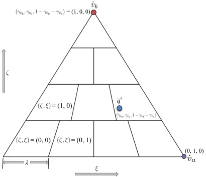
3.3 An example triangle subdivision. The triangle is subdivided into an array of indexed patches(ζ, ξ)based on the subdivision resolutionλ. We compute the ray intersection
point~qwith Barycentric coordinates(γv˙k, γv˙a,1−γv˙k−γv˙a), (e.g.(ζ, ξ) = (1,3)). . . 26 3.4 This figure summarizes our IR cache algorithm. A persistent copy of the IR,In−1, is
stored for each sound source. A small number of rays are used to compute a coarse impulse response for framen,I˜n, and this coarse IR is combined with the IR cache In−1from framen−1using the exponential smoothing factorα. The resulting filtered
IR is then stored in the IR cache for the next frame before it is used for sound rendering. . . 29
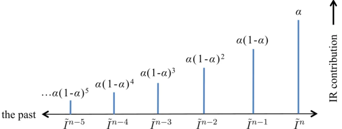
3.5 The contribution of the impulse responses from previous frames decreases for frames that are further in the past. The coarse impulse response from the current frame,I˜n, contributes with weightα, the last frameI˜n−1contributes with weightα(1−α), and
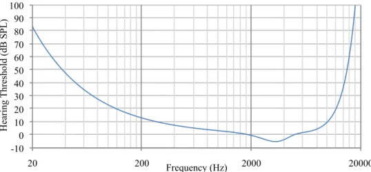
thejth previous frame with weightα(1−α)j. . . 30 3.6 Psychoacoustic Metric: The human threshold of hearing varies greatly with frequency
and is well-approximated by equation 3.8. The highest sensitivity is in the2kHz−3kHz band, and the sensitivity decreases for very low and very high frequencies. Note that
3.7 An example impulse response that shows the audible IR length for 4 frequency bands. Horizontal dashed lines correspond to the threshold of hearing for each band, and vertical dashed lines correspond to the IR length per-band. In this case, the maximum IR length over all bands is1.01s. On the next time step, rays will be propagated for up to1.01s+ ∆tp, where∆tpis a parameter that determines how much the IR length can
change per-frame. . . 34
3.8 The four benchmark scenes used to evaluate the specular path cache approach:
Audito-rium (top left), Indoor (top right), Sibenik (bottom left), Sponza (bottom right). . . 37
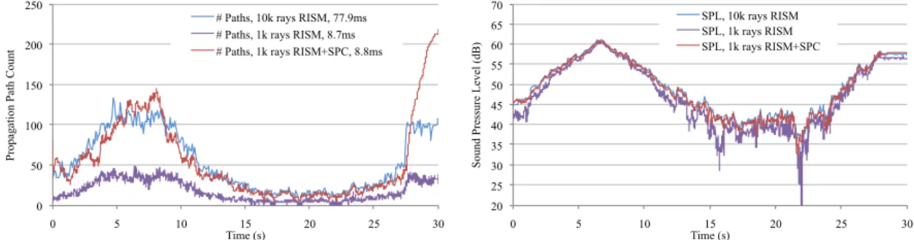
3.9 Our specular path cache (SPC) algorithm significantly improves the quality of the ray-based image source method (RISM) in terms of the number of propagation paths generated (left) and the sound pressure at the listener’s position (right) in the Sponza scene. With only 1,000 primary rays, our approach produces nearly the same output as the na¨ıve RISM with 10,000 rays, but with about the same cost as the na¨ıve RISM
with 1,000 rays. . . 38
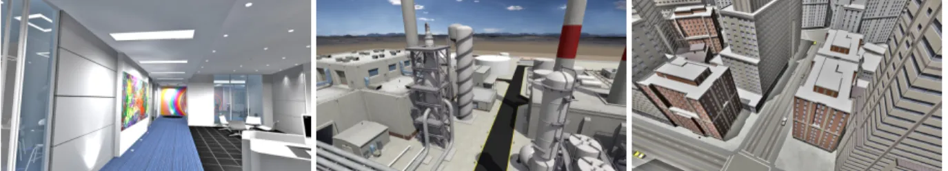
3.10 The three benchmark scenes used to evaluate our diffuse path caching algorithm. (left)
office interior (154K triangles); (center) oil refinery (245K triangles); (right) city (254K triangles). 39
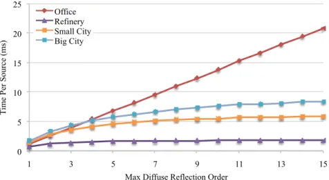
3.11 We highlight how the performance of our diffuse path cache algorithm scales with the maximum diffuse reflection order on a single CPU thread. Note that in outdoor scenes, most rays escape the scene after the 4th or 5th bounce. In the indoor office scene, the
complexity is linear with respect to the maximum diffuse order. . . 40
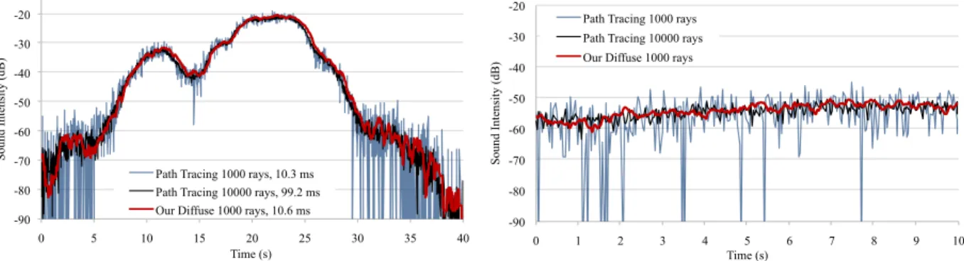
3.12 We compare the sound intensity received at the listener computed by our diffuse path cache method with that of the traditional path tracing algorithm in the office benchmark. The accuracy of our algorithm (with 1000 rays) is comparable to the path tracing algorithm (using 10000 rays) because it utilizes temporal coherence. On the other hand, path tracing with 1000 rays misses many paths and results in inaccurate
diffuse sound with significant noise and variation over time. . . 41
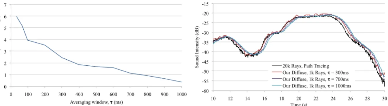
3.13 The choice of parameterτ determines how quickly the diffuse path cache will react to a change in the scene configuration. By using a longer averaging window,τ, we demonstrate that our diffuse approach converges to a small error when compared to brute-force path tracing (left). For increasingτ, we notice that there is a reaction delay of approximatelyτ versus na¨ıve path tracing when the scene is dynamic (right).
Changingτ has insignificant impact on the runtime performance of our approach. . . 42
3.14 This graph shows the sound intensity received at the listener for different values ofλ, the diffuse path cache subdivision size. Even large values ofλproduce no significant
changes in the accuracy or response time of our algorithm. . . 43
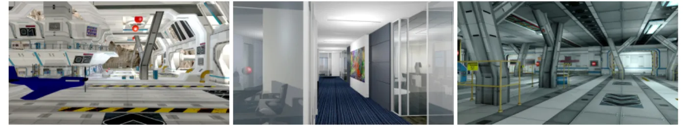
3.15 The three benchmark scenes used to evaluate our ir cache and adative IR length algorithms. The scenes have dozens of sound sources and dynamic elements (e.g. doors) that alter the sound propagation. In the hangar scene, we show a fast-moving aircraft sound source to demonstrate how the perceptual impact of our temporal
3.16 When compared to a static IR length chosen by hand for each scene, our adaptive IR length is30−60%faster for these benchmarks. The diffuse path cache of (Schissler et al., 2014) incurs significant overhead when compared to the IR cache approach. The
ray tracing time is the same for all techniques. . . 45
3.17 We compare the memory usage of our IR cache approach to the diffuse path cache of (Schissler et al., 2014) that stores individual ray paths. Our technique uses roughly 2 orders of magnitude less memory to compute sound of similar fidelity. Note that the
vertical axis has a logarithmic scale. . . 46
3.18 We compare the user evaluation results forourapproach versus thebase1andbase2
methods for 3 scenes and 2 comparison cases. For question (a), a score below 6 indicates a preference for the first method in the comparison, whereas a score above 6 indicates a preference for the second method. For question (b), the higher the score,
the more similar the audio for the two methods under comparison. . . 48
4.1 Our approach automatically estimates the acoustic materials, (a), of 3D reconstructions of real-world scenes, (b), using deep learning material classifiers applied to RGB camera images, (c). We optimize the material absorption coefficients to generate sound propagation effects that match acoustic measurements of the real-world scene using a simple microphone and speaker setup (d). The synthetic sound effects are combined
with visual renderings of captured models for multimodal augmented reality. . . 52
4.2 Our approach begins by generating a 3D reconstruction of a real-world scene from multiple camera viewpoints. Next, a visual material segmentation is performed on the camera images, producing a material classification for each triangle in the scene. Given a few acoustic measurements of the real scene, we use the visual materials as the initialization of our material optimization algorithm. The optimization step alternates between sound propagation simulation at the measurement locations and a material estimation phase until the simulation matches the measurements. The result is a 3D mesh with acoustic materials that can be used to perform plausible acoustic simulation
for augmented reality. . . 53
4.3 The results of our visual material classification algorithm for the four benchmark scenes. Colors indicate the material category that has been assigned to each triangle of the reconstructed model. The middle row shows the results of our material classification, and the bottom row shows the manually-generated ground-truth classification that are used for validation. The source and listener positions for the acoustic measurements within the real room are shown as red and blue circles, respectively. These are used to
optimize the acoustic materials present in the scenes. . . 56
4.4 An alternate view of the results of our visual material classification algorithm for the
4.5 The main results of our material optimization approach. We compare the energy-time curves and several standard acoustic parameters for the measured IRs (measured) to the results before optimization (classified) and the optimized results (optimized). We also show the results for manually-segmented materials without optimization (ground truth). The energy-time curves are presented for four octave frequency bands with center frequencies125Hz,500Hz,2000Hz, and8000Hz. The noise floor corresponds
to the signal to noise ratio of the measured IR for each frequency band. . . 65
4.6 Results of our optimization approach for alternate impulse responses. We compare the energy-time curves and several standard acoustic parameters for the measured IRs (measured) to the results before optimization (classified) and the optimized results (optimized). We also show the results for manually-segmented materials without optimization (ground truth). The energy-time curves are presented for four octave frequency bands with center frequencies125Hz,500Hz,2000Hz, and8000Hz. The noise floor corresponds to the signal to noise ratio of the measured IR for each frequency
band. . . 66
4.7 We compare the user evaluation results formeasuredcase versus theclassifiedand
optimizedcases for 4 scenes and 2 questions. For question (a), a score below 6 indicates higher audio-visual correlation for the first method in the comparison, whereas a score above 6 indicates higher audio-visual correlation for the second method. For question (b), the higher the score, the more dissimilar the audio for the two cases under
comparison. Error bars indicate the standard deviation of the responses. . . 70
5.1 Visualization to illustrate the projection of area-volumetric sound sourceSon a sphere around the listenerL. The source is approximated by many individual point sound
sources, each described by direction~xiand distanceri. . . 79
5.2 Overview of our spatial sound pipeline for area and volume sound sources. The pipeline is duplicated for each sound source in a scene. At runtime, the set of shapes for a source is first projected into the spherical harmonic basis using either the analytical formulation (spheres) or Monte Carlo ray sampling (boxes, meshes). This produces a set of basis coefficients that approximate the sound contribution from all shapes of the source. Next, HRTF filters are constructed for the left and right channels based on this projection. Finally, these filters are convolved with the anechoic input sound to
produce the final audio for that sound source. . . 81
5.3 This visualization shows the sound sources for the windmill and city scenes in red. In the windmill scene, box sound shapes are used to represent the windmill sails, spheres are used for trees, and a triangle mesh is used for the nearby river. In the city, the train and car sound sources are represented by boxes, while scrolling advertisements are
represented using meshes that correspond to the visual geometry. . . 82
5.4 The geometry of the analytical source projection for listenerLand spherical sourceS. The projection depends solely on the angleα= sin−1 Rr, whereris the distance to the sphere’s center, andRis the sphere’s radius. We choose a coordinate system for the projection with thezaxis oriented in the direction of the sphere in order to simplify
5.5 The Monte Carlo projection uses rays to sample the sound contribution from arbitrarily-shaped sources. When the listenerLis outside the bounding sphere of the sound source,S, we trace rays in the cone defined by the source’s bounding sphere. Inside the bounding sphere, rays are traced in all directions uniformly. Each ray is given a weightwithat is used to estimate the value of the projection integral. If a ray does not
hit the source, that ray haswi = 0. . . 87
5.6 The number of rays used to computed the Monte Carlo projection changes depending on the distance from the listener to the sound source’s bounding sphere. If the listener is inside the bounding sphere (left), many rays are traced in all directions. Outside the bounding sphere, the number of rays that are used for Monte Carlo integration
decreases proportional to the solid angle of the bounding sphere. . . 88
5.7 A visual representation of our spatial room impulse response construction algorithm. The IR output of sound propagation is split into partitions with sizeL, and the directiv-ity of each partition is evaluated to determine the minimum spherical harmonic (SH) order˜nfor the partition’s spatial sound. The partition’s IR is converted to the SH basis up to ordern˜, and then convolved with a SH representation of the HRTF up to ordern˜. The resulting filters for the left and right channels are added to the output SIR at the
partition’s offset in the IR. . . 90
5.8 The four benchmark scenes used to evaluate our spatial sound technique for area and volume sources. The scenes contain various large sound sources such as trains, a car,
an ocean, waterfalls, rivers, lakes, and windmills. . . 96
5.9 The performance of our approach varies with respect to the spherical harmonic order
for the four scenes. . . 98
5.10 The six benchmark scenes used to evaluate our spatial impulse response construction technique. From left to right and top to bottom: apartment, city, hangar, industrial,
subway, temple. . . 98
5.11 The performance of our spatial room impulse response construction algorithm scales quadratically with respect to the maximum spherical harmonic ordernmax. We used nmax = 4to generate the main results of our approach. The differences between the scenes are due to variation in the lengths of the impulse responses and the number of
sources. . . 100
5.12 The spherical harmonic ordern˜determined by our directivity metric for each partition varies across the impulse response length. We observe a tendency for higher SH order toward the beginning of the IR where the pressure is greater and where there are more
distinct paths with strong directivity (e.g. direct sound and early reflections). . . 101
5.13 User evaluation results for the subjective questionnaire. The comparison score is averaged over all the subjects and is plotted for each question and scene. A score of 1 represents a strong preference for the point-sampling technique and A score of 5 represents strong preference for our analytical-monte carlo technique. The horizontal dashed line presents a score of 3 indicating no preference between the two techniques. Standard deviation is represented by the error bars. The symbol * denotes significance
5.14 The results of the user evaluation of our technique. We report the average response for each question and scene, where a value of 1 indicates a strong preference for the first method (BasesorBasep), a value of 5 indicates a strong preference forourmethod, and a value of 3 indicates no preference. The error bars correspond to the standard deviation. The * symbol indicates a significance withp <0.001, while the • symbol
LIST OF ABBREVIATIONS
BRDF Bidirectional Reflection Distribution Function
C80 Clarity (ratio of early to late sound energy in decibels)
CNN Convolutional Neural Network
CPU Central Processing Unit
D50 Definition (ratio of early to late sound energy, %)
DPC Diffuse Path Cache
EDT Early Decay Time
ER Early Reflections
FIR Finite Impulse Response
FFT Fast Fourier Transform
HRTF Head-Related Transfer Function
IIR Infinite Impulse Response
IR Impulse Response
IRC Impulse Response Cache
ISM Image Source Method
LAB CIE LAB perceptual color space
LR Late Reverberation
MINC Materials in Context
RGB Red Green Blue (color space)
RGB-D Red Green Blue with Depth (color space)
RISM Ray-based Image Source Method
RT60 Reverberation Time (the time for pressure to decay by 60 dB)
SH Spherical Harmonics
SIFT Scale Invariant Feature Transform
SNR Signal to Noise Ratio
SPC Specular Path Cache
SPL Sound Pressure Level
LIST OF SYMBOLS
Math Functions:
Ylm(~x) Spherical harmonic (SH) basis functions as a function of direction~x
n Spherical harmonic order
δ(x) Dirac delta function
Counts, Objects:
Ni Number of sound propagation paths
Nr Number of primary rays emitted from source or listener NT Number of triangles in the environment
NS Number of sound sources in the environment NL Number of listeners in the environment Tj Thejth triangle in the environment Sk Thekth sound source in the environment Ll Thelth listener in the environment
d Acoustic interaction order
dmax Maximum acoustic interaction order
Sound Attributes:
r Sound propagation path length in meters
t Time, in seconds
ω Frequency
¯
ω Frequency band centered atω
ti Delay time for sound propagation pathi ~
xi Incoming world-space sound propagation direction at the listener for pathi X(~x) Distribution of incoming sound intensity at the listener for frequency bandω¯ Xlmω¯ Spherical harmonic coefficients for distribution of intensity for bandω¯ Iiω¯ Sound intensity for propagation pathiand frequency bandω¯
c Speed of sound in propagation medium
z0 Characteristic specific acoustic impedance of the propagation medium
P Sound power, in watts
Tq(ω) Absolute threshold of human hearing as a function of frequencyω
Temporal Coherence:
K Specular path identifier, sequence of triangle reflections
λ Triangle subdivision patch size
(ζ, ξ) Triangle subdivision patch location identifier
~
q Ray-triangle intersection point
(γ0, γ1, γ2) Baycentric coordinates of~q
η Number of rays that reach the listener for a diffuse reflection path cache entry
µ Number of rays emitted from the source while diffuse cache entry was valid
τ Temporal coherence smoothing time constant, in seconds
α Exponential smoothing factor determined fromτ.
Material Optimization:
R Sound intensity reflection coefficient
α Sound pressure absorption coefficient for random sound incidence
b Impulse response intensity histogram bin
m Material patch
Wω¯ Acoustic optimization weight matrix for frequency bandω¯ wωbm¯ Entry of weight matrix corresponding to IR binband materialm pS(t) Optimization simulated pressure impulse response
pT(t) Optimization target pressure impulse response
IωS¯(t) Intensity-time curve for optimization simulated IR
IωT¯(t) Intensity-time curve for optimization target IR
IωbS¯ Intensity-time histogram for optimization simulated IR
IωbT¯ Intensity-time histogram for optimization target IR
Sound Rendering, Spatial Sound:
p(t) Pressure impulse response as a function of time
pL(t) Pressure impulse response for the left ear pR(t) Pressure impulse response for the right ear s(t) Anechoic sound source audio in units of pascals
qL(t) Sound source audio received by listener’s left ear qR(t) Sound source audio received by listener’s right ear
H(~x, t) Head-related transfer function as a function of direction~xand timet hlm(t) Head-related transfer function in the SH domain as a function of timet hlm(ω) Head-related transfer function in the SH domain as a function of frequencyω
CHAPTER 1: INTRODUCTION
One of the most important human senses is our sense of hearing, the ability to perceive sound. Sound
is a pressure wave produced by the vibration of an acoustic medium such as air or water. As humans, we
can hear sound waves with frequencies between20Hz and20,000Hz. Sound below this frequency range
is calledinfrasound, while sound above this frequency range is calledultrasound. Hearing is the second
most important sense that we use to interact with the environment (Blauert, 1997). Soundhas been a primary
medium for the development of language, music, and possibly human intelligence. In the present day, sound
remains an important part of everyday life as a vehicle for communication, education, and entertainment.
Sound propagation is the process by which pressure waves are emitted from a source into the propagation
medium, transmitted and reflected through the environment, and eventually heard by a listener. When sound
is produced, it can have various interactions with the environment. These include reflection, scattering,
diffraction, air absorption, and refraction. During sound propagation, sound is delayed and attenuated in
ways that provide a listener information about the environment and sound sources. The effects of sound
propagation are responsible for familiar phenomena like echoes, reverberation, and Doppler shifting, as well
as the subjective audible differences between environments like a gymnasium, office, forest, or cathedral.
1.1 Sound Propagation
Sound is a wave consisting of alternating regions of high and low pressure in a sound propagation medium.
The distance between successive pressure highs or lows is the wavelength. The wavelength for sound at
audible frequencies in air ranges from about1.7cm to over17m. Sound is emitted from a source when small
surface vibrations cause the surrounding medium to vibrate in the form of pressure waves. These waves then
propagate from the source at the speed of sound,c≈343m/s in air at room temperature. If the sound source is omnidirectional, the same pressure waves are radiated in all directions. However, most sound sources
including the human voice are highly directional and radiate sound in a frequency and direction-dependent
After sound is emitted from the source, it propagates through the environment. When sound interacts
with an object in the environment, it may be reflected, scattered, attenuated, diffracted, and transmitted
according to the material of the object. The acoustic material properties depend on the wavelength of sound
and are impacted by characteristics such as surface roughness, density, and the presence of hidden resonant
cavities. The materials in an environment have a strong influence on the sound heard by the listener.
When a sound wave is reflected from a flat rigid surface much larger than the wavelength, it is reflected in
a mirror-like or specular manner. With specular reflections, the incoming wavefront is deflected in a direction
that has the same angle relative to the surface normal. If the surface of an object has bumps or roughness
that is of the same scale as the wavelength, the incident sound wave may be scattered rather than perfectly
reflected. This kind of reflection is called a diffuse reflection. A perfectly diffuse surface would scatter the
same amount of sound in all directions in the surface hemisphere. Many acoustic materials exhibit a mixture
of specular and diffuse reflection at different frequencies. Reflections are responsible for producing echoes,
delayed copies of the original sound. The first few reflections of sound from the environment are called the
early reflections. When many successive high-order reflections occur, the sound becomes increasingly diffuse
and smoothly-decayingreverberationis produced.
When the wavelength of sound is larger than features in the environment, diffraction effects become
significant. Diffraction is a wave phenomenon where sound is scattered by features that are similar in scale to
the wavelength. Diffraction is most evident at lower frequencies and is responsible for sound bending around
corners or objects, as well as the scattering of diffuse reflections. Diffraction can enable a listener to hear a
sound source even though the source may be visually occluded.
Sound that interacts with a surface in the environment may also have some of its energy transmitted into
the material behind the surface. This process is known as sound transmission. During transmission, the sound
wave undergoes a change of medium (e.g. from air to water), and this causes attenuation that varies with the
sound frequency. Transmission allows sound to travel through walls, windows, and other non-rigid materials,
then possibly exit back into the air. Transmission effects are an important consideration for noise control
applications where it is useful to limit the amount of outside noise that enters a quiet building.
If sound changes medium during its propagation, it can also be refracted. Refraction is a bending of the
pressure wave that occurs when the speed of sound changes. Refraction can occur in the atmosphere due to
body of water at night. The water cools the air near the surface, decreasing the speed of sound and causing
sound waves emitted upward from the source to bend down toward the ground on the other side of the water.
If sources, listeners, or objects in the environment move quickly, then Doppler shifting may occur. The
Doppler effect is a phenomenon where the frequency of sound is changed due to compression or expansion
of pressure waves caused by the moving objects. This effect is most commonly encountered when a vehicle
drives past a stationary listener. As the vehicle approaches, its sound is raised in frequency because pressure
waves are compressed ahead of the vehicle. Then, as the vehicle passes the listener the pitch of the vehicle’s
sound decreases as the pressure waves emitted from behind are expanded. The Doppler effect is more
noticeable when sound sources move more quickly, i.e. a race car moving at 200 km/h will shift the frequency
more than a slow-moving truck.
When sound arrives at the listener’s position, it is affected by the listener’s head and torso before it arrives
in the listener’s ear canals. This phenomenon, commonly referred to asspatial sound, produces variation in
the level and delay of sound for different frequencies and directions. The sound heard by the left and right
ears tends to be different, and the brain exploits those differences to perceive spatial information about the
environment, including the location of the sound sources.
In comparison to visible light, a form of electromagnetic radiation, sound is characterized by its wide
frequency range and long wavelength that is of the same scale as everyday objects. Therefore, diffraction
effects are much more prominent for sound than light, which has too small a wavelength to diffract at human
scales. Another difference between sound and light is that the phase and time delay of sound is perceptually
important, whereas light travels so quickly that most phase differences are imperceptible to the human
eye. The inclusion of phase and diffraction effects causes some significant differences between rendering
algorithms designed for graphics and sound.
1.2 Motivation
Sound propagation has a wide variety of applications in diverse areas including the entertainment industry,
architecture, engineering, noise control and teleconferencing.
Virtual reality (VR) has seen renewed interest in recent years as commodity head-mounted displays have
the users’s sense of presence and immersion in the virtual environment (Hendrix and Barfield, 1996). VR
requires high-fidelity sound propagation to be rendered with low latency.
A related application to VR is training simulations. Training simulations are frequently used by the
military and emergency services to prepare trainees for dangerous situations in a safe environment. In these
simulations it is critical to generate audio that has realistic sound propagation in order to produce the most
faithful simulation.
Video games are another area where sound propagation can significantly improve the experience. Like
with VR, audio must be generated for the virtual environments found in games. While games may not always
focus on generating the most realistic sonic environment, sound propagation can nevertheless be used to
enhance atmosphere, immersion, and gameplay. For example, sound propagation can allow players in a
multiplayer game to locate hidden adversaries by the sound of their footsteps.
In augmented reality (AR), sound propagation can be used to generate audio for virtual objects that are
placed in real environments. The augmented audio can improve the users’s sense that the virtual object exists
physically if it is rendered with the sound propagation effects of the real room.
Teleconferencing is another application of sound propagation, where users communicate remotely using
an audiovisual connection. Sound propagation can be used to render the remote audio in a way that makes
the remote user seem as if they were in the local room.
In the movie, television, and music industries, reverberation is frequently added to sound recordings
to enhance the plausibility. Sound propagation can reduce the amount of work involved for audio mixing
engineers when trying to replicate a particular sonic environment using digital filters.
Another major application of sound propagation is in architectural acoustics, where it may be important
to predict how a particular room or CAD model of an architectural space will sound before it is constructed.
This is especially important for the design of concert halls and auditoriums that require certain acoustic
characteristics. A significant focus of architectural acoustics is determining which materials (e.g. acoustic
panels) should be used that produce the best sound for a particular application. Sound propagation also has
applications in interactive walkthroughs, where it is useful in generating virtual walkthroughs of real spaces.
Simulation of realistic sound in walkthroughs can enable a potential real estate buyer to avoid spaces that
In city planning, it is important to simulate sound propagation so that noise can be effectively controlled
in sensitive locations such as schools, hospitals, and residential areas. Sound propagation can be used in the
placement of noise barriers in relation to loud places like airports and factories.
Within engineering applications, sound propagation can be used in the design process to achieve desired
levels of acoustic performance, such as to reduce the interior noise of passenger cars and aircraft cabins or to
reduce the exterior noise pollution generated by combustion engines.
1.3 Challenges
Due to the complexity of sound propagation phenomena, high-quality interactive simulation of sound
propagation in dynamic environments remains a challenging problem. To achieve interactive performance,
the simulation must be updated with a latency of less than about100ms (Lindau, 2009). Many previous
approaches have been proposed that simulate sound propagation phenomena using geometric techniques.
The RAVEN system (Lentz et al., 2007) is a state of the art interactive geometric sound propagation system.
It is mainly designed for indoor scenes and supports specular reflections, diffuse reflections, diffraction, and
spatial sound. However, it takes a few seconds to compute a single simulation update, and therefore is not that
suitable for highly interactive applications like virtual reality. The RESound system (Taylor et al., 2009) takes
about250−500ms to model 3rd-order diffuse and specular reflections using ray and frustum tracing. More recent ray tracing methods have improved on these results by using guided ray tracing (Taylor et al., 2012),
and can compute 3rd-order reflections and 1st-order diffraction in about93ms for a few sources in scenes
typical of interactive games. Other approximate methods have been proposed that estimate the reverberation
in environments using heuristic algorithms (Antani and Manocha, 2013). These techniques can update the
simulation in about10ms, however they introduce numerous approximations and simplifications that can
impact the plausibility of the results. In general, previous approaches are able to simulate a few orders
of reflection and 1st-order diffraction for a few sound sources in a hundred milliseconds. More complex
high-order reflections or diffraction can take a second or more to compute. As a result, there are still many
challenges that must be addressed to enable low-latency interactive sound propagation:
Interactive performance:One of the largest problems faced by previous sound propagation techniques is
for computing sound propagation are based on geometric acoustics and ray tracing. However, the quality
and performance of ray tracing depends strongly on the number of rays traced. Current sound ray tracing
algorithms require a large number of rays to produce noise-free results. Roughly 10,000 - 50,000 rays must
be emitted from each source (Lentz et al., 2007; Taylor et al., 2012), and those rays must be propagated
for about 200 bounces to simulate late reverberation. This leads to about 2-10 million rays per source per
simulation update. Recent advancements in ray tracing for graphics have enabled tens of millions of rays to
be traced per second on the CPU (Wald et al., 2014). However, the performance on complex environments
with many sound sources is not sufficient, since it may take hundreds of milliseconds for each sound source.
As a result, it is difficult to apply ray tracing approaches directly to interactive applications due to the large
update latency.
Acoustic material acquisition: Another significant challenge in computing sound propagation for virtual
and augmented reality environments is that accurate acoustic material properties are necessary to compute
plausible sound, yet are difficult to acquire. Some previous approaches manually assign a material for every
surface from a database of measured material data. However, this process is time consuming and requires
expert knowledge of how sound interacts with materials to produce accurate results. Automatic approaches
have also been proposed that use optimization algorithms to assign materials properties (Monks et al., 2000;
Christensen et al., 2014; Saksela et al., 2015), however they have very slow convergence or are limited
to virtual scenes. Furthermore, the resulting simulations may not match known acoustic characteristics of
real-world scenes due to inconsistencies between the measured data and actual scene materials. Mismatch
between the sound simulation and real world can interfere with the subjective presence and realism of virtual
sound sources placed within real-world environments.
Spatial sound: A drawback of current techniques for modeling spatial sound is that they focus on point
sound sources and are inefficient for large sources that occupy an area or volume. As a result, current spatial
sound techniques are not interactive when handling sources such as oceans, rivers and lakes. An additional
challenge is that spatial sound cannot be rendered interactively for sound propagation effects. With sound
propagation, sound arrives from various directions at different times. This greatly increases the complexity
latency is experienced by the user as a delay or lag in the sound. The perception of latency is strongest when
the listener is quickly rotating their head. This latency strongly detracts from the plausibility and interactivity
of dynamic scenes.
1.4 Thesis Statement
Sound propagation can be efficiently rendered for interactive, dynamic, multi-source environments
through the use of temporal coherence, automatic material classification, and low-latency spatial sound.
In this dissertation, we describe a collection of novel techniques that enable simulation and rendering
of sound propagation in large, complex, multi-source environments at interactive rates. Our first goal
is to improve the performance problems of existing interactive sound propagation algorithms by reusing
computations executed on previous simulation time steps. Next, we demonstrate how acoustic materials
can be automatically determined using a combination of visual and audio measurements of real-world
environments. Finally, we propose spatial sound techniques that enable high-quality, low-latency directional
audio to be efficiently computed for sound propagation. We have evaluated the impact of these improvements
on a variety of benchmarks and shown that our approach enables efficient interactive simulation of sound
propagation in complex, dynamic environments.
1.5 Main Results
In this dissertation, we present three approaches for interactive sound propagation in dynamic scenes.
First we discuss how temporal coherence can be used to improve the interactive performance of sound
propagation. Next, we propose an automatic acoustic material classification and optimization algorithm that
is used to estimate the material properties that are present in real environments. Finally, we show how spatial
sound can be efficiently rendered for sound propagation with low latency. Figure 1.1 illustrates how these
ideas can be integrated into a complete sound propagation and rendering pipeline.
1.5.1 Temporal Coherence for Sound Propagation
While many previous techniques have been proposed for interactive sound propagation using geometric
Paths
IRs
Spatial Sound Acoustic
Materials Classification
Temporal Coherence
Optimization RGB
Images
Measured IRs
Material Estimation
Sound Propagation
Cache
Paths IRs IRs,
IR length
Paths
Spatial Sound Rendering
HRTF
Spatial IRs
Source Audio
Figure 1.1: A high-level overview of our material estimation, sound propagation, and spatial sound rendering pipeline. We use RGB images of the environment along with measured impulse responses to automatically estimate the acoustic materials. Then, we use sound propagation and temporal coherence techniques to efficiently compute interactive sound propagation. The resulting propagation paths and impulse responses are used by the sound rendering module to compute the final audio using convolution with a spatial impulse response.
simulation update. As a result, previous methods are limited to either static precomputed scenes or only a few
sound sources.
We propose a novel approach that reduces the work that must be performed on each time step by using
sound propagation results from previous time steps. This cached information, including propagation paths
and impulse responses, is stored in persistent data structures and is used to improve the simulation quality
and reduce sampling noise caused by tracing too few rays. Our approach is based on the assumption that
the sound field at the listener’s position does not change quickly over time in most situations, e.g. there is
temporal coherence. The main contributions of this technique include:
1. Specular path cache:A cache of specular early reflection paths from previous frames is maintained
in order to reduce the computation needed to find specular paths on current and future frames.
2. Diffuse path cache:Diffuse early reflection paths are grouped together based on a surface subdivision
and cached over several frames. A moving average filter uses paths from previous and current frames
to estimate a diffuse sound field with less sampling noise.
3. Impulse response cache:A cache of the impulse response between each source and listener from the
previous frame is used to improve the quality of high-order diffuse ray tracing with low computational
and memory overhead.
4. Adaptive impulse response length: The listener’s threshold of hearing is applied to the previous
This technique has been tested on a variety of complex indoor and outdoor scenes, and has been shown
to reduce the computation required, in terms of the number of rays, for interactive sound propagation by over
an order of magnitude as compared to previous approaches based on ray tracing.
1.5.2 Acoustic Material Classification and Optimization
A significant issue with the extension of sound propagation to augmented reality and architectural
applications is that the material properties of the real environment can be difficult to accurately acquire.
Previous techniques have relied on manual assignment of materials, but this is time-consuming and may not
always produce accurate results.
We propose a new automatic approach for estimation of acoustic materials in real environments. Audio
and visual captures of the environment are used within a two-step process that involves using visual
infor-mation to classify the material categories that are present, then optimizing those materials until the acoustic
simulation in the virtual room matches the audio in the real room. The main contributions are summarized as
follows:
1. Material classification:The visual appearance of the scene is captured in many color images which
are the input to a convolutional neural network (CNN). The CNN has been trained to recognize common
real-world material categories at each point in a color image. The material predictions are projected
from each image into the scene and are then used to determine the final material categories for every
surface primitive.
2. Material optimization:Given measured impulse responses from the real scene, an iterative
optimiza-tion algorithm is used to improve the accuracy of the material estimates. On each iteraoptimiza-tion, a simulaoptimiza-tion
is used to gather information about sound transport within the scene. Then, a least-squares formulation
solves for the material absorption values that best match the measured impulse responses.
This approach has been applied to several real-world environments and its effectiveness has been both
quantitatively and subjectively evaluated. With automatic material acquisition, realistic sound effects can be
1.5.3 Low-Latency Spatial Sound for Sound Propagation
The computation of accurate spatial sound is a significant bottleneck for interactive sound rendering
when applied to the complexity of realistic sound propagation. In this case, sound arrives at the listener
from many directions at different delay times, and each sound arrival must be auralized with the directional
filtering of the listener’s head geometry.
We present a technique for efficient rendering of spatial sound with low latency using the spherical
harmonic (SH) basis functions. Our approach represents the sound field at the listener’s position in the
SH domain, and then takes advantage of SH orthonormality to efficiently construct spatial sound filters for
area and volume sources as well as sound propagation impulse responses. The primary contributions of our
technique include:
1. Area and volume sources:The projection of sound pressure arriving at the listener’s position from
all directions is used to compute the spatial sound filter for sources that emit sound over a large area or
volume.
2. Spatial impulse response construction: A perceptual metric is used to adaptively determine the
spherical harmonic order to use for each partition of a sound propagation impulse response.
We have implemented this approach within the Unity™game engine and evaluated the performance and
subjective quality of the results with user studies. A speedup of at least an order of magnitude is achieved in
each case over the previous technique, enabling high-quality spatial sound to be computed with low latency
for interactive sound propagation.
1.6 Organization
The remainder of the dissertation is organized according to the following structure:
• InChapter 2, we introduce relevant background and previous work on sound propagation, acoustic
materials, audio rendering, and spatial sound.
• Chapter 3describes how temporal coherence can be used to improve the performance of interactive
• InChapter 4, a technique for automatic acquisition of acoustic materials in real world scenes is
presented, along with comparisons to real-world measurements.
• Chapter 5introduces techniques for efficiently rendering spatial sound filters for area and volume
sound sources, as well as a method for perceptual spatial impulse response construction.
CHAPTER 2: BACKGROUND
2.1 Sound Propagation
When sound propagation is computed for a virtual environment, the goal is to determine the how the
sound emitted by each source is affected by the environment before it is received at the listener. This can be
modeled as a filter whose impulse response (IR) specifies how sound is delayed and attenuated due to sound
propagation. Sound propagation algorithms can be divided into two main classes: those that numerically
solve the acoustic wave equation, the so-calledwave-basedmethods, and those that use geometric algorithms
to approximate sound propagation phenomena, thegeometricmethods.
2.1.1 Wave-based Sound Propagation
Wave-based sound propagation algorithms are both the most accurate and computationally expensive
methods. Time-domain solvers divide the simulation domain into cubic or rectangular volume partitions
that have an analytical solution to the wave equation, then compute how sound waves propagate within and
between the partitions. These include Finite Difference Time Domain (FDTD) (Savioja, 2010) and Adaptive
Rectangular Decomposition (ARD) (Raghuvanshi et al., 2009). Other approaches such as the Boundary
Element Method (BEM) solve the wave equation in frequency domain given the boundary conditions on
every surface in the scene (Ciskowski and Brebbia, 1991). While wave-based methods are widely used in
scientific and engineering applications, the computation time and memory required scales very poorly with
the maximum frequency and size of the simulation domain. Therefore they are usually limited to offline
simulation. On the other hand, precomputation and compression approaches have been proposed that enable
interactive wave-based sound propagation with a dynamic source and listener in static scenes (Raghuvanshi
2.1.2 Geometric Sound Propagation
Geometric sound propagation techniques are based on the simplifying assumption that the surface
primitives in the environment are much larger than the wavelength of sound. As a result they can more easily
simulate dynamic scenes at interactive rates. While this assumption is valid for high frequencies, geometric
algorithms are inherently less accurate at low frequencies where wave phenomena like diffraction must be
modeled explicitly.
2.1.2.1 Specular Reflections
Many algorithms have been proposed for the computation of specular reflections. In the image source
method (Allen and Berkley, 1979; Borish, 1984), point sound sources are recursively reflected over every
surface primitive to form a tree of possible reflection paths, then the valid unoccluded paths are determined
by tracing rays from the listener position back to the source. The complexity of the basic image source
method can be improved by using ray tracing to sample the most likely reflection paths (Ondet and Barbry,
1989). In beam tracing (Funkhouser et al., 1998) and frustum tracing (Chandak et al., 2008), rectangular
beams or frusta are propagated from the source and recursively reflected to build a tree of possible paths
that are validated using ray tracing. A significant drawback of these techniques is that they are limited to
specular reflections and cannot model the later parts of the impulse response where the sound becomes more
diffuse (Lentz et al., 2007).
2.1.2.2 Diffuse Reflections
The most common techniques for computing diffuse reflections are based on Monte Carlo path tracing,
a probabilistic technique for solving complex integral equations (Krokstad et al., 1968; Vorl¨ander, 1989;
Embrechts, 2000). In path tracing, rays that each carry a fraction of the total sound energy are randomly
emitted from the source. The rays are reflected throughout the environment until an intersection with
the listener is detected, thereby generating a sound propagation path that is accumulated to the impulse
response. The convergence of path tracing can be improved by direct sound sampling techniques such as
diffuse rain(Schr¨oder et al., 2007). Path tracing is often computed in separate frequency bands to model
frequency-dependent scattering and attenuation. Radiosity may also be used for the computation of diffuse
2.1.2.3 Diffraction Modeling
Diffraction can be approximated within the geometric sound propagation framework using specialized
diffraction techniques. The simplest methods are based on single-point diffraction over infinite edges and
include the Geometric Theory of Diffraction (GTD) (Keller, 1962) and the Uniform Theory of Diffraction
(UTD) (Kouyoumjian and Pathak, 1974). While computationally efficient to evaluate, these techniques
become much less accurate when applied to complex environments with many small edges. The more
expensive Biot-Tolstoy-Medwin (BTM) method (Svensson et al., 1999) instead computes a line integral over
diffraction edges and can handle edges of any length with higher accuracy. Another approach for geometric
diffraction modeling is based on the Heisenberg uncertainty principle (Stephenson, 2010) and it can be easily
integrated within a path tracing framework.
2.2 Acoustic Materials
The acoustic materials that are present in an environment have a strong influence on the resulting sound
propagation. One of the most important material properties is the absorption coefficient,α ∈ [0,1].The absorption coefficient describes the fraction of incident sound pressure that is absorbed when a sound wave is
reflected by a surface.αis usually a function of both frequency and the angle between the incident direction and the surface normal. It can be measured according to ISO 354 (ISO, 2003) where a sheet of the material
to be measured is a placed in a reverberation chamber, then the absorption is derived from the difference in
reverb time using the Sabine equation (Sabine, 1922).
The scattering behavior of a material is most commonly described by the frequency-dependent scattering
coefficients ∈ [0,1]. srepresents the fraction of incident sound that is reflected diffusely (e.g. with a Lambertian distribution) and is correlated to the roughness of the surface (Christensen and Rindel, 2005).
More complex scattering can be represented using bidirectional reflection distribution functions (BRDFs)
that describe the outgoing energy distribution for a given incident direction and frequency (M¨uckl and
Dachsbacher, 2014), though acoustic BRDFs are difficult to measure in practice.
Many approaches have been proposed that determine the acoustic materials of an environment using
optimization techniques. Monks et al. (Monks et al., 2000) present a method for optimizing the placement
rials so that the resulting simulations match real-world measurements, but the rate of convergence is very
slow (Christensen et al., 2014). (Saksela et al., 2015) use least squares regression in combination with beam
tracing to optimize surface absorption coefficients for virtual rooms. The impedance of acoustic materials in
a real scene can be estimated for individual frequencies using acoustic measurements of pure tones and the
inverse boundary element method (Nava, 2006).
2.3 Sound Rendering
The earliest techniques for rendering sound propagation are based on artificial reverberators, recursive
feedback-delay filters that mimic the rate of decay of natural late reverberation in indoor rooms (Schroeder,
1961). The realism of artificial reverberators can be improved by rendering early reflections using additional
delay taps (Gardner, 2002), or by simulating frequency-dependent sound absorption using a low pass filter
in the feedback loop (Schroeder, 1961). The reverberation parameters can also be initialized by analysis
of the impulse response between the source and listener (Taylor et al., 2009). While these techniques are
computationally efficient, they are unable to simulate time-varying directional reverberation or outdoor
environments.
More sophisticated sound rendering methods use convolution of the source audio with the impulse
response to generate realistic sound. Na¨ıve time-domain convolution is expensive for long impulse responses,
but IR partitioning schemes and frequency domain convolution can be used to improve both the latency and
performance (Gardner, 1994). Convolution can reproduce most sound propagation phenomena except for
Doppler shifting.
To render the pitch shifting inherent to the Doppler effect, fractional delay interpolation can be used
on direct and early reflection paths. However, it is too expensive to render Doppler shifting for all sound
propagation paths for interactive applications. Delay interpolation involves reading from a circular delay
buffer at a rate that depends on the relative velocity between the source and listener along the propagation
path, thereby either compressing or expanding the sound waves along the time axis (Strauss, 1998).
2.3.1 Spatial Sound
A perceptually important aspect of sound rendering is the generation of spatial sound such that the
panning (VBAP) (Pulkki, 1997), where the vector to the sound source is used to compute the amplitude
of each channel in a 3D array of loudspeakers. While computationally efficient, VBAP does not model
phenomena like the different times of sound arrival at each ear or frequency-dependent scattering from the
head and torso. The directional behavior of the listener is best described by the head-related transfer function
(HRTF). The HRTF is a function of either time or frequency on the spherical domain. By interpolating an
HRTF measured for a listener and convolving the interpolated HRTF filter with the audio for the source,
the listener is given the impression that the source is in a particular direction. To generate HRTF-based
spatial sound for sound propagation, the HRTF is convolved with the impulse response to generate a spatial
impulse response (SIR), then the SIR is convolved with the source audio. Due to the expense of convolving
the HRTF with the IR, current methods either only apply the HRTF to important direct and early reflection
paths, or cluster paths based on direction to reduce the number of HRTF interpolations (Lentz et al., 2007).
However these methods introduce error and are still too slow for dynamic interactive simulations. As a result,
CHAPTER 3: TEMPORAL COHERENCE FOR SOUND PROPAGATION1
3.1 Introduction
In simulations of interactive sound propagation, it is common to update the simulation state in a series
of discrete time steps that are referred to asframes. On each frame, a new collection of impulse responses
between each source and listener are computed and used for auralization. While traditional geometric
acoustics algorithms based on ray tracing are among the fastest ways to compute these impulse responses, the
quality and performance of ray tracing depends strongly on the number of rays traced and how many orders of
reflection are computed. Sound propagation approaches based on Monte Carlo path tracing involve generating
many random rays to sample sound propagation paths within the scene. Those paths are then used to estimate
the sound intensity received by the listener. The more rays that are traced, the more accurate this estimation
will be, but at increased computational expense. If not enough rays are traced, the space of propagation paths
will not be effectively sampled, resulting in noise in the computed impulse response. This noise is most
audible in interactive sound propagation where the impulse response and rendered audio changes noticeably
each time it is updated. Rendering directional spatial sound exacerbates this effect, producing sound that
seems to move around the listener as different propagation paths are detected on each simulation update.
As a result, the number of rays that are required for artifact-free audio can be very large. In addition, it
is not knowna priorihow many secondary ray bounces should be computed for each primary ray, as this
depends on factors such as the scene geometry, the position and loudness of the source, and the acoustic
materials present in the scene. If not enough bounces are computed, it can truncate the end of the impulse
response, while if too many bounces are computed, the unnecessary computation may be wasted. If these ray
parameters are not carefully chosen, it can either negatively affect the sound quality, or lead to non-interactive
performance for complex scenes.
In this chapter, we present techniques that are based on the observation that the sound at the listener does
not change very quickly in most scenes, i.e. there istemporal coherence. Our algorithms use information
1
computed on previous simulation frames, such as sound propagation paths and impulse responses, to reduce
the number of rays and ray bounces that are needed on each frame for sufficient sound quality. Similar ideas
have been proposed in the graphics literature in order to reuse shading results from previous frames or to
incorporate temporal antialiasing (Scherzer et al., 2011). First, we focus on how temporal coherence can
be utilized in the computation of specular early reflections (Section 3.2.1). A data structure known as the
specular path cacheis used to cache specular reflection paths from previous frames, thereby reducing the
cost involved in finding paths on future frames, allowing fewer rays to be traced, and improving performance.
Next, we propose an approach for diffuse reflections that uses adiffuse path cacheto utilize ray tracing from
previous frames (Section 3.2.2). A moving average filters the sound intensity for each diffuse reflection
path over many frames. This increases the accuracy of Monte Carlo path tracing by taking more rays into
account. In Section 3.2.3, we present another temporal coherence technique that uses a cached copy of the
previous impulse response, theimpulse response cache, in order to filter the path tracing IR using exponential
smoothing (Brown, 1956). This approach is notable in that it can be implemented very efficiently and enables
fast computation of high-order reflections. Finally, we describe a method for adaptively determining the
length of the impulse response using the IR from the previous frame and a perceptually-based threshold
(Section 3.2.4). The IR length is used to determine how many secondary ray bounces should be computed on
the next frame without truncating the IR or performing unnecessary computation.
We have evaluated the subjective and performance impacts of these approaches on a variety of complex
scenes and demonstrate that temporal coherence can enable dynamic sound propagation effects to be computed
at interactive rates.
3.2 Temporal Coherence for Sound Propagation
In this section we describe temporal coherence techniques that can be used to improve the quality and
performance of interactive sound propagation. An overview of our approach is shown in Figure 3.1. We
utilize several data structures to cache information that improves the results for various components of sound
propagation. These include thespecular path cache(Section 3.2.1), thediffuse path cache(Section 3.2.2),
and theimpulse response cache(Section 3.2.3). Using these ideas, we obtain significant benefit over previous
Specular Cache Diffuse Cache IR Cache Sound Propagation with Temporal Coherence
Ray-based Image
Source Method Monte Carlo Path Tracing
Specular ER
paths Diffuse Paths
IRs, IR length
Paths
IRs Scene
Figure 3.1: A high-level overview of our sound propagation technique that uses temporal coherence. We cache specular reflection paths, diffuse reflection paths and impulse responses in order to improve the sound quality for interactive applications.
3.2.1 Specular Path Cache
The early reflections (ER) are a perceptually important component of sound propagation that correspond
to the first several orders of reflection and that consist of mostly specular sound energy (Lentz et al., 2007). A
widely-used algorithm for computation of specular reflections is the image source method (Allen and Berkley,
1979; Borish, 1984). The image source method as originally described has a complexity ofO(Ndmax
T ), where NT is the number of triangles in the environment, anddmaxis the maximum reflection order. As a result, various acceleration techniques have been proposed such as beam tracing (Funkhouser et al., 1998) and
frustum tracing (Chandak et al., 2008) that use volume intersection queries to reduce the number of possible
reflection paths that must be checked for validity. The ray-based image source method (RISM) (Ondet and
Barbry, 1989) instead uses stochastic ray tracing to efficiently sample possible paths. Unlike beam and
frustum tracing, the performance and quality of the ray-based image source method is largely dependent on
the number of primary rays that are emitted from the source or listener. If not enough rays are traced, some
propagation paths may not be explored, and if different random rays are traced on each frame it can introduce
unnatural variation in the sound from frame to frame. However, if too many rays are traced, computation is
wasted on redundant path validation.
In this section we propose an algorithm that is an extension to the ray-based image source method and
utilizes temporal coherence to reduce the number of rays traced while maintaining similar sound quality. A
primary component of our algorithm is a data structure called thespecular path cache(SPC). The specular
path cache is used within the RISM to reduce the number of rays needed and to reduce unnatural variation