THREE STUDIES ON THE DETERMINANTS AND CONSEQUENCES OF POVERTY
Colin Scott Campbell
A dissertation submitted to the faculty at the University of North Carolina at Chapel Hill in partial fulfillment of the requirements for the degree of Doctor in Philosophy in the Department
of Sociology.
Chapel Hill 2014
Approved by: Arne L. Kalleberg Guang Guo
Kathleen Mullan Harris Ted Mouw
ABSTRACT
Colin Campbell: Three Studies on the Determinants and Consequences of Poverty (Under the direction of Arne L. Kalleberg)
In this dissertation I consider the effect of dropping out of high school on poverty and welfare receipt, the effect of sibship size on cognitive ability and early educational achievement, and the determinants of support for government involvement in lessening poverty. Using a variety of multivariate methods and data sources, (1) I find that dropping out of high school has an independent effect on poverty and welfare receipt net of unobserved background
ACKNOWLEDGEMENTS
I am deeply indebted to my dissertation committee. Arne Kalleberg, my advisor and committee chair, provided invaluable advice, helped make sure I was always able to meet deadlines, and steered me away from more than a few bad dissertation topics. Ted Mouw took my ideas and made them better. The other members of my committee, Guang Guo, Kathleen Mullan Harris, and François Nielsen, read drafts, offered guidance, and greatly improved my dissertation.
I am also grateful for the help that I received from my friends and colleagues.
Conversations with Shawn Bauldry, JD Daw, Jason Freeman, Michael Gaddis, Jessica Pearlman, Ashton Verdery, Brandon Wagner, and Tiantian Yang shaped my understanding of what I wanted to accomplish in my dissertation. I am especially thankful for the conceptual and methodological assistance that I received from Jessica Pearlman. I am also grateful for the personal support that I received from my parents, brother and sister, friends, and Heather.
Lastly, I would like to acknowledge the financial and professional development support that I received from the Graduate School at the University of North Carolina at Chapel Hill in the form of a dissertation completion fellowship in the Royster Society of Fellows.
TABLE OF CONTENTS
LIST OF TABLES………...viii
LIST OF FIGURES………...x
CHAPTER 1: INTRODUCTION AND OVERVIEW Section 1.1: Overview of Dissertation……….5
High School Dropouts, Poverty, and Welfare……….5
Sibship Size, Cognitive Ability, and Early Educational Achievement…………....8
Economic Hardship and Beliefs about Government Spending on Poverty……...11
References………..15
CHAPTER 2: THE SOCIOECONOMIC CONSEQUENCES OF DROPPING OUT: EVIDENCE FROM TWO COHORTS OF SIBLINGS………16
Introduction………...16
Background………...19
Data and Measures………25
Analytic Strategy………...29
Findings………33
Discussion………52
References………56
CHAPTER 3: SIBSHIP SIZE, COGNITIVE DEVELOPMENT, AND EARLY EDUCATIONAL ACHIEVEMENT IN LOW-INCOME HOUSEHOLDS………61
Background………...62
Data and Measures………..68
Analytic Strategy………...72
Findings………...80
Discussion………...91
References………...94
CHAPTER 4: THE FORMATIVE YEARS, ECONOMIC HARDSHIP, AND BELIEFS ABOUT THE GOVERNMENT’S ROLE IN LESSENING POVERTY………101
Introduction……….101
Background……….103
Data, Measures, and Methods……….108
Findings………...114
Discussion………....126
LIST OF TABLES
Table
2.1 Summary statistics and coding for all variables………28
2.2 The effect of dropping out on poverty………...34
2.3 The effect of dropping out on welfare receipt………...37
2.4 The effect of dropping out on poverty, 1979 cohort………..40
2.5 The effect of dropping out on welfare receipt, 1979 cohort………..42
2.6 The effect of dropping out on poverty, 1997 cohort………..46
2.7 The effect of dropping out on welfare receipt, 1997 cohort………..48
2.8 The effect of dropping out on poverty for ages 18-30, 1979 cohort………..50
3.1 Description and summary statistics for all variables……….71
3.2 Demographics by miscarriage status……….78
3.3 OLS regression estimates of the effect of sibship size on cognitive development and early educational achievement………..82
3.4 Average treatment effect of an additional sibling on cognitive development and early educational achievement………..84
3.5 Average treatment effect of additional siblings on cognitive development and early educational achievement with a common referent group……….84
3.6 Miscarriage as a quasi-experiment and the effect of sibship size on cognitive development and early educational achievement………….87
3.7 Instrumental Variable estimate of the effect of sibship size on cognitive development and early educational achievement………..90
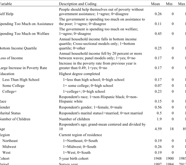
4.1 Descriptive statistics and description of all variables………..111
4.3 Logistic regression of pooled cross-sectional data predicting attitudes toward government involvement and government
spending on poverty……….121 4.4 Fixed-effects models of the effect of income loss on attitudes
toward government involvement in lessening poverty,
LIST OF FIGURES
Figure 1.1 – Poverty rate, 1959-2012.……….2 Figure 1.2 – Sibship size, Peabody picture vocabulary test score,
and first grade promotion....……….9 Figure 1.3 – Support for government spending on welfare and
assistance to the poor, 1984-2012………..12 Figure 2.1 – Weighted poverty rate and rate of welfare receipt
by dropout status, 1970-2010……….32 Figure 4.1 – Period and cohort variation in support for government involvement
and spending on lessening poverty………..115 Figure 4.2 – Overall period effects on support for government involvement
CHAPTER 1: INTRODUCTION AND OVERVIEW
In 1964, President Johnson famously declared an unconditional war on poverty, aiming not just to reduce the number of poor families or to make living in poverty more endurable, but to completely eliminate poverty. In the subsequent years, the federal government proposed a number of initiatives to help improve the education, health, and labor market outcomes of the poor. These initiatives gave birth to Medicare and Medicaid, and made a pilot food stamps program permanent. These initiatives also expanded Social Security benefits, increased benefits levels for Aid to Families with Dependent Children, and established the Jobs Corps and VISTA programs. These initiatives also created Head Start, Title I programs, and the now defunct Office of Economic Opportunity.
Social scientists at the time were optimistic that poverty could be greatly reduced or even eliminated. James Tobin, an adviser to President Johnson and an economics professor at Yale University, believed poverty could be completely eradicated in the US by 1976 (Tobin 1967). Robert Lampman, also an adviser to President Johnson and the founding director of the first federally funded poverty research center in the United States, was slightly less optimistic, arguing that poverty in the US could be completely eradicated, but not until 1980 (Lampman 1971).
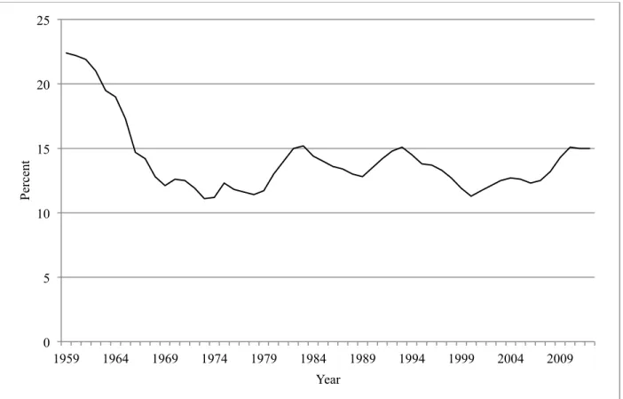
rate in the past 50 years. For the 40 years since 1973, the poverty rate has hovered around 13 percent, moving with economic booms and busts but never abating to the single digits.
Figure 1.1 Poverty Rate, 1959-2012.
Source: US Census Bureau, Current Population Survey, 1960-2013 Annual Social and Economic Supplements. 0
5 10 15 20 25
1959 1964 1969 1974 1979 1984 1989 1994 1999 2004 2009
P
erc
ent
At the same time, intergenerational mobility out of poverty has remained low. Children born in the poorest decile have a 31.5 percent chance of ending up in the poorest decile as an adult, and a 51.3 percent chance of ending up in the poorest quintile (Hertz 2005). For children from the poorest thirty percent of households, close to two-thirds will stay among the poorest thirty percent as adults. These numbers are astounding and disheartening: one in two children from the poorest tenth of households will end up among the poorest fifth as adults; only one in three children from the poorest thirty percent of households will move up beyond the poorest thirty percent of adults.
These trends are difficult to explain. In the mid-twentieth century, social scientists were optimistic that the poverty rate could be greatly diminished and the government took action to improve the chances of upward mobility for poor children. However, the poverty rate never dipped below one in ten and intergenerational mobility out of poverty remained limited. In turn, social scientists refocused their attention, seeking a better understanding of the social forces that maintain poverty. Unfortunately, progress has been slow and greatly hindered by methodological challenges.
poverty) is methodologically difficult. Given the complexity and the closely related nature of the issues affecting the poor, we are left with lingering questions.
This dissertation offers three pieces of empirical research that move forward our understanding of how social and economic contexts are related to poverty. In these papers, I investigate how social and economic contexts can lead to a biased understanding of what troubles the poor. I also examine how social and economic contexts can create divergent beliefs about the role of the government in lessening poverty. Taken as a whole, this dissertation offers a careful investigation of what ails the poor and what does not and also an improved understanding of the determinants of support for government action to lessen poverty.
Before providing a brief overview of each paper, it is worthwhile to consider why studying poverty is important. At the individual level, poverty has numerous consequences. Poverty leads to health problems, a shortened life expectancy, and an increased risk of criminal activity. These individual consequences have societal costs. Consider children raised in poor families. Children raised in poor families complete fewer years of education and have worse cognitive outcomes. As a result, the US economy wastes an immense amount of potential worker productivity and earnings. At the same time, children raised in poor families are more likely to be involved in crime and are also more likely to suffer from poor health. As a result,
expenditures on the criminal justice system and health care are artificially high, and worker productivity is again squandered because of losses to health limitations or imprisonment. Holzer et al (2007) estimate that childhood poverty costs the US about $500 billion per year through the loss of worker productivity and expenditures related to health and crime.
available consumers shrinks, demand for goods and services decreases, and economic growth slows. Consumers not directly affected by the increased poverty rate, weary of increasing economic hardship, become less likely to spend disposable income and worsen the decreased demand for goods and services. Conversely, decreases in the poverty rate leads to an increase in the number of people able to purchase goods and services, and can help stimulate economic growth (Bluestone & Harrison 2000).
Moreover, myths and misperceptions about poverty are common. In many instances, misperceptions are entirely misplaced. For example, a common misperception is that the
majority of poor are African American or that the majority of the poor are unemployed (Iceland 2012; O’Hare 1996). Both are inaccurate perceptions and are easily falsified. In other instances, misperceptions reign because of the absence of robust empirical research. The papers presented in this dissertation subject three common perceptions to rigorous analysis, assessing (1) to what extent the poor are poor because of low levels of educational attainment, (2) to what extent sibship size in low-income households shapes cognitive development and early educational achievement, and (3) to what extent economic hardship determines beliefs about lessening poverty.
Section 1.1: Overview of Dissertation
Paper 1: High School Dropouts, Poverty, and Welfare
Research on the determinants of poverty routinely highlights the role of education, arguing the poor are poor because of low levels of educational attainment. There is good reason to suspect that education is a determinant of poverty status. Educational attainment is an
employment status, and, importantly, poverty status. Notably, over one in four high school dropouts are in poverty compared to fewer than one in twenty college graduates.
Similarly, existing research proposes a number of mechanisms through which educational attainment has the potential to directly influence poverty status. Most obviously, human capital models show that increases in human capital are associated with increases in earnings. Those with less education acquire less human capital and are able to demand less from the labor market. As a result, they face an increased risk of poverty. Similarly, research on credentialism, social closures, and signaling shows how the presence of a degree can reap benefits for the credentialed even in the absence of skill differentials. In effect, individuals with less education may be formally limited to a smaller pool of available jobs or employers may doubt the abilities of the less educated, which in turn increases the risk of poverty.
However, the role of educational attainment in determining who is poor and who is not is muddied by nonrandom selection into different levels of educational attainment. Existing
research finds that various sociodemographic groups face an increased risk of not completing high school, or conversely, that various sociodemographic groups face an increased “risk” of completing college. In particular, family and neighborhood characteristics are an important determinant of high school completion. Ultimately, those who do not complete high school are likely different from high school graduates in meaningful and important ways in the same way that college graduates are likely different from high school graduates in meaningful and important ways.
measuring factors that contribute to selection into different levels of educational attainment. For example, parental behaviors influence the likelihood of completing high school. If a researcher’s analytic strategy does not account for parental behaviors, then findings will be inaccurate
because of omitted variable bias. Researchers could attempt to account for parental behaviors and other parental characteristics but they would need extremely detailed data to feel confident that the effect of educational attainment is not biased by unmeasured parental traits. This is only one example of the difficulty of measuring relevant characteristics, but there are many others. Consider the importance of neighborhoods. Neighborhoods have an important affect on educational attainment. Consequently, researchers need to be careful to account for neighborhood effects when considering the consequences of low levels of educational
attainment. However, neighborhood effects are notoriously difficult to observe and measure in survey data. Thus, researchers again run the risk of confounding neighborhood effects and educational attainment effects.
Similarly, we no longer need to worry about observing neighborhood characteristics because siblings live in the same neighborhood.
The research presented in this paper improves our understanding of the relationship between educational attainment and poverty. Increased educational attainment is routinely offered as a panacea for what ails the poor without a critical assessment of how social and economic contexts influence both poverty and educational attainment. This research offers a more nuanced and complete understanding of the extent to which dropping out of high school leads to poverty and welfare receipt.
Paper 2: Sibship Size, Cognitive Ability, and Early Educational Achievement
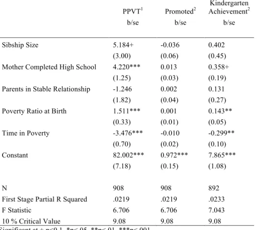
In the second paper in this dissertation, I consider whether variations in sibship size have meaningful consequences on cognitive ability or early educational achievement for children in low-income households. Figure 2 motivates this research. Panel A of Figure 2 shows variations in the average number of children in a household by mother’s income-to-poverty ratio. Panel B of Figure 2 shows variations in cognitive test scores by sibship size. Panel C of Figure 2 shows the percent of kindergarteners not promoted to first grade by sibship size. We see that poorer mothers have more children on average and that the number of siblings in a household is negatively associated with both cognitive ability and first grade promotion.
Research consistently finds that sibship size leads to worse education outcomes for children. Couple this finding with the fact that poor families on average have more children, and sibship size seems like an obvious candidate for a pathway from living in poverty to poor
Figure 1.2 Sibship Size, Peabody Picture Vocabulary Test Score, and First Grade Promotion.
Note: Data come from the Fragile Families and Child Wellbeing Study. Peabody Picture Vocabulary Test (PPVT) is a standardized test that measures verbal ability and scholastic aptitude.
Sibship size—like educational attainment—is not random. Thus, researchers must take selection effects seriously. The ability of Ordinary Least Squares regression models—the prevailing method used in past studies—to accurately capture the pathways from sibship size to outcomes is questionable. Therefore, I draw on a variety of multivariate approaches to examine the effects of sibship size on cognitive development and early educational achievement. Beyond OLS models, I conduct propensity score matching analysis and instrumental variable models. In the propensity score matching analyses, I pair children who are similar in meaningful ways and only differ in their number of siblings. In the instrumental variable models, I use an exogenous shock on sibship size—whether the mother of a poor household experiences a miscarriage—to obtain an unbiased sibship size effect.
Aside from selections effects and methodological concerns, there is an additional reason to suspect that sibship size may not matter or be less important in low-income households. Namely, the social and economic contexts that have the potential to lead to sibling penalties on cognitive development and early educational achievement may not be present in low-income households. For example, in middle class households an additional sibling may mean that parents elect to send their children to public school instead of private school. In low-income households, private school is unlikely an option regardless of sibship size. This research, therefore, adds to our understanding of how variations in social and economic contexts across income groups have the potential to yield different effects.
leads to adverse outcomes. It is critical to identify the actual mechanisms that lead to adverse outcomes. Yes, the poor on average have larger family sizes, and yes, poor children on average have worse education outcomes, but does sibship size negatively affect the education outcomes of poor children? This research offers an empirical test of a specific mechanism that may lead from living in poverty to worse outcomes.
Second, variations in cognitive ability and early educational achievement are associated with an array of deleterious consequences, including decreased educational attainment, increased delinquency, and future economic disadvantage. Accordingly, the effect of sibship size on cognitive ability and early educational achievement has important implications for our
understanding of achievement gaps between poor and non-poor children. If increases in sibship size negatively affect cognitive development and early educational achievement, then sibship size should help inform our understanding of achievement gaps in the same way that other family effects do.
Paper 3: Economic Hardship and Beliefs about Government Spending on Poverty
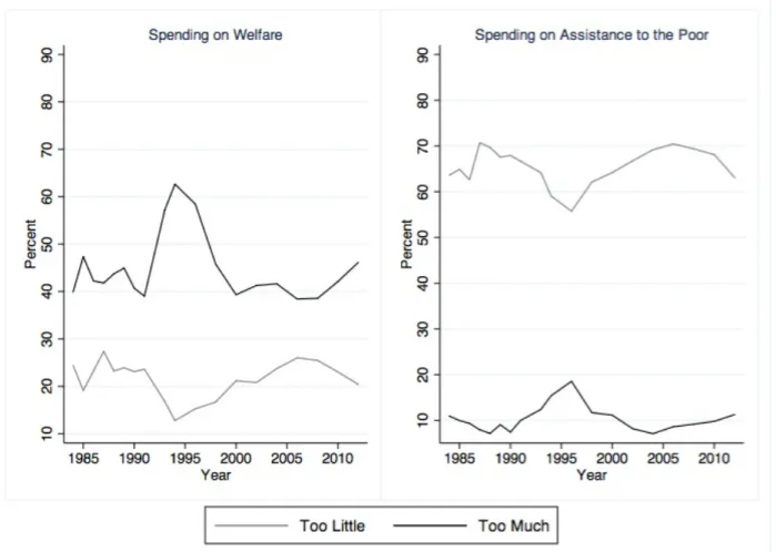
Opposition to antipoverty policies in the US is commonplace. However, opposition is inconsistent across policies. As an illustrative example, consider Figure 3, which shows support for government spending on welfare (left panel) and government spending on assistance for the poor (right panel) from 1984 to 2012. Here we see the percentage of people who believe the government spends too much on welfare, the percentage of people who believe the government spends too much on assistance for the poor, the percentage of people who believe the
government spends too little on welfare, and the percentage of people who believe the
believe the government spends too much on assistance for the poor. Yet, the plurality of people consistently believes the government spends too much on welfare.
There is an impressive body of research that attempts to explain the discrepancies
observed in Figure 3 and a similarly impressive body of research that investigates public support for government spending on poverty in general. Research on attitudes toward government spending on welfare and poverty largely rely on theories that emphasize the role of economic
Figure 1.3 Support for government spending on welfare and assistance to the poor, 1984-2012.
precarity. Unfortunately, past research has a large blind spot: it exclusively focuses on current conditions while overlooking past experiences. In effect, existing theories privilege current social and economic contexts—income, job security, educational attainment, macroeconomic climate— at the expense of past experiences. While current social and economic contexts are undoubtedly important—and existing research demonstrates the significant role of current social and
economic contexts—entirely overlooking the role of past contexts is imprudent.
In the third paper in this dissertation, I consider how views of the current are colored by the past. I draw on a rich body of literature from social psychology that shows experiences that occur during late adolescence and early adulthood can have a profound impact on life long attitudes and explore whether generational differences in beliefs exist net of current social and economic contexts. Are the cohorts who came of age during the war on poverty more or less likely to support government spending on poverty than the cohorts who came of age during welfare reform in the mid-1990s?
Existing research is further limited because it largely relies on cross-sectional data. As a result, sociological understandings of the fluidity of beliefs about government spending on poverty are incomplete. Are attitudes toward government spending on poverty fixed or do they respond to changes in economic contexts? When an individual experiences a change in her economic standing, do her beliefs follow? To answer these questions, I draw on longitudinal data to examine the stability and fluidity of beliefs about government spending on poverty. In
particular, I examine whether suffering an economic hardship produces an increase in support for government spending on poverty.
REFERENCES
Bluestone, Barry, and Bennett Harrison. 2000. Growing Prosperity: The Battle for Growth with Equity in the Twenty-First Century. Boston: Houghton Mifflin.
Hertz, Tom. 2005. Rags, Riches, and Race: The Intergenerational Economic Mobility of Black and White Families in the United States. In Unequal Chances: Family Background and Economic Success. Pp. 165-91. Eds. Samuel Bowles, Herbert Gintis, and Melissa Osborne Groves. New York: Russell Sage Foundation.
Holzer, Harry J., Diane Whitmore Schanzenbach, Greg J. Duncan, and Jens Ludwig. 2007. The Economic Costs of Poverty in the United States: Subsequent Effects of Children Growing Up Poor. Discussion Paper no. 1327-07. Institute for Research On Poverty, Madison WI. Iceland, John. 2012. Poverty in America: A Handbook. Berkeley: University of California Press. Lampman, Robert. 1971. Ends and Means of Reducing Income Poverty. Chicago: Markham. O’Hare, William P. 1996. A New Look at Poverty in America. Population Bulletin 51:1-48. Tobin, James. 1967. It Can Be Done! Conquering Poverty in the US by 1976. New Republic, 3
CHAPTER 2: THE SOCIOECONOMIC CONSEQUENCES OF DROPPING OUT: EVIDENCE FROM TWO COHORTS OF SIBLINGS
Introduction
The belief that dropping out of high school causes pervasive and persistent socioeconomic disadvantage is widespread. Viewed through the lens of cross-sectional
associations, the relationship between dropping out and future disadvantage is obvious—poverty rates, unemployment rates, and rates of welfare receipt for high school dropouts are significantly higher than the respective rates for high school graduates (Boisjoly et al 1998; Caspi et al 1998; Iceland 2012; National Center for Education Statistics 2012; US Census Bureau 2010). However, before concluding that dropping out is responsible for the increased risk of hardship, researchers must be careful to account for ways the population of dropouts differs from the population of high school graduates.
Put simply, high school dropouts likely face an elevated risk of socioeconomic disadvantage irrespective of their dropout status. The question, therefore, is not whether high school dropouts face an increased risk of disadvantage. They do. Instead, the question is whether dropping out of high school is responsible for the increased risk of disadvantage. If high school dropouts had completed high school, would they be any better off?
Research on the consequences of dropping out is surprisingly underdeveloped. Nearly three decades ago, Natriello, Pallas, and McDill (1986) called for researchers to investigate the social and economic effects of dropping out, writing:
dropping out . . . In order to do this, we need detailed information on the experiences and characteristics of dropouts before they left high school, as well as data on their labor market experiences … (p. 175).
This call for research on the consequences of dropping out has largely gone unanswered. Instead, discussions of the costs of dropping out have had to rely on cross-sectional associations (for example, see Rumberger 1987; Cheeseman Day & Newburger 2002). While cross-sectional associations reveal the level of disparity between high school graduates and high school
dropouts, they do not speak to the extent that dropping out contributes to the observed disparity. The absence of research is likely due to the difficulty of assessing the true costs of dropping out. Natriello, Pallas, and McDill point out the need for detailed data on dropouts before they leave school. Without such data, researchers run the risk of confounding dropout effects with the effects of early life social and economic contexts. This is particularly important because dropouts come disproportionately from already disadvantaged backgrounds (Alexander, Entwisle, & Horsey 1997; Brooks-Gunn, Guo, & Furstenberg 1993; Duncan et al 1998;
Rumberger 1987; Stearns and Glennie 2006), a strong determinant of both high school completion and economic hardship. The early and adolescent disadvantage that lead an individual to drop out likely also creates an increased risk of adult economic hardship. By the time an individual drops out of school, the risk of economic hardship may already be firmly in place.
estimation on within-family differences, the research presented here is better able to account for heterogeneity in the population of dropouts.
I make two additional contributions. First, I present conventional ordinary least squares (OLS) regression estimates of the effect of dropping out on future poverty and welfare receipt using the same data. By comparing conventional and within-family estimates, I am able to discern the extent to which differences in the backgrounds of dropouts are responsible for cross-sectional associations between dropping out and future socioeconomic disadvantage. In
particular, I am able to assess how unobserved characteristics may bias OLS estimates. Second, I analyze data from two cohorts of siblings, one cohort was high school age in the 1970s and the other was high school age in the 1990s. By comparing across cohorts, I am able to assess how the costs of dropping out have changed over time and also able to determine how the role of social background effects have increased or decreased in importance.
I first present arguments for why dropping out of high school likely leads to future poverty and welfare receipt, highlighting the role of skill differentials, credentialism, social closures, and signaling theory. I next discuss reasons for why the increased risk of disadvantaged faced by dropouts is likely overstated, emphasizing the difficulty of isolating an independent dropout effect using conventional OLS methods. I then outline the data, measures, and analytic strategy used in this paper. Lastly, I present findings from conventional OLS regression
Background
There are strong theoretical reasons to suspect that dropping out increases the risk of economic hardship net of background characteristics. First, it is possible that dropping out of high school produces an actual skill differential between dropouts and high school graduates. In effect, because dropouts do not complete all years of schooling, they do not develop the same level of skills and competencies. In this scenario, observed differences in poverty are indeed the result of dropping out. Had dropouts stayed in school, they would have acquired more skills and be able to demand more from the labor market.
The extent to which additional years of schooling leads to an increase in skills and an increase in future earnings is uncertain. The ambiguity is due to differences in who completes more years of education. Without experimental data, it is hard to assess whether differences in outcomes by educational attainment are the result of more years of education or the result of who completes more years of education. This is often referred to as “ability bias”—those with greater ability likely choose to complete more years of education. A large body of research has
attempted to identify the true effect of education on a variety of outcomes and has produced mixed evidence (for a review, see Card 1999). While most of this research examines the effects of educational attainment in general, the few studies that do consider high school dropouts in particular have produces similarly equivocal results.
the calendar year earn higher wages as a result of their increased schooling. However, these findings are strongly disputed and often used as an example of the shortcomings of instrumental variables. In particular, Bound, Jaeger, & Baker (1995) and Staiger and Stock (1997) show that the instrumental variable used by Angrist and Krueger—season of birth—explains little of the variation in educational attainment, making it too weak of an instrument to be informative.
Similarly, there is debate over whether more years of schooling produces greater skills and ability between dropouts and high school graduates. Alexander, Natriello, and Pallas (1985) compare cognitive development for dropouts and high school graduates. They find that
individuals who stay in school see more of an increase in cognitive skills than those who drop out. However, the effect sizes are modest—the average difference in cognitive test performance between dropouts and high school graduates was about one-tenth of a standard deviation. Additionally, even if staying in school does generate differences in skills and abilities, it is unclear whether that matters. Griffin, Kalleberg, and Alexander (1981) find that aptitude, class rank, and other school information has minimal and often insignificant effects on employment and other job related outcomes for high school graduates who enter the workforce directly upon high school completion. This conclusion is supported by a host of studies that find no effect or even a negative effect of high school grades on earnings (Kang & Bishop 1986; Miller 1998; Rosenbaum & Kariya 1991), and others who find that noncognitive traits—traits that are unlikely to be acquired through increased schooling—are much stronger predictors of labor market
Leaving aside these debates, we can also point to credentialism, social closures, and signaling theory as offering a theoretical motivation for an independent effect of dropping out on future disadvantage. We can think of credentialism as the extent to which employment or wages are allocated based on the possession of an education credential at the time of hiring, and social closures as the requirement of a degree to obtain a given position (Bills & Brown 2011; Bol & van der Werfhost 2011; Weeden 2002). Thus, a high school diploma could be important for a number of reasons: employers may see the credential as a status marker or regulations may require an employer to hire an individual with a high school diploma. If we imagine two potential job candidates that are equal in all ways except that Candidate A has a high school diploma and Candidate B does not, we could reasonably expect a perspective employer, because of credentialism or social closures, to prefer Candidate A to Candidate B. Ultimately, because of credentialism or social closure mechanisms, dropouts may be restricted to a smaller pool of available jobs or have limited potential wage growth. Thus, while a dropout may be qualified or have the needed abilities for a given employment opportunity, she will be passed over for the position because of the availability of someone with greater credentials or formal restrictions preventing her from obtaining the position.
A potential employer may also prefer Candidate A because the employer believes Candidate A’s high school diploma—or Candidate B’s lack of diploma—is representative of other characteristics and traits. According to signaling theory, employers value information about job candidates; however, because obtaining information about job candidates is costly,
available information—such as educational credentials—to infer the abilities and qualities of job applicants (Blaug 1976).
Signaling theory has important implications for the socioeconomic standing of dropouts. Specifically, while a given high school dropout may possess the same skills and knowledge as a high school graduate, employers may see the high school diploma—or the absence of a high school diploma—as signaling unobservable characteristics, leading employers to prefer high school graduates.
Heckman and Rubinstein (2001) offer a classic example of the possible role of signaling in influencing labor market outcomes. They show that persons with a GED earn less than persons who completed high school. They argue that while a GED shows that an individual has
comparable cognitive abilities to a high school graduate, it also signals to employers that GED holders “lack the ability to think ahead, to persists in tasks, or to adapt to their environments” (145). A similar conclusion holds for high school dropouts, only they also lack a certificate that asserts they possess cognitive abilities comparable to a high school graduate.
However, the evidence for signaling theory is far from decisive. Bills (1988) contends personality traits are as important to employers as formal education. Rosenbaum (2001) shows employers value soft skills over education related abilities. Cappelli (1995) contends employers rank character and attitude higher than education credentials. Moss and Tilly (2001) show employers privilege dependability and interpersonal communication above all else.
independently matters is less clear. Of particular concern is the ways in which dropouts and high school graduates differ beyond a high school diploma.
If individuals who drop out of high school are systematically different from those who complete high school, then researchers must be careful to account for these differences. If researchers are unable to account for differences between the two populations, there is reason to be concerned that observed differences between dropouts and high school graduates are due to unobserved variations. In effect, the observed differences in poverty and welfare receipt are not the result of dropping out, but instead are the result of the factors that lead individuals to drop out—the result of early life disadvantage and social contexts.
Past research has identified two populations that are at particular risk of dropping out: residents of economically disadvantaged neighborhoods and members of poor families.
According to research on neighborhood effects, all things being equal, children who grow up in neighborhoods with a high concentration of disadvantage are more likely to drop out of high school than children who grow up in more affluent neighborhoods. Results from experiments and quasi-experiments such as Gatreaux and Moving to Opportunity have generally confirmed this finding: individuals who move from high poverty neighborhoods to middle class neighborhoods are more likely to graduate from high school (DeLuca & Dayton 2009). Methodological debates notwithstanding, observational studies also confirm the basic tenets of neighborhood effects (Brooks-Gunn et al 1993; Crowder & South 2011; Harding 2003; Wodtke, Harding, & Elwert 2011).
If neighborhood effects could be easily measured in observational data, then the
effect net of neighborhood effects. Unfortunately, neighborhoods effects are diverse and not easily measured. For example, Brooks-Gunn and colleagues (1993) find that living in a
neighborhood with very few professional or managerial workers is associated with dropping out; Harding (2011) shows that neighborhood cultural context influences educational attainment; Crowder and South (2011) demonstrate that neighborhoods surrounding the immediate neighborhood of residence influence dropout rates. Overall, the diversity and complexity of neighborhood effects makes it difficult for researchers to confidently isolate a dropout effect using conventional OLS methods—should researchers include variables for the number of managers living in a neighborhood? how should a researcher operationalize neighborhood culture? what information about surrounding neighborhoods is relevant? Ruling out neighborhood effects with OLS methods and nonexperimental data is a near impossibility.
Similarly, the likelihood of dropping out varies by family socioeconomic status. Children and adolescents who grow up in poverty are less likely to complete high school (Alexander, Entwisle, & Horsey 1997; Duncan et al 1998). Numerous family characteristics influence
educational attainment, and, like the confounding effects created by neighborhood disadvantage, researchers must account for relevant family characteristics to confidently estimate an isolated dropout effect.
between “intact” and “nonintact” families (Astone & McLanahan 1991). To control for relevant family characteristics using conventional regression methods, researchers must account for an array of variables that are difficult to observe and measure, let alone operationalize.
In sum, for researchers to confidently isolate a dropout effect, they must account for the determinants of dropping out. Using conventional regression methods, this would take a heroic effort and implausibly rich data. If relevant determinants of dropping out are omitted or
measured inaccurately, then what appears to be a dropout effect on poverty may really be the result of omitted or poorly measured background characteristics. The implications are obvious and important: the same factors that lead adolescents to drop out may also lead to future poverty and welfare receipt—growing up in disadvantaged neighborhoods and families is strongly associated with adult poverty (Corcoran 1995; Duncan et al 1998; McLanahan 1985; Wagmiller et al 2006). For high school dropouts, the alternative to dropping out and poverty may be a high school diploma and poverty.
Data and Measures
Examining the consequences of dropping out requires detailed information on high school graduates and high school dropouts before they completed their education and also information on subsequent economic hardship. Because of the difficulty of measuring and observing all relevant background characteristics, a more robust method than conventional OLS methods is to compare siblings who have disparate education outcomes. I further elaborate on this point in the Analytic Strategy section of this paper, but for now it is sufficient to say that we need data that includes a sample of siblings and contains information on background
Longitudinal Study of Youth 1979 and 1997 (NLSY79 and NLSY97) cohorts meet these requirements.
The NLSY79 is a nationally representative sample of young adults who were between the ages of 14 and 22 when initially surveyed in 1979. From 1979 to 1994, follow-up waves were conducted annually. From 1994 to 2010, follow-up waves were conducted biennially. I transform the data to be structured by respondent age, not survey year. In effect, the baseline for all
respondent is when they are 18 years of age, not 1979; t2 is when respondents are 19 years old, not 1980; t3 is when respondents are 20 years old, and so on.
The NLSY79 is comprised of three subsamples: a cross-sectional sample of 6,111 youths, a supplemental sample of 5,295 Hispanic, black, and economically disadvantaged youths, and a military sample of 1,280 youths. The full sample in the baseline survey was 12,686. All eligible respondents within a household were included in the initial sample. The 11,406 civilian
respondents come from 7,490 unique households. 2,862 households include more than one NLSY79 respondent. The multi-respondent households include a total of 5,914 siblings.
The two outcomes, poverty status and welfare receipt, are both measured with indicator variables. Poverty status is measured using the official US Census Bureau thresholds with thresholds adjusted by family size. A respondent is defined as in poverty if his or her household income fell below the poverty threshold. A respondent is defined as having received welfare if he or she reported any cash income from Aid to Families with Dependent Children (up to 1996) or Temporary Assistance to Needy Families (after 1996), the main cash welfare programs in the US. Note that while poverty and welfare receipt are related, they are only weakly correlated to each other (0.27). This is because many people living in poverty elect to not participate (often out of ideological commitments or an inability to meet participation requirements), are unaware they are eligible, are ineligible despite having an income below the poverty line, or are unable to successfully enroll.
A respondent is defined as having dropped out if she has not completed high school and is not currently enrolled in school. To account for within-family heterogeneity, I include
measures of scholastic aptitude (standardized AFQT score), delinquency (regular use of alcohol or tobacco before the age of 18), and teen pregnancy (becoming a father or mother before the age of 18). The measures of within family heterogeneity help account for sibling differences that are associated with dropping out. For example, by including a measure of scholastic aptitude, we can be more confident that differences by dropout status are not really differences in scholastic aptitude. This issue is discussed in more detail in the analytic strategy. I also include
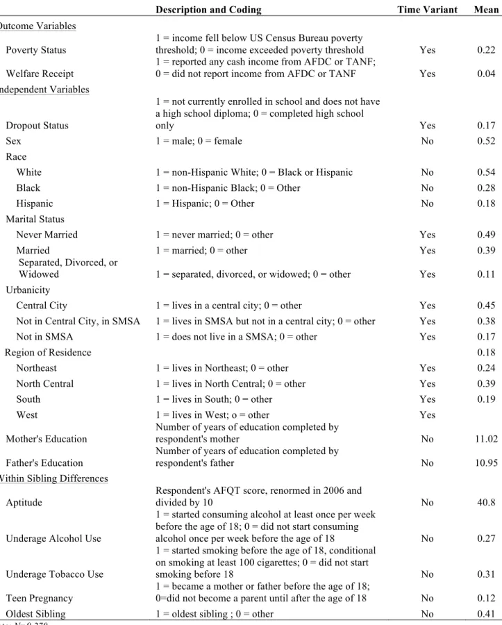
Table 2.1 Summary Statistics and Coding for All Variables.
!! Description and Coding Time Variant Mean
Outcome Variables Poverty Status
1 = income fell below US Census Bureau poverty
threshold; 0 = income exceeded poverty threshold Yes 0.22 Welfare Receipt
1 = reported any cash income from AFDC or TANF;
0 = did not report income from AFDC or TANF Yes 0.04 Independent Variables
Dropout Status
1 = not currently enrolled in school and does not have a high school diploma; 0 = completed high school
only Yes 0.17
Sex 1 = male; 0 = female No 0.52
Race
White 1 = non-Hispanic White; 0 = Black or Hispanic No 0.54
Black 1 = non-Hispanic Black; 0 = Other No 0.28
Hispanic 1 = Hispanic; 0 = Other No 0.18
Marital Status
Never Married 1 = never married; 0 = other Yes 0.49
Married 1 = married; 0 = other Yes 0.39
Separated, Divorced, or
Widowed 1 = separated, divorced, or widowed; 0 = other Yes 0.11 Urbanicity
Central City 1 = lives in a central city; 0 = other Yes 0.45 Not in Central City, in SMSA 1 = lives in SMSA but not in a central city; 0 = other Yes 0.38 Not in SMSA 1 = does not live in a SMSA; 0 = other Yes 0.17
Region of Residence 0.18
Northeast 1 = lives in Northeast; 0 = other Yes 0.24
North Central 1 = lives in North Central; 0 = other Yes 0.39
South 1 = lives in South; 0 = other Yes 0.19
West 1 = lives in West; o = other Yes
Mother's Education
Number of years of education completed by
respondent's mother No 11.02
Father's Education
Number of years of education completed by
respondent's father No 10.95
Within Sibling Differences Aptitude
Respondent's AFQT score, renormed in 2006 and
divided by 10 No 40.8
Underage Alcohol Use
1 = started consuming alcohol at least once per week before the age of 18; 0 = did not start consuming
alcohol once per week before the age of 18 No 0.27
Underage Tobacco Use
1 = started smoking before the age of 18, conditional on smoking at least 100 cigarettes; 0 = did not start
smoking before 18 No 0.31
Teen Pregnancy
1 = became a mother or father before the age of 18;
0=did not become a parent until after the age of 18 No 0.12
Oldest Sibling 1 = oldest sibling ; 0 = other No 0.41
(South, Northeast, Midwest, West). These additional covariates serve two purposes. First, they help ensure that observed differences between dropouts and high school graduates are not due to demographic differences in the two populations. Second, they help establish a baseline estimate for comparing between family estimates and within family estimates. Summary statistics and descriptions of the coding for each of these variables are presented in Table 2.1.
Analytic Strategy
To understand the relationship between dropping out and future poverty and welfare receipt, we must account for background effects that influence both the odds of dropping out and future risk of economic hardship. At issue is the nonrandom selection into dropping out. The decision to dropout is not independent of background characteristics. Models that omit background characteristics may produce biased estimates of future disadvantage.
Traditionally, researchers attempt to account for selection into dropping out through the use of controls in regression models. For example, poverty status for individual i in family f (Yif) is a function of dropout status (Xif), a vector of observed controlled variables (Zif), a family-specific error term (!f), and a random error term (!if), giving the equation:
[Equation 1] (Yif) = ! Xif + ! Zif + !f + !if
For example, assume a family has two children, Sibling A and Sibling B. Let Y1f be the poverty status for Sibling A, Y2f be the poverty status for Sibling B, X1f and X2f is dropout status for each sibling respectively, Z1f and Z2f are a vector of observed control variables, !1f and !2f are individual specific error terms, and !f is a family specific error term. The equation for Sibling A is
(Equation 2) Y1f = ! X1f + ! Z1f + !f + !1f The equation for Sibling B is
(Equation 3) Y2f = ! X2f + ! Z2f + !f + !2f If we subtract Equation 3 from Equation 2, we are left with
(Equation 4) Y1f – Y2f = ! (X1f – X2f) + ! (Z1f – Z2f) + !1f + !2f
Therefore, Equation 4 removes the family and neighborhood background characteristics shared by siblings, leaving sibling differences in poverty status as a function of dropping out of high school. In effect, because siblings experience the same neighborhoods, families, and other social backgrounds, we are able to account for these effects without observing, measuring, or
operationalizing them, which means the dropout effect is not biased by unobserved heterogeneity.
Researchers have used sibling fixed-effect models in a number of studies to address potential biases created by nonrandom allocation to different groups, such as the consequences of teenage pregnancy (experienced a teenage pregnancy versus did not experience a teenage
the family fixed-effects estimator. First, siblings are seldom the same age, and thus may
experience different social contexts. For example, family income or parenting styles may change over time. If these differences are correlated with dropping out, this could bias the dropout effect. Second, there may be differences among siblings that are correlated with dropping out. This has the potential to bias the dropout effect; however, to the extent that these differences are observed (such as including a proxy for scholastic aptitude as measured by standardized test scores), we can reduce this potential bias. Accordingly, I include measures of within family differences.
Additionally, because the outcomes of interest—poverty status and welfare receipt—are nonlinear and discrete variables, some fixed-effects strategies are not viable. Specifically, in a non-linear fixed-effects model, the number of nuisance parameters grows as sample size
increases, which produces biased covariate estimates. This is known as the incidental parameter problem. Consequently, I estimate both Chamberlain’s (1980) conditional logistic and linear probability models. The Chamberlain model estimates logistic fixed-effects using conditional likelihood functions, which excludes all siblings that do not vary on poverty or welfare status. The linear probability model, while adding ease of interpretation, produces predicted
probabilities that are not constrained between 0 and 1. As is common, I present the results from the linear probability models.
Figure 2.1 Weighted Poverty Rate and Rate of Welfare Receipt by Dropout Status, 1970-2010.
Note: Data from March Supplements of Current Population Survey, 1970-2010. For Panel A, n=3,785,905. For Panel B; n=3,488,487. Percentages are weighted to reflect cross-sectional national averages.
0 1 2 3 4 5 6 7 8
1970 1973 1976 1979 1982 1985 1988 1991 1994 1997 2000 2003 2006 2009
P
erc
ent
Year
(b) Welfare Receipt
Dropouts High School Graduates 0
5 10 15 20 25 30
1970 1973 1976 1979 1982 1985 1988 1991 1994 1997 2000 2003 2006 2009
P
erc
ent
Year
(a) Poverty
Findings
Figure 1 displays the percent poor and percent receiving welfare by dropout status from 1970-2010. In the top panel of Figure 1, Panel A, we see a sizable gap in poverty rates between dropouts and high school graduates. The trends in poverty rate largely mirror each other and the overall difference in poverty has changed little since the 1970s. In the bottom panel of Figure 1, Panel B, we see a large gap in the rate of welfare receipt between dropouts and high school graduates that narrows substantially over time. However, most of the narrowing occurs immediately following welfare reform in the mid-1990s and continues through 2010. Clearly, dropouts face an increased risk of poverty and welfare receipt, but would the risk of poverty or welfare receipt be eliminated if dropouts had completed high school?
Table 2.2 reports estimates of the effect of dropping out of high school on future poverty. Columns 1 through 4 present coefficients from conventional estimates (Equation 1). The first model estimates a baseline dropout effect and controls only for cohort. We see that dropping out increases the probability of living in poverty by 29 percent. Next, I add a set of standard
abl
e 2.2 T
and Hispanics face a higher risk of poverty than whites; increases in AFQT score are associated with a lower risk of poverty; delinquency is associated with an increased risk of poverty; teen parenthood increases the risk of poverty.
Column 5, Column 6, and Column 7 present coefficients from sibling fixed-effects estimates (Equation 4). In Column 5, I account for only demographic covariates. In Column 6, I account for demographic covariates and sibling differences in AFQT. In Column 7, I account for additional sibling differences that may influence dropping out—alcohol use during high school, tobacco use during high school, and becoming a parent during high school. When only
demographic variations are accounted for, dropping out increases the likelihood of living in poverty by 14 percent. Once sibling differences in aptitude, delinquency, and parenthood are modeled, the dropout effect is reduced to 11 percent (Column 7). Importantly, differences in scholastic aptitudes are associated with only a minimal change in the likelihood of poverty. The differences between the full random effects estimates presented in Column 4 and the full fixed-effects estimates presented in Column 7 demonstrate the difficulty of capturing background effects with proxy measures for social background and also reveal that traditional estimates overstate the effects of dropping out on poverty.
Table 2.3 reports estimates of the effect of dropping out on welfare receipt. I follow the same modeling strategy outlined above, first estimating four conventional models and then three sibling fixed-effects models. In the baseline model, Column 1, we see that dropping out of high school increases the likelihood of receiving welfare by 8 percent. Once basic demographic covariates are accounted for (Column 2), the dropout effect is largely unchanged. Controlling for scholastic aptitude (Column 3) results in a decrease in the likelihood of receipt of public
the dropout effect substantially. Compared to the model that omits background covariates
(Column 3), the full model reduces the likelihood of receiving public assistance by 45 percent.
By not completing high school, dropouts increase their probability of receiving welfare by 4
percent.
Columns 5, 6, and 7 of Table 2.3 report estimates of the probability of receiving welfare
from sibling fixed-effects models. Here we see consistency between the conventional and sibling
fixed-effects estimates. When we first account for only demographics in Column 4, we see that
dropping out increases the likelihood of welfare receipt by just over 4 percent. When we account
for differences in scholastic aptitude (Column 6), the likelihood of welfare receipt changes little.
Once we add measures of within-family heterogeneity (Column 7), the dropout effect is reduced
to less than 3 percent. The random and fixed-effects estimates from Columns 4 and 7 differ
modestly. Unobserved background effects play only a minor role in the probability of welfare
receipt for high school dropouts.
The above results indicate that dropping out of high school has a significant and
important effect on future poverty and welfare receipt. However, it is possible that the dropout
effect and the role of background characteristics have changed over time. Accordingly, I run the
analyses separately by cohort to examine possible differential effects.
Table 2.4 shows estimates of the effect of dropping out on future poverty for the older
cohort only, and Table 2.5 shows estimates of the effect of dropping out on future welfare receipt
for the older cohort only. For both tables, I follow the same modeling strategy as reported in
Table 2.2 and Table 2.3. In the baseline model (Column 1), we see that dropping out increases
the probability of poverty by close to 30 percent. Once demographic covariates are added to the
abl
e 2.4 T
he E ff ec t of D roppi ng O ut on P ove rt
y, 1979 Cohort
abl
e 2.5 T
he E ff ec t of D roppi ng O ut on W el fa re Re ce ipt
, 1979 Cohort
ability reduce the risk of poverty substantially (31 percent), and the full set of observed
background covariates further reduces the risk of poverty. In the full model, the risk of poverty for dropouts is 16 percent. In Column 5, Column 6, and Column 7, I report estimates from the sibling fixed-effects models. When we only account for demographic covariates, the risk of poverty is 14 percent for high school dropouts. When we add sibling differences in scholastic ability to the model, the risk of poverty is reduced to 12 percent. When we add sibling
differences in alcohol use, tobacco use, and teen parenthood to the model, the risk of poverty is reduced to 11 percent. Importantly, we observe notable differences between the random effects estimate and the sibling fixed-effects estimate, indicating that unobserved background
characteristics are biasing the dropout effect.
We observe a similar pattern for the effect of dropping out on welfare receipt for the older cohort (Table 2.5). In the baseline model, dropping out increases the risk of welfare by 9 percent for the older cohort. Accounting for demographic covariates does little, but the full set of background covariates reduces the risk to fewer than 5 percent. The sibling fixed-effects models report modestly lower estimates of the effect of dropping out. In the full sibling fixed-effects model, dropping out increases the risk of welfare receipt by 3 percent. The minimal differences between estimates presented in Columns 4 and 7 of Table 2.5 again indicate that the dropout effect on welfare is only biased minimally by unobserved background characteristics.
estimates were more similar for the older cohort, the sibling fixed-effects estimate is
substantially different for the younger cohort. Once unobserved background characteristics and sibling differences are modeled, the risk of poverty is a little over 6 percent, nearly half of the conventional estimate.
The findings reported in Table 2.6 and Table 2.7 have three important implications. First, for the younger cohort, estimates of the dropout effect are biased by unobserved heterogeneity. While dropping out still increases the risk of poverty for the younger cohort, much of the risk comes from unobserved differences between dropouts and high school graduates. Second,
background characteristics that lead to dropping out are becoming more important in determining poverty across cohorts. Third, the effect of dropping out on poverty is decreasing over time.
We also see important differences between cohorts in the risk of welfare receipt for dropouts. In the conventional models, the risk of welfare receipt for dropouts in the younger cohort goes from over 4 percent in the baseline model to under 2 percent in the full model. The dropout effect in the full model, however, approaches statistical significance but is not
abl
e 2.6 T
he E ff ec t of D roppi ng O ut on P ove rt
y, 1997 Cohort
abl
e 2.7 T
he E ff ec t of D roppi ng O ut on W el fa re Re ce ipt
, 1997 Cohort
abl
e 2.8 T
he E ff ec t of D roppi ng O ut on P ove rt y f or A ge s 18
-30, 1979 Cohort
Lastly, to further compare the risk of poverty for high school dropouts across cohorts, I include a final set of models (Table 2.8). In these models, I examine the risk of poverty for the older cohort, limiting the sample to the years where respondents are below the age of 30—the oldest age where data are available for the younger cohort. This set of models allows me to compare the risk of poverty for the older and younger cohorts during the same age range. Overall, we observe a pattern similar to the previously reported findings. The dropout effect is larger for the older cohort even when limited to the same age range. A t-test confirms that the observed differences in the risk of poverty are statistically different across cohorts in a one tailed test at .05 or at .10 in a two tailed test (t =1.71) Moreover, even when the sample is restricted for younger ages for the older cohort, the unobserved background covariates explain less of the difference between the conventional estimates and sibling fixed-effects estimates. This further suggests that unobserved covariates are more influential for the younger cohort.
Discussion
There is widespread public concern about the economic fate of dropouts. These concerns are well intentioned, but lack empirical support because of the difficulties of estimating an unbiased dropout effect. Dropouts differ from high school graduates in more ways than just a high school diploma, and researchers must be careful to account for these differences or they run the risk of misattributing background effects to dropout effects.
In this study, I present both conventional regression estimates and sibling fixed-effects estimates on the effect of dropping out on poverty and welfare receipt, a surprisingly
fixed-effects estimates attenuate this finding: when model estimation is based on within-family differences, I find smaller estimates of the consequences of dropping out on future poverty and welfare receipt. However, the dropout effect remains substantial and significant. The
implications of this are clear and important: by not completing high school, dropouts are increasing the probability of experiencing poverty and receiving welfare.
The research presented here also unearths an important temporal change in the consequences of dropping out. For the older cohort, those who were high school age in the 1970s, the conventional estimates and sibling fixed-effects estimates are more closely aligned. For the younger cohort, those who were high school age in the 1990s, we observe large
differences between the conventional and within-family estimates.
For the younger cohort, conventional estimates substantially overstate the cost of dropping out. Unobserved background characteristics are important and are able to explain nearly half of the increased probability of poverty among dropouts and completely explain away the increased probability of welfare. While cohort difference in welfare receipt among dropouts is likely due to welfare reform, a takeaway remains: for the younger cohort, once unobserved background characteristics are accounted for, dropouts are no more likely to receive welfare than high school graduates.
However, it remains to be seen if this disparity across cohorts persists. The NLSY97 cohort is only in early adulthood in the most recent survey years. It is possible that over time the conventional and sibling fixed-effects estimates will converge and more closely resemble the estimates of the older cohort.
If the estimates do not converge over time, then we will need to reconsider our
attempt to measure the effects of educational attainment. For the older cohort, the bias in the
conventional estimates is minimal. This is consistent with other work that attempts to measure
the amount of bias in OLS estimates of educational effects on earnings (Card 1999). For the
younger cohort, if the gap between the within family estimates and between family estimates
remains large, social scientists will have more difficulty estimating the effects of educational
attainment.
These findings have important policy implications. If unobserved background
characteristics explained the differences in the increased likelihood of poverty or welfare receipt
among dropouts, then policies aimed solely at increasing graduation rates would be misguided.
Instead, policies would need to address the background determinants that make dropouts differ
from high school graduates. This would create a difficult task for policymakers—policies aimed
at family changes are more challenging than policies aimed at school changes. However, this is
not the case. A dropout effect remains even after accounting for unobserved differences. Thus,
policies that are able to increase graduation rates should reduce the rate of poverty among
students who would have dropped out otherwise.
Recent education reforms largely push for an increase in standards and added
requirements for high school graduation. The findings presented here support past calls for a
careful reconsideration of how to balance improving the quality of education without increasing
the dropout rate (Alexander et al 1985; McDill et al 1986). Consider high school exit
examinations. Approximately two-thirds of all American high school students must pass an exit
examination to earn their diploma (Warren 2007). High school exit examinations are no doubt
well intentioned and there are many good reasons to ensure that high school graduates meet
dropout rates among low-ability students (Jacob 2001). Students who would have completed
high school if not for the exit examination now face an increased risk of poverty.
Finally, the results indicate that a large portion of the disparity between high school
graduates and high school dropouts is explained by social and economic background. This
speaks to the limit of schools and also supports recent shifts in anti-poverty policies that focus on
intervention at the community level (e.g. Promise Neighborhoods and Promise Zones). Efforts to
improve the socioeconomic position of high school dropouts do not need to be limited to
classroom walls.
This study also suggests potentially fruitful avenues for future research. First, this
research shows cohort differences in the consequences of dropping out, but is unable to speak to
the source of these differences. Over the past forty years, the labor market has changed
dramatically, seeing a large growth in job precarity (Kalleberg 2011). Thus, it seems likely that
changes in the labor market drive cohort differences; however, additional research is needed.
Additionally, this research demonstrates that dropping out has an effect on poverty independent
of background characteristics, but does not address the root cause of this difference. What is it
about dropping out? Is it the loss of a credential? Diminished human capital and skills? Research
that explicitly tests the mechanisms that lead from dropping out to poverty is needed. Lastly,
while the effect of dropping out on poverty and welfare receipt is understudied, the effect of
dropping out on other social outcomes is common. In particular, a large body of research
examines the effects of dropping out on crime. The analytic strategy and findings presented in
this study offer a potentially productive line of investigation for criminologists interested in the
REFERENCES
Aaronson, Daniel. 1998. Using Sibling Data to Estimate the Impact of Neighborhoods on Children’s Educational Outcomes. Journal of Human Resources 33:915-46.
Alexander, Karl L., Doris R. Entwisle, and Carrie S. Horsey. 1997. From First Grade Forward: Early Foundations of High School Dropout. Sociology of Education 70:80-107.
Alexander, Karl L., Gary Natriello, and Aaron M. Pallas. 1985. For Whom the School Bell Tolls: The Impact of Dropping Out on Cognitive Performance. American Sociological Review 50:409-20.
Angrist, Joshua D., and Alan B. Krueger. 1991. Does Compulsory School Attendance Affect Schooling and Earnings? Quarterly Journal of Economics 106:979-1014.
Astone, Nan Marie, and Sara S. McLanahan. 1991. Family Structure, Parental Practices and High School Completion. American Sociological Review 56:309-20.
Bills, David B. 1988. Educational Credentials and Hiring Decisions: What Employers Look for in New Employees. Research in Social Stratification and Mobility 7:71-97.
Bills, David B., and David K. Brown. 2011. New Directions in Educational Credentialism. Research in Social Stratification and Mobility 29:1-4.
Blaug, Mark. 1976. The Empirical Status of Human Capital Theory: A Slightly Jaundiced Survey. Journal of Economic Literature 14:827-55.
Boisjoly, Johanne, Kathleen Mullan Harris, and Greg J. Duncan.1998. Trends, Events, and Duration of Initial Welfare Spells. Social Service Review 72:466-92.
Bol, Thijs, and Herman G. van der Werfhost. 2011. Signals and Closures by Degrees: The Education Effect across 15 European Countries. Research in Social Stratification and Mobility 29:119-32.
Bound, John, David A. Jaeger, and Regina M. Baker. 1995. Problems with Instrumental
Variables Estimation When the Correlation Between the Instruments and the Endogenous Explanatory Variable is Weak. Journal of the American Statistical Association 90:443-50.
Bowles, Samuel, and Herbert Gintis. 2002. Schooling in Capitalist America Revisited. Sociology of Education 75:1-18.
Bronars, Stephen, and Jeffrey Grogger. 1994. The Economic Consequences of Unwed
Motherhood: Using Twin Births as a Natural Experiment. American Economic Review 84:1141-56.