The Rosetta all-atom energy function for macromolecular modeling and design
Rebecca F. Alford,1 Andrew Leaver-Fay,2 Jeliazko R. Jeliazkov,3 Matthew J. O’Meara,4 Frank P. DiMaio,5 Hahnbeom Park,6 Maxim V. Shapovalov,7 P. Douglas Renfrew,8,9 Vikram K. Mulligan,6 Kalli Kappel,10 Jason W. Labonte,1 Michael S. Pacella,11 Richard Bonneau,8,9 Philip Bradley,12 Roland L.
Dunbrack Jr.,7 Rhiju Das,13 David Baker,6 Brian Kuhlman,2 Tanja Kortemme,14 Jeffrey J. Gray1,2§
1 Department of Chemical and Biomolecular Engineering, Johns Hopkins University, 3400 North
Charles Street, Baltimore, Maryland 21218, United States
2 Department of Biochemistry and Biophysics, University of North Carolina at Chapel Hill, 120 Mason
Farm Road, Chapel Hill, North Carolina 27599, United States
3 Program in Molecular Biophysics, Johns Hopkins University, 3400 North Charles Street, Baltimore,
Maryland 21218, United States
4 Department of Pharmaceutical Chemistry, University of California at San Francisco, 1700 Fourth
Street, San Francisco, California 94158, United States
5 Department of Biochemistry, University of Washington, J-Wing Health Sciences Building, Box
357350, Seattle, Washington 98195, United States
6 Department of Biochemistry, University of Washington, Molecular Engineering and Sciences, 4000
15th Ave NE, Seattle, Washington 98195, United States
7 Institute for Cancer Research, Fox Chase Cancer Center, 333 Cottman Avenue, Philadelphia,
Pennsylvania 19111, United States
8 Department of Biology, Center for Genomics and Systems Biology, New York University, 100
Washington Square East, New York, New York 10003
9 Center for Computational Biology, Flatiron Institute, Simons Foundation, 162 5th Avenue, New York,
New York 10010, United States
10 Biophysics Program, Stanford University, 450 Serra Mall, Stanford, California 94305, United States 11 Department of Biomedical Engineering, Johns Hopkins University, 3400 North Charles Street,
Baltimore, Maryland 21218, United States
12 Computational Biology Program, Fred Hutchinson Cancer Research Center, 1100 Fairview Avenue
North, Seattle, Washington 98109, United States
13 Department of Biochemistry, Stanford University, B400 Beckman Center, 279 Campus Drive,
Stanford, California 94305, United States
14 Department of Bioengineering and Therapeutic Sciences, University of California at San Francisco,
San Francisco, California 94158, United States
Abstract
Over the past decade, the Rosetta biomolecular modeling suite has informed diverse biological questions and engineering challenges ranging from interpretation of low-resolution structural data to design of nanomaterials, protein therapeutics, and vaccines. Central to Rosetta’s success is the energy function: a model parameterized from small molecule and X-ray crystal structure data used to approximate the energy associated with each biomolecule conformation. This paper describes the mathematical models and physical concepts that underlie the latest Rosetta energy function, beta_nov15. Applying these concepts, we explain how to use Rosetta energies to identify and analyze the features of biomolecular models. Finally, we discuss the latest advances in the energy function that extend capabilities from soluble proteins to also include membrane proteins, peptides containing non-canonical amino acids, carbohydrates, nucleic acids, and other macromolecules.
Table of Contents Graphic
Keywords
Introduction
Proteins adopt diverse three-dimensional conformations to carry out the complex mechanisms of life. Their structures are constrained by the underlying amino acid sequence1 and stabilized by a fine balance between enthalphic and entropic contributions to non-covalent interactions.2 Energy functions that seek to approximate the energy of these interactions are fundamental to computational modeling of biomolecular structures. The goal of this paper is to describe the energy calculations used by the Rosetta macromolecular modeling program:3 we explain the underlying physical concepts, mathematical models, latest advances, and application to biomolecular simulations.
Energy functions are based on Anfinsen’s hypothesis that native-like protein conformations represent unique, low-energy, thermodynamically stable conformations.4 These folded states reside in minima on the energy landscape, and they have a net favorable change in Gibbs free energy, which is the sum of contributions from both enthalpy (∆H) and entropy (∆S) relative to the unfolded state. To follow these heuristics, macromolecular modeling programs require a mathematical function that can discriminate between the unfolded, folded, and native-like conformations. Typically, these functions are a linear combination of terms that compute energies as a function of various degrees of freedom.
The earliest macromolecular energy functions combined a Lennard-Jones potential for van der Waals interactions5–7 with harmonic torsional potentials8 that were parameterized using force constants from vibrational spectra of small molecules.9–11 These formulations were first applied to investigating the structures of hemolysin,12 trypsin inhibitor,13 and hemoglobin14 and have now diversified into a large family of commonly used energy functions such as AMBER,15 DREIDING,16 OPLS,17 and CHARMM.18,19 Many of these energy functions also rely on new terms and parameterizations. For example, faster computers have enabled the derivation of parameters from ab initio quantum calculations.20 The maturation of X-ray crystallography and NMR protein structure determination
methods has enabled development of statistical potentials derived from per-residue, inter-residue, secondary-structure, and whole structure features.21–28 Additionally, there are alternate models of electrostatics and solvation, such as a Generalized Born approximation of the Poisson-Boltzmann equation29 and polarizable electrostatic terms that accommodate varying charge distributions.30
The first version of the Rosetta energy function was developed for proteins by Simons et al.31 Initially, it used statistical potentials describing individual residue environments and frequent residue-pair interactions derived from the Protein Databank (PDB).32 Later, the authors added terms for packing of van der Waals spheres, hydrogen bonding, secondary-structure, and van der Waals interactions to improve the performance of ab initio structure prediction.33 These terms were for low-resolution modeling, meaning
that the scores were dependent on only the coordinates of the backbone atoms and that interactions between the side chains were treated implicitly.
to reach several milestones in structure prediction and design including accurate ab initio structure prediction.40 hot-spot prediction,41,42 protein—protein docking,43 and specificity redesign44 as well as the first de novo designed protein backbone not found in nature45 and the first computationallydesigned new protein—protein interface.46
The Rosetta energy function has changed dramatically since it was last described in complete detail by Rohl et al.47 in 2004. It has undergone significant advances ranging from improved models of hydrogen bonding48 and solvation,49 to updated evaluation of backbone50 and rotamer conformations.51 Along the way, these developments have enabled Rosetta to address new biomolecular modeling problems including refinement of low-resolution X-ray structures,52 development of protein binders,53 and the design of vaccines,54 biomineralization peptides,55 self-assembling materials,56 and enzymes that perform new functions.57,58 Instead of arbitrary units, the energy function is now also calibrated to compute energies in kcal/mol. The details of these energy function advances are distributed across code comments, methods development papers, application papers, and individual experts, making it challenging for Rosetta developers and users in both academia and industry to learn the underlying concepts. Moreover, members of the Rosetta community are actively working to generalize the all-atom energy function for use in different contexts59,60 and for all biomolecules including RNA,61 DNA,62,63 small-molecule ligands,64 non-canonical amino acids and backbones,65–67 and carbohydrates,68 further encouraging us to reexamine the underpinnings of the energy function. Thus, there is a need for an up-to-date description of the current energy function.
In this paper, we describe the concepts and calculations underlying the current Rosetta all-atom energy function called beta_nov15. Our discussion aims to expose the physical and mathematical details of the energy function required for rigorous understanding. In addition, we explain how to apply the computed energies to analyze structural models produced by Rosetta simulations. We hope this paper will provide critically needed documentation of the energy methods as well as an educational resource to help students and scientists interpret the results of these simulations.
Computing the total Rosetta energy
The Rosetta energy function approximates the energy of a biomolecule conformation. This quantity, called
∆𝐸total, is computed from a linear combination of energy terms 𝐸' which are calculated as a function of geometric degrees of freedom, 𝛩, chemical identities, aa, and scaled by a weight on each term, 𝑤, as shown in Eq. 1.
∆𝐸total = '𝑤'𝐸'(𝛩', aa') (1)
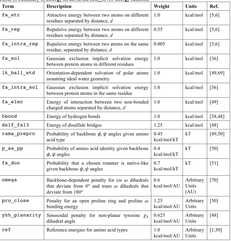
Table 1: Summary of Energy terms in the beta_nov15 energy function
Term Description Weight Units Ref.
fa_atr Attractive energy between two atoms on different residues separated by distance, d
1.0 kcal/mol [5,6]
fa_rep Repulsive energy between two atoms on different residues separated by distance, d
0.55 kcal/mol [5,6]
fa_intra_rep Repulsive energy between two atoms on the same residue, separated by distance, d
0.005 kcal/mol [5,6]
fa_sol Gaussian exclusion implicit solvation energy between protein atoms in different residues
1.0 kcal/mol [36]
lk_ball_wtd Orientation-dependent solvation of polar atoms assuming ideal water geometry
1.0 kcal/mol [49,69]
fa_intra_sol Gaussian exclusion implicit solvation energy between protein atoms in the same residue
1.0 kcal/mol [36]
fa_elec Energy of interaction between two non-bonded
charged atoms separated by distance, d 1.0 kcal/mol [49]
hbond Energy of hydrogen bonds 1.0 kcal/mol [38,48]
dslf_fa13 Energy of disulfide bridges 1.25 kcal/mol [48]
rama_prepro Probability of backbone 𝜙, 𝜓 angles given amino acid type
0.45
kcal/mol/kT
kT [49,50]
p_aa_pp Probability of amino acid identity given backbone
𝜙, 𝜓 angles 0.4 kcal/mol/kT
kT [50]
fa_dun Probability that a chosen rotamer is native-like given backbone 𝜙, 𝜓 angles
0.7
kcal/mol/kT
kT [51]
omega Backbone-dependent penalty for cis 𝜔 dihedrals that deviate from 0° and trans 𝜔 dihedrals that deviate from 180°
0.6 kcal/mol/AU Arbitrary Units (AU) [70]
pro_close Penalty for an open proline ring and proline 𝜔 bonding energy
1.25
kcal/mol/AU Arbitrary Units [50]
yhh_planarity Sinusoidal penalty for non-planar tyrosine 𝜒3 dihedral angle 0.625 kcal/mol/AU Arbitrary Units [48]
ref Reference energies for amino acid types 1.0
kcal/mol/AU
Arbitrary Units
Terms for atom-pair interactions
van der Waals interactions are short-range attractive and repulsive forces that vary with atom-pair distance. Whereas attractive forces result from the cross-correlated motions of electrons in neighboring non-bonded atoms, repulsive forces occur because electrons cannot occupy the same orbitals by the Pauli exclusion principle. To model van der Waals interactions, Rosetta uses the Lennard-Jones (LJ) 6-12 potential5,6 which calculates the interaction energy of atoms 𝑖 and 𝑗 in different residues given their summed atomic radii 𝜎',7,a atom-pair distance, 𝑑',7, and the geometric mean of well depths, 𝜖',7 (Eq. 2). The atomic radii and well depths are derived from small molecule liquid phase data optimized in context of the energy model.49
𝐸vdw(𝑖, 𝑗) = 𝜀',7 >?,@
A?,@
BC
− 2 >?,@
A?,@
F
(2)
Rosetta splits the LJ potential at the function’s minimum (𝑑',7 = 𝜎',7) into two components that can be weighted separately: attractive (fa_atr) and repulsive (fa_rep). By decomposing the function this way, we can alter component weights without changing the minimum-energy distance or introducing any derivative discontinuities. Many conformational sampling protocols in Rosetta take advantage of this splitting by slowly increasing the weight of the repulsive component to traverse rugged energy landscapes and to prevent structures from unfolding during sampling.71
The repulsive van der Waals energy, fa_rep, varies as a function of atom-pair distance. At short distances, atomic overlap results in strong forces that lead to large changes in the energy. The steep 1/𝑑',7BC
term can cause poor performance in minimization routines and overall structure prediction and design calculations.72,73 To alleviate this problem, we weaken the repulsive component by replacing the 1/𝑑',7BC term with a softer linear term when 𝑑 ≤ 0.6𝜎',7. The term is computed using the atom-type specific parameters 𝑚',7 and 𝑏',7 which are fit to ensure derivative continuity at 𝑑 = 0.6𝜎',7 After the linear component, the function transitions smoothly to the 6-12 form until 𝑑',7 = 𝜎, where it reaches zero and remains zero (Eq. 3; Fig. 1A).
𝐸rep(𝑖, 𝑗) = 𝑤',7conn
𝑚',7 𝑑',7 + 𝑏',7 𝑑',7 ≤ 0.6𝜎',7
𝜀',7 >?,@
A?,@
BC
− 2 >?,@
A?,@
F
+ 1 0.6𝜎',7 < 𝑑',7 ≤ 𝜎',7
0 𝜎',7 < 𝑑',7
',7 (3)
Rosetta also includes an intra-residue version of the repulsive component, fa_intra_rep, with the same functional form as the fa_rep term (Eq. 3). We include this term because the knowledge-based rotamer energy (fa_dun, below) under-estimates intra-residue collisions.
polynomial function, 𝑓poly 𝑑',7 after 4.5 Å to transition the standard Lennard-Jones functional form smoothly to zero. These smooth derivatives are necessary to ensure that bumps do not accumulate in the distributions of structural features at inflections points in the energy landscape during conformational sampling with gradient-based minimization (Sheffler 2006, Unpublished).
𝐸atr= 𝑤',7conn
– 𝜀',7 𝑑',7 ≤ 𝜎'7
𝜀',7 >A?,@
?,@
BC
− 2 >?,@
A?,@
F
𝜎',7 < 𝑑',7 ≤ 4.5 Å
𝑓`abc 𝑑',7 4.5 Å ≤ 𝑑',7 ≤ 6.0 Å
0 6.0 Å ≤ 𝑑',7
',7 (4)
All three terms are multiplied by a connectivity weight 𝑤',7conn to exclude the large repulsive energetic contributions that would otherwise be calculated for atoms separated by fewer than four chemical bonds (Eq. 5). This weight is common to molecular force fields that assume covalent bonds are not formed or broken during a simulation. Rosetta uses four chemical bonds as the “crossover” separation when 𝑤',7conn transitions from zero to one (rather than the three chemical bonds used by traditional force fields) to limit the effects of double-counting due to knowledge-based torsional potentials.
𝑤',7conn=
0 𝑛',7bonds ≤ 3
0.2 𝑛',7bonds = 4
1 𝑛',7bonds ≥ 5
(5)
The comparison between Eq. 2 and the modified LJ potential (Eq. 3-4) is shown in Fig. 1A and Fig. 1B.
Figure 1: Van der Waals and electrostatics energies
Comparison between pairwise energies of non-bonded atoms computed by Rosetta and the form computed by traditional molecular mechanics force fields. Here, the interaction between the backbone nitrogen and carbon are used as an example. (A) Lennard-Jones van der Waals energy with well-depths 𝜖Nbb= 0.162 and 𝜖Cbb= 0.063 and atomic radii 𝑟Nbb=
1.763 and 𝑟Cbb= 2.011 (red) and Rosetta fa_rep(blue). (B) Lennard-Jones van der Waals energy (red) and Rosetta
Electrostatics. Non-bonded electrostatic interactions arise from forces between fully and partially charged atoms. To evaluate these interactions, Rosetta uses Coulomb’s Law with partial charges originally taken from CHARMM and adjusted via a group optimization scheme (Table S3).49 Coulomb’s law is a pairwise term commonly expressed in terms of the distance between atoms 𝑖 and 𝑗 (𝑑',7), dielectric constant 𝜖, partial atomic charges for each atom 𝑞' and 𝑞7, and Coulomb’s constant, 𝐶o = 322 Å kcal/mol e-2 (with e being the elementary charge) (Eq. 6).
𝐸Coulomb(𝑖, 𝑗) =qrs?s@
t B
A?,@u (6)
To approximate electrostatic interactions in biomolecules, we modify the potential to account for the difference in dielectric constant between the protein core and solvent-exposed surface.74 Specifically, we substitute the constant 𝜖 in Eq. 6 with a sigmoidal function 𝜖 𝑑',7 that increases from 𝜖core= 6 to
𝜖solvent = 80 when the atom-pair distance is between 0 Å and 4 Å (Eq. 7-8):
𝜖 𝑑',7 = 𝑔 A?,@
x 𝜖core+ 1 − 𝑔 A?,@
x 𝜖solvent (7)
𝑔 𝑥 = 1 + 𝑥 +zCu exp(−𝑥) (8)
As with the van der Waals term, we make several heuristic approximations to adapt this calculation for simulations of biomolecules. To avoid strong repulsive forces at short distances, we replace the steep gradient with the constant 𝐸elec(𝑑min) when 𝑑',7 < 1.45 Å. Next, since the distance-dependent dielectric assumption results in dampened long-range electrostatics, for speed we truncate the potential at 𝑑max = 5.5 Å and we shift the Coulomb curve by subtracting a 1 𝑑maxC term to shift the potential to zero at 𝑑
max (Eq. 9).
𝐸elec(𝑖, 𝑗, 𝑑',7) =qrs?s@
t(A?,@)
B A?,@u −
B
Amaxu 𝑑 ≤ 𝑑max
0 𝑑max < 𝑑
(9)
We use cubic polynomials, 𝑓polyelec,low(𝑑',7) and 𝑓polyelec,high(𝑑',7) to smooth between the traditional form and our adjustments while avoiding derivative discontinuities. The energy is also multiplied by the connectivity weight, 𝑤',7conn (Eq. 5). The final modified electrostatic potential is given by Eq. 10 and compared to the standard form in Fig. 1C.
𝐸fa_elec = 𝑤',7conn
𝐸elec(𝑖, 𝑗, 𝑑min) 𝑑',7 < 1.45 Å
𝑓polyelec,low(𝑑',7) 1.45 Å ≤ 𝑑',7 < 1.85 Å 𝐸elec(𝑖, 𝑗, 𝑑',7) 1.85 Å ≤ 𝑑',7 < 4.5 Å
𝑓polyelec,hi(𝑑',7) 4.5 Å ≤ 𝑑',7 < 5.5 Å
0 5.5 Å ≤ 𝑑',7
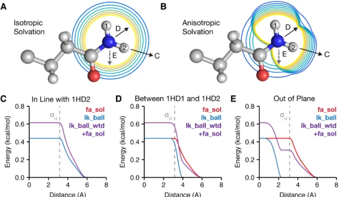
Solvation. Native-like protein conformations minimize the exposure of hydrophobic side chains to the surrounding polar solvent. Unfortunately, explicitly modeling all the interactions between solvent and protein atoms is computationally expensive. Instead, Rosetta represents the solvent as bulk water based upon the Lazaridis-Karplus (LK) implicit Gaussian exclusion model.36 Rosetta's solvation model has two
components: an isotropic solvation energy, called fa_sol, that assumes bulk water is uniformly distributed around the atoms (Fig. 2A) and an anisotropic solvation energy, called lk_ball_wtd, that accounts for specific waters nearby polar atoms that form the solvation shell (Fig. 2B).
Figure 2: A two component Lazaridis-Karplus solvation model
Rosetta uses two energy terms to evaluate the desolvation of protein side chains: an isotropic (fa_sol) and anisotropic (lk_ball_wtd) term. (A) and (B) demonstrate the difference between isotropic and anisotropic solvation of the NH2 group by CH3 on the asparagine side chain. The contours vary from low energy (blue) to high energy (yellow). The arrows represent the approach vectors for the pair potentials shown in C-E. In the bottom panel, we compare fa_sol, lk_balland lk_ball_wtdenergies for the solvation of the NH2 group on asparagine for three different approach angles: (C) in line with the 1HD2 atom, (D) along the bisector of the angle between 1HD1 and 1HD2 and (E) vertically down from above the plane of the hydrogens (out of plane).
The isotropic (Lazaridis-Karpus) model36 is based on the function 𝑓desolv that describes the energy required to desolvate (remove contacting water) an atom 𝑖 when approached by a neighboring atom 𝑗. In Rosetta, we exclude Lazaridis-Karplus’ ∆𝐺ref term because we implement our own reference energy (discussed later). The energy of the atom-pair interaction varies with separation distance 𝑑',7, experimentally determined vapor-to-water transfer free energies ∆𝐺free, summed atomic radii 𝜎
',7, correlation length 𝜆, and atomic volume of the desolvating atom 𝑉7 (Eq. 11).
𝑓desolv = −𝑉7 ∆ƒ?free
C„…u†?>?u
exp − A‡>?,@
†?
C
At short distances, fa_rep prevents atoms from overlapping; however, many protocols briefly down-weight or disable the fa_rep term. To avoid scenarios where 𝑓desolv encourages atom-pair overlap in the absence of fa_rep, we smoothly increase the value of the function to a constant at close distances when the van der Waals spheres overlap (𝑑',7 = 𝜎',7). At large distances, the function asymptotically approaches zero; therefore, we truncate the function at 6.0 Å for speed. We also transition between the constants at short and long distances using distance-dependent cubic polynomials 𝑓`abcsolv,lowand 𝑓polysolv,high with constants
𝑐o = 0.3 Å and 𝑐B = 0.2 Å that define a window for smoothing. The overall desolvation function is given by Eq. 12.
𝑔desolv =
𝑓desolv(𝑖, 𝑗, 𝜎',7) 𝑑',7 ≤ 𝜎',7 − 𝑐o 𝑓`abcsolv,low(𝑖, 𝑗, 𝑑',7) 𝜎',7 − 𝑐o < 𝑑',7 ≤ 𝜎',7+ 𝑐B
𝑓desolv 𝑖, 𝑗, 𝑑',7 𝜎',7+ 𝑐B < 𝑑',7 ≤ 4.5 Å 𝑓polysolv,high(𝑖, 𝑗, 𝑑',7) 4.5 Å < 𝑑',7 ≤ 6.0 Å
0 6.0 Å < 𝑑',7
(12)
The total isotropic solvation energy (Eq. 13), fa_sol, is computed as a sum including atom j desolvating atom i and vice-versa and scaled by the previously-defined connectivity weight.
𝐸fa_sol = 𝑤',7conn 𝑔
desolv 𝑖, 𝑗 + 𝑔desolv(𝑗, 𝑖)
',7 (13)
Rosetta also includes an intra-residue version of the isotropic solvation energy, fa_intra_sol, with the same functional form as the fa_sol term (Eq. 13).
A recent innovation (2016) is the addition of an energy term (lk_ball_wtd) to model the orientation-dependent solvation of polar atoms. This anisotropic model increases the desolvation penalty for occluding polar atoms near sites where waters may form hydrogen bonding interactions. For polar atoms, we subtract off part of the isotropic energy of Eq. 13 and then add the anisotropic energy to account for the position of the desolvating atom relative to hypothesized water positions.
To compute the anisotropic energy, we first calculate the set of ideal water sites around atom i, 𝒲' =
𝝂'B, 𝝂'C, … . This set contains 1 to 3 water sites, depending on the atom type of atom i. Each site is 2.65 Å from atom 𝑖 and has an optimal hydrogen-bond geometry, and we consider the potential overlap of a desolvating atom j with each water. The overlap is considered negligible until the van der Waals sphere of the desolvating atom j (radius 𝜎7) touches the van der Waals sphere of the water at site k (radius 𝜎Œ), and then the term smoothly increases over a zone of partial overlap of approximately 0.5 Å. Thus, for each water site, 𝑘, with coordinates 𝒗',•, we compute an occlusion measure 𝑑•C to capture the gap between the hypothetical water and the desolvating atom 𝑗 (Eq. 14), using the offset Ω = 3.7 Å2 to provide the ramp-up buffer.
𝑑•C = 𝒓
7 − 𝒗',• C
− 𝜎Œ+ 𝜎7 C+ Ω (14)
Next, we find the soft minimum of 𝑑•C over all water sites in 𝒲
𝑑minC (𝑖, 𝑗) = − ln exp −𝑑 •C
•∈𝒲? (15)
Then, 𝑑minC and Ω are used to compute a damping function 𝑓
lkfrac (Eq. 16) that varies from zero when the
desolvating atom is at least a van der Waals distance from any preferred water site to one when the desolvating atom overlaps a water site by more than ~ 0.5 Å.
𝑓lkfrac 𝑖, 𝑗 =
1 𝑑minC 𝑖, 𝑗 < 0
1 − Aminu ',7 “
C
0 ≤ 𝑑minC 𝑖, 𝑗 < Ω
0 Ω ≤ 𝑑minC 𝑖, 𝑗
(16)
We calculate the anisotropic energy of desolvating a polar atom 𝐸lk_ball by scaling the desolvation function
𝑔desolv by the damping function 𝑓lkfrac and an atom-type specific weight 𝑤aniso that is typically ~0.7 (Eq. 17). The amount of isotropic solvation energy subtracted is 𝑔desolv multiplied by 𝑤iso, where 𝑤iso is an atom-type specific weight typically ~0.3 (Eq. 18; the total weight on the isotropic contribution through both fa_sol and lk_ball_wtd terms is thus ~0.7). The isotropic and anisotropic components are then summed to yield a new desolvation function, ℎdesolv (Eq. 19).
𝐸lk_ball(𝑖, 𝑗) = 𝑤aniso,'𝑔desolv(𝑖, 𝑗)𝑓lkfrac(𝑖, 𝑗) (17)
𝐸lk_ball_iso(𝑖, 𝑗) = −𝑤iso,' 𝑔desolv(𝑖, 𝑗) (18)
ℎdesolv(𝑖, 𝑗) = 𝐸lk_ball_iso(𝑖, 𝑗) + 𝐸lk_ball(𝑖, 𝑗) (19)
Like fa_sol, the energy of desolvating atom 𝑖 by atom 𝑗 and then 𝑗 by 𝑖 are summed to yield the overall lk_ball_wtd energy (Eq. 20) but only counting the desolvation of polar, hydrogen-bonding heavy atoms (O,N) defined as the set 𝒫. Fig. 2 shows a comparison between fa_sol, the lk_ball term (Eq. 17), and the sum of fa_sol and lk_ball_wtd for the example of an asparagine NH2 desolvated from three different approach angles. As the approach angle varies, the sum of lk_ball_wtd and fa_sol creates a larger desolvation penalty when waters sites are occluded and a smaller penalty otherwise, relative to the fa_sol term alone.
𝐸lk_ball_wtd = 𝑤',7connℎ
desolv 𝑖, 𝑗 + 7∈𝒫𝑤',7connℎdesolv 𝑗, 𝑖
'∈𝒫 (20)
Hydrogen bonding. Hydrogen bonds are partially covalent interactions that form when a nucleophilic heavy atom donates electron density to a polar hydrogen.75 At short ranges (< 2.5 Å), they exhibit
geometries that maximize orbital overlap.76 The interactions between hydrogen bonding groups are also partially described by electrostatics. While this hybrid covalent-electrostatic character is complex, it is crucial for capturing the structural specificity that underlies protein folding, function, and interactions. Rosetta calculates the energy of hydrogen bonds using fa_elec and a term called hbond that evaluates energies based on the orientation preferences of hydrogen bonds found in high-resolution crystal structures.38,48 To derive this model, we curated intra-protein polar contacts from ~8,000 high resolution
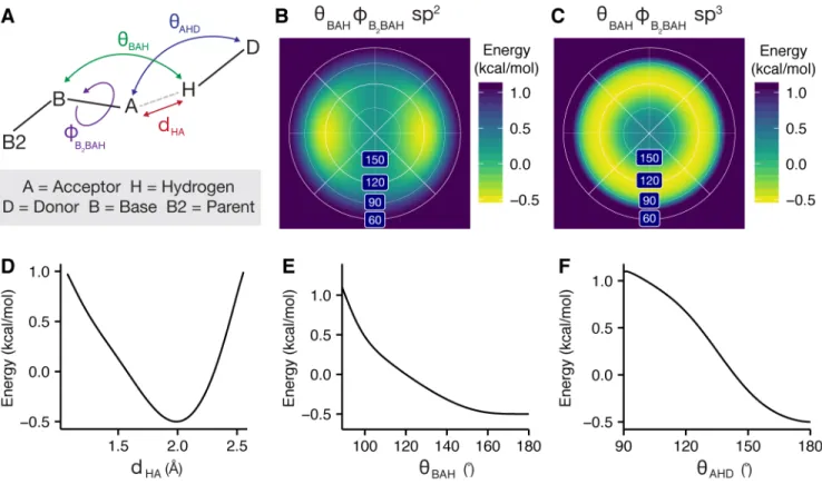
distributions from Top8000. The resulting hydrogen bonding energy is evaluated for all pairs of donor hydrogens, H, and acceptors, A, as a function of four degrees of freedom (Fig. 3A): (1) the distance between the donor and acceptor, 𝑑—˜ (2) the angle formed by the donor, acceptor, and donor-heavy atom,
𝜃˜—š (3) the angle formed by the acceptor’s parent atom (“base”) B, acceptor, and the donor, 𝜃›˜— and (4) the torsion, 𝜙›u›˜—, formed by the donor, acceptor, and two subsequent parent atoms B and B2. (Fig.
3A). B, the parent atom of A,is the first atom on the shortest path to the root atom (e.g. Cα). The B2 atom
of A is the parent atom of B (e.g., the sp2 plane is defined by B2, B, and A)
Figure 3: Orientation-dependent hydrogen bonding model
(A) Degrees of freedom evaluated by the hydrogen bonding term: acceptor—donor distance, 𝑑—˜, angle between the base, acceptor and hydrogen 𝜃›˜—, angle between the acceptor, hydrogen, and donor, 𝜃˜—š, and dihedral angle corresponding to rotation around the base—acceptor bond, 𝜙›u›˜—. (B) Lambert-azimuthal projection of the 𝐸hbond›u›˜— energy landscape for an sp2 hybridized acceptor.48 (C) 𝐸hbond›u›˜— energy landscape for an sp3 hybridized acceptor. Example
energies for the histidine imidazole ring acceptor hydrogen bonding with a protein backbone amide: (D) energy vs. the acceptor—donor distance, 𝐸hbond—˜ (E) energy vs. the acceptor-hydrogen-donor angle, 𝐸hbond˜—š (F) energy vs. the base-acceptor—hydrogen angle, 𝐸hbond›˜— .
To avoid over-counting, side-chain to backbone hydrogen bonds are excluded if the backbone group is already involved in a hydrogen bond. For speed, the component terms have simple analytic functional forms (Fig. 3B-F; Supporting Information Eq. S1-7). The term is also multiplied by two atom-type specific weights, 𝑤— and 𝑤˜, that account for the varying strength of hydrogen bonds. The overall model is given by Eq. 21 where the 𝐸hbond›u›˜— term depends on the orbital hybridization of the acceptor, 𝜌. Finally,
𝐸hbond= 𝑤—𝑤˜𝑓 𝐸hbond—˜ 𝑑
—˜ + 𝐸hbond˜—š 𝜃˜—š + 𝐸hbond›˜— (𝜃›˜—) + 𝐸hbond›u›˜— 𝜌, 𝜙›u›˜— , 𝜃›˜—
—,˜
(21)
𝑓 𝑥 =
𝑥 𝑥 < −0.1
−0.025 +zC+ 2.5𝑥C −0.1 ≤ 𝑥 < 0.1
0 0.1 ≤ 𝑥
(22)
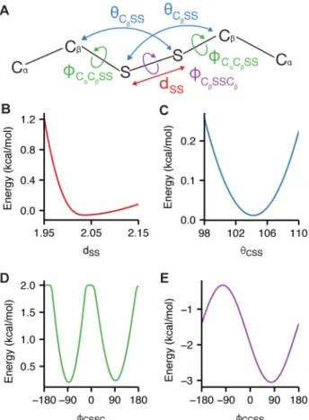
Disulfide bonding. Disulfide bonds are covalent interactions that link sulfur atoms in cysteine residues. Typically, in Rosetta, we rely on a tree-based kinematic system78,79 to keep bond lengths and angles fixed so that we may sample conformation space changing only torsions. For this reason, we do not generally need terms that evaluate bond-length and bond-angle energetics. However, with disulfide bonds and proline (below), the extra bonds cannot be represented with a tree (since a tree graph is acyclic), and thus must be treated explicitly. Thus, disulfide bonds are a special case of inter-residue covalent contact that requires a representation with more degrees of freedom. To evaluate disulfide bonding interactions, Rosetta identifies pairs of cysteines that have covalent bonds linking the Sγ atoms. Then, Rosetta computes the energy of these interactions using an orientation-dependent model called dslf_fa13.48 The model was derived by curating intra-protein disulfide bonds from Top8000 and identifying features using kernel density estimates. For speed, the feature distributions are modeled using skewed Gaussian functions and a mixture of 1, 2, and 3, von Mises functions (Supporting Information Eq. S8-11).
The overall disulfide energy is computed as a function of six degrees of freedom (Fig. 4) that map to four component energies. First, the geometry of the sulfur-sulfur distance 𝑑•• is evaluated by 𝐸dslf•• 𝑑 . Second, the angle formed by either 𝐶žB or 𝐶žC with S-S bond is evaluated by 𝐸dslfq•• 𝜃 . Third, the dihedral formed by either 𝐶ŸB𝐶žB or 𝐶ŸC𝐶žC with the S-S bond is evaluated by 𝐸dslfq q¡•• 𝜙
. Finally, the dihedral formed by 𝐶žB, 𝐶žC and the S-S bond is evaluated by 𝐸dslfq¡••q¡(𝜙). The complete disulfide bonding energy
evaluated for all S-S pairs is given by Eq. 23.
𝐸dslf_fa13= 𝐸dslf•• 𝑑
•• + 𝐸dslfq•• 𝜃q¡¢•• + 𝐸dslf
q•• 𝜃
q¡u•• + 𝐸dslf
q q¡•• 𝜙
q ¢q¡¢•• +
•¢,•u
𝐸dslfq q¡•• 𝜙
q uq¡u•• + 𝐸dslf
q¡••q¡( 𝜙
Figure 4: Orientation-dependent disulfide bonding model
(A) Degrees of freedom evaluated by the disulfide bonding energy: sulfur—sulfur distance, 𝑑££, angle between the 𝛽 -carbon and two sulfur atoms, 𝜃q••, dihedral corresponding to rotation about the 𝛼-Carbon and sulfur bond 𝜙q q¡••, and
dihedral corresponding to rotation about the S—S bond 𝜙••. (B) 𝐸dslf•• (C) 𝐸dslfq•• (D) 𝐸dslf
q q¡•• (E) 𝐸
dslf q¡••q¡.
Terms for Protein Backbone and Side Chain Torsions
Rosetta evaluates backbone and side-chain conformations in torsion space to greatly reduce the search domain and increase computational efficiency. Traditional molecular mechanics force fields describe torsional energies in terms of sines and cosines which have at times performed poorly at reproducing the observed backbone-dihedral distributions in unstructured regions.80 Instead, Rosetta uses several
knowledge-based terms for torsion angles that are fast approximations of quantum effects and more accurately model the preferred conformations of protein backbones and side-chains.
Ramachandran. To evaluate backbone 𝜙 and 𝜓 angles, we defined an energy term called rama_prepro based on Ramachandran maps for each amino acid, using torsions from 3,985 protein chains with a resolution ≤ 1.8 Å, R-factor ≤ 0.22 and sequence identity ≤ 50%.81 Amino acids with low electron density (in the bottom 25th percentile of each residue type) were removed from the data set. The resulting ~581,000
residues were used in adaptive kernel density estimates51 of Ramachandran maps with a grid step of 10˚ for both 𝜙 and 𝜓. Residues preceding proline are also treated separately because they exhibit distinct 𝜙, 𝜓
Information includes a detailed discussion of why interpolation is performed on the backbone torsional energies rather than the probabilities (Fig. S3, Eqs. S12-13).
𝐸rama_pre_pro =
− ln 𝑃reg(𝜙', 𝜓'|aa') C-terminus or 𝑖+1 is not a proline − ln 𝑃prepro(𝜙', 𝜓'|aa') 𝑖+1 is a proline
' (24)
Figure 5: Backbone torsion energies
The backbone-dependent torsion energies are demonstrated for the lysine residue. (A) The 𝜙 angle is defined by the backbone atoms 𝐶'‡B− 𝑁 − 𝐶Ÿ− 𝐶 and the 𝜓 angle is defined by 𝑁 − 𝐶Ÿ− 𝐶 − 𝑁'ªB. (B) rama_prepro energy of lysine without a proline at 𝑖+1. (C) rama_prepro energy of lysine with a proline at i+1. (D) p_aa_pp energy of
lysine.
Backbone design term. Rosetta also computes the likelihood of placing a specific amino acid side chain given an existing 𝜙, 𝜓 backbone conformation. This term, called p_aa_pprepresents the propensity of observing an amino acid relative to the other 19 canonical amino acids.84 The knowledge-based propensity, 𝑃 aa 𝜙, 𝜓 (Eq. 25) was derived using the adaptive kernel density estimates for 𝑃(𝜙, 𝜓|aa)
and Bayes’ rule. The equation for p_aa_pp is given in Eq. 26 (Fig. 5D).
𝑃 aa 𝜙, 𝜓 = « 𝜙, 𝜓 aa « aa
« 𝜙, 𝜓 aa¬ «(aa¬)
aa- (25)
𝐸p_aa_pp= − ln «aa« aa®𝜙®, 𝜓®
¯
® (26)
Side-chain conformations. Protein side chains mostly occupy discrete conformations (rotamers) separated by large energy barriers. To evaluate rotamer conformations, Rosetta derives probabilities from the 2010 backbone-dependent rotamer library (dunbrack.fccc.edu/bbdep2010), which contains the frequencies, means, and standard deviations of individual 𝜒 angles for each 𝜒 angle 𝑘 of each rotamer of each amino acid type.51 The probability has three components: (1) observing a specific rotamer given the
backbone dihedral angles (2) observing specific 𝜒 angles given the rotamer and (3) observing the terminal χ angle distribution, which is either Gaussian-like or continuous when the terminal 𝜒 angle is sp2
hybridized (Eq. 27). Here, 𝑇 represents the number of rotameric 𝜒 angles + 1.
The 2010 rotamer library distinguishes between rotameric and non-rotameric torsions. A torsion is rotameric when the third of the four atoms defining the torsion is sp3 hybridized (i.e. preferring ~60°, ~180° and ~-60°, with steep energy barriers between the wells), If the last 𝜒 torsion is rotameric, probability 𝑝 𝜒² 𝜙, 𝜓,rot,aa is fixed at one. On the other hand, a torsion is non-rotameric its third atom is sp2 hybridized: the library describes its probability distribution continuously, instead. The category of semi-rotameric amino acids with both rotameric and non-rotameric dihedrals encompasses eight amino acids: Asp, Asn, Gln, Glu, His, Phe, Tyr, and Trp.85
The probability of each rotamer 𝑃 rot 𝜙, 𝜓, aa is derived from the same dataset as the Ramachandran maps described above. The probabilities were identified using adaptive kernel density estimation and the same dataset is used to estimate the mean and standard deviation for each 𝜒 dihedral in the rotamer, and
𝜇µ¶ and 𝜎µ¶, as functions of the backbone dihedrals, allowing us to compute a probability for the 𝜒 values using Eq. 28.
𝑃(𝜒•|𝜙•, 𝜓•,rot)= exp −BC
µ¶‡·¸¶ ¹,º rot,aa)
>¸¶ ¹,º rot,aa) C
(28)
This formulation is reminiscent of the Gaussian distribution, except that it is missing the normalization coefficient of 2𝜋𝜎µ¶ 𝜙, 𝜓 rot,aa) ‡B C. After taking the log of this probability, the term resembles Hooke’s law where the spring constant is given by 𝜎µ‡C¶ 𝜙, 𝜓 rot,aa).
The full form of fa_dun is given by Eq. 29 as a sum over all residues r. The difference between the rotameric- and semi-rotameric models is also shown in Fig. 6.
𝐸fa_dun= − ln 𝑃 rot® 𝜙®, 𝜓®, aa® + BC µ¶,¯>‡·¸¶ ¹¯,º¯¼a½¯,¾¾¯)
¸¶ ¹¯,º¯rot¯,¾¾¯)
C
•±²¯ +
®
− ln 𝑃 𝜒²¯,® 𝜙®, 𝜓®, rot®, aa® (29)
The energy from − ln 𝑃 rot® 𝜙®, 𝜓®, aa® is computed using bicubic-spline interpolation;
𝑃 𝜒²¯,® 𝜙®, 𝜓®, rot®, aa® is computed using tricubic-spline interpolation. To save memory,
Figure 6: Energies for side-chain rotamer conformations
The Dunbrack rotamer energy, fa_dun, is dependent on both the 𝜙 and 𝜓 backbone torsions and the 𝜒 side-chain torsions. Here, we demonstrate the variation of fa_dun when the backbone is fixed in an α-helical conformation with 𝜙 = -57˚ and 𝜓 = -47˚, and the 𝜒 values can vary. 𝜒B is shown in blue, 𝜒C shown in red and 𝜒3 shown in green. (A) 𝜒 -dependent Dunbrack energy of methionine with an sp3-hybridized terminus (B) 𝜒-dependent energy of glutamine with an sp2-hybridized 𝜒3 terminus. 𝜒B, 𝜒C and 𝜒3 of methionine and 𝜒B and 𝜒C of glutamine express rotameric behavior while
𝜒3 of the latter expresses broad non-rotameric behavior.
Terms for special case torsions
Peptide bond dihedral angles, 𝜔, remain mostly fixed in a cis- or trans- conformation and depend on the backbone f and y angles. Since the electron pair on the backbone nitrogen donates electron density to the electrophilic carbonyl carbon, the peptide bond has partial double bond character. To model this barrier to rotation, Rosetta implements a backbone-dependent harmonic penalty centered near 0° for cis and 180°
for trans (Fig. 7A). This energy, called omega, is evaluated on all peptide bonds in the biomolecule (Eq. 30). The means and standard derivations of w, 𝜇¿and 𝜎¿, respectively, are backbone (f,y) dependent, as given by kernel regressions of w on f and y.70
𝐸omega = ln F C„B − ln > B
À ¹¯,º¯aa¯) C„ +
¿¯‡·À ¹¯,º¯aa¯)u
C>Àu ¹¯,º¯aa¯)
Figure 7: Special case torsion energies
Rosetta implements three additional energy terms to model torsional degrees of freedom with acute preferences. (A) Omega torsion corresponding to rotation about C-N (B) Proline secondary omega torsion corresponding to rotation about C-N related to the C-𝛿 in the ring. (C) Tyrosine terminal 𝜒 torsion. (D) Omega energy (E) Proline closure energy (F) Tyrosine planarity energy.
Most Rosetta protocols only search over simple torsions within chains and rigid-body degrees of freedom between chains. However, proline’s side chain requires special treatment because its ring cannot be represented by a kinematic tree.86 Therefore, Rosetta implements a proline closure term, called pro_close (Fig. 7B). There are two components to this energy, shown in Eq. 31. First, there is a torsional potential that operates on the dihedral formed by Or-1–Cr-1–Nr–Cδ,r, called 𝜔®¬ given the observed mean 𝜇¿- and standard deviation 𝜎¿¬, where i is the residue index. This term keeps the Cδ atom in the
peptide plane. Second, to ensure correct geometry for the two hydrogens bound to Cδ, we build a virtual atom, Nv, off Cδwhose coordinate is controlled by 𝜒3 (Fig. 7B). The pro_close term seeks to align the virtual Nv atom, directly on top of the real backbone nitrogen. The N–Cδ–Cγ bond angle and the N–Cδ
bond length are restrained to their ideal values.
𝐸pro_close =
¿¯-‡· À-u
>À-u +
𝐍¯‡𝐍Ã,¯ u
>N,NÃu 𝑟 is not N-terminus
𝐍¯‡𝐍Ã,¯ u
>N,NÃu 𝑟 is N-terminus
®∈Pro (31)
Tyrosine also requires special treatment for its 𝝌𝟑 angle because the hydroxyl hydrogen prefers to be in the plane of the aromatic ring.87 To enforce this preference, Rosetta implements a sinusoidal penalty to model the barrier to a 𝜒3 angle that deviates from planarity. This tyrosine hydroxyl penalty is called yhh_planarity (Eq. 32; Fig. 7C).
Terms for modeling non-ideal bond lengths and angles
Cartesian bonding energy. Recently, modeling Cartesian degrees of freedom during gradient-based minimization has been shown to improve Rosetta’s ability to refine low-resolution structures determined by X-ray crystallography and cryo-electron microscopy,52 as well as its ability to discriminate near-native conformations in the absence of experimental data.88 These data suggest that capturing non-ideal bond lengths and angles can be important for accurate modeling of minimum-energy protein conformations. To accommodate, Rosetta now allows these “non-ideal” angles and lengths to be included as additional degrees of freedom in refinement and includes a Cartesian-minimization mode where atom coordinates are explicit degrees of freedom in optimization.
To evaluate the energetics of non-ideal bond lengths, angles and planar groups, an energy term called cart_bonded represents the deviation of these degrees of freedom from ideal using harmonic potentials (Eq. 32-34). Here, 𝑑' is a bonded-atom-pair distance with 𝑑',o as its ideal distance, 𝜃' is a bond angle with
𝜃',o as its ideal angle, and 𝜙' is a bond torsion or improper torsion with 𝜙',o as its ideal value and 𝜌' as its periodicity. The ideal bond lengths and angles89,90 were selected based on their ability to rebuild side chains observed in crystal structures (Kevin Karplus & James J. Havranek, unpublished); they were subsequently modified empirically.50 The spring constants for the angle and length terms are from CHARMM32.19 Finally, all planar groups and the Cβ “pseudo-torsion” are constrained using empirically derived values and spring constants:
𝐸cart_length =BC Ç'ÈB𝑘',length(𝑑' − 𝑑',o)C (33)
𝐸cart_angle =B
C 𝑘',angle(𝜃' − 𝜃',o) C É
'ÈB (34)
𝐸cart_torsion = BC 𝑘',torsion 𝑓wrap 𝜙' − 𝜙',o,C„Ê
?
C Ë
'ÈB (35)
The function 𝑓wrap(𝑥, 𝑦) wraps 𝑥 to the range [0, 𝑦). To avoid double counting in the case of 𝐸cart_torsion, the spring constant 𝑘',torsion is zero when the torsion 𝜙' is being scored by either the rama or fa_dun terms.
Terms for Protein Design
Design reference energy. The terms above are sufficient for comparing different protein conformations with a fixed sequence. However, protein design simulations compare the relative stability of different amino acid sequences given a desired structure to identify models that exhibit a large free energy gap between the folded and unfolded states. Explicit calculations of unfolded state free energies are computationally expensive and error prone. Rosetta therefore approximates the relative energies of the unfolded state ensembles using an unfolded state reference energy, called ref.
Rosetta calculates the reference energy as a sum of individual constant unfolded state reference energies, ∆𝐺'ref, for each amino acid, aa
𝐸ref = '∆𝐺'ref(aa') (36)
The ∆𝐺'ref values are empirically optimized by searching for values that maximize native sequence recovery (discussed below) during design simulations on a large set of high-resolution crystal structures.49,50 During design, this energy term helps normalize the observed frequencies of the different
amino acids. When design is turned off, the term contributes a constant offset for a fixed sequence. Bringing the energy terms together
The Rosetta energy function combines all the terms using a weighted linear sum to approximate free energies (Table 1). Historically, we adjust the weights and parameters to balance the energetic contribution from each term. This balance is important because the van der Waals, solvation, and electrostatics energies partially capture torsional preferences and overlap can cause errors as a result of double counting atomic or residue specific contributions.91 More recently, we fix physics-based terms with weights of 1.0 and perturb other weights and atomic-level parameters using a Nelder-Mead92 scheme to optimize agreement of Rosetta calculations with small-molecule thermodynamic data and high-resolutions structural features.49 The energy function parameters have evolved over the years by optimizing the performance of multiple scientific benchmarks (Table 2).49,50,93 These benchmarks were chosen to test recovery of native-like structural features, ranging from individual hydrogen bond geometries to thermodynamic properties and interface conformations. In addition, and more recently, Song et al.,94 Conway et al.95 and O’Meara et al.46 have fit intra-term parameters to recover features of
the experimentally determined folded conformations. An in-depth review of energy function benchmarking can be found in Leaver-Fay et al.96 Table S3 lists the Rosetta database files containing the current full set of physical parameters for each score term.
Energy Function Units
Initially, Rosetta energies were expressed in a generic unit, called the Rosetta Energy Unit (REU). This choice was made because some original terms of Rosetta energy were not in kcal/mol, and the use of statistical potentials convoluted interpretation of the energy. Over time, the physical meaning of Rosetta energies has been extensively debated within and outside the community, and several steps have been taken to clarify interpretation. The current energy function (beta_nov15) was parameterized on small molecule thermodynamic data and high-resolution protein structures in units of kcal/mol.49 The optimization data show a strong correlation (R = 0.994) between the experimental data and values predicted by Rosetta (ΔΔG upon mutation, small molecule ΔHvap; Fig. S2); therefore, as is standard
Table 2: Common energy function benchmarking methods
Test Description Ref.
Sequence Recovery Percentage of the native sequence recovered after backbone redesign [1,50] Rotamer Recovery Percentage of native rotamers recovered after full repacking [50] ∆∆G Prediction Prediction of free energy changes upon mutation [97]
Loop Modeling Prediction of loop conformations [98] High-resolution
refinement
Discrimination of native-like decoys upon refinement of ab initio
protein models
[99]
Docking Prediction of protein-protein interfaces [100,101] Homology Modeling Structure prediction incorporating homologous information from
templates
[102]
Thermodynamic properties
Recapitulation of thermodynamic properties of protein side-chain analogues
[17]
Recapitulation of Xtal structure geometries
Recapitulation of features (e.g. atom-pair distance distribution) from high-resolution protein crystal structures
[49]
Energies in action: Using individual energy terms to analyze Rosetta models
Rosetta energy terms are mathematical models of the physics that governs protein structure, stability, and association. Therefore, the decomposed relative energies of a structure or ensemble of structures can expose important details about the biomolecular model. Now that we have presented the details of each energy term, we here demonstrate how energies can be applied to detailed interpretations of structural models. In this section, we discuss two common structure calculations: (1) estimating the free energy change (∆∆G) of mutation97 and (2) modeling the structure of a protein-protein interface.101
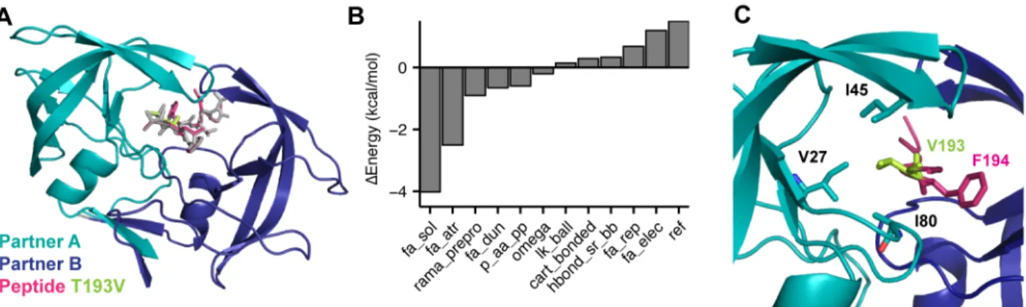
∆∆G of mutation. The first example demonstrates how Rosetta can be used to estimate and rationalize thermodynamic parameters. Here, we present an example ∆∆G of mutation calculation for the T193V mutation in the RT-RH derived peptide bound to HIV-1 protease (PDB 1kjg, Fig. 8A).103 The details of
this calculation are provided in the Supporting Information.
Figure 8: Structural model of the HIV-1 protease bound to the T4V mutant RT-RH derived peptide
(A) Structural model of the native HIV-1 peptidase (teal and dark blue), bound to the native peptide (gray) superimposed onto the T4V mutant peptide (magenta). (B) Contributions greater than + 0.1 kcal/mol to the ∆∆G of mutation for T4V. The remaining contributions are: dslf_fa13 = 0 kcal/mol, hbond_lr_bb = -0.09 kcal/mol, hbond_bb_sc = -0.05,
hbond_sc = -0.0104, fa_intra_rep = 0.01, fa_intra_sol = -0.07, and yhh_planarity = 0. (C)
Hydrophobic patch of residues surrounding position four on the RT-RH peptide.
We further investigated this result on the atomic level with the function print_atom_pair_energy_table by generating atom-pair energy tables (Supporting Information) for residues 5, 27, 45, 46, and 80 against both threonine and valine at residue 193 (Example for residue 80 in Table 3). Here, we find that the specific substitution of the polar hydroxyl on threonine with nonpolar alkyl group on valine stabilizes the peptide in the hydrophobic protease pocket. This result is consistent with chemical intuition and demonstrates how breaking down the total energies can provide insight into characteristics of the mutated structures.
Table 3: Change in atom pair energies between I80 and T4 versus V4 in kcal/mol T193→V193
Atoms
I80 Atoms
CB CG1 CG2 CD1 N 0.000 0.000 0.000 0.000 CA 0.000 0.000 0.000 0.004 C 0.000 0.000 0.000 0.008 O 0.000 0.000 0.000 -0.010 CB 0.000 0.054 0.000 -0.002 OG1 → CG1 0.008 -0.054 -0.316 -0.398 CG2 → CG2' 0.000 0.000 0.001 0.020
Protein-protein docking. The second example shows how the Rosetta energies of an ensemble of models can be used to discriminate between models and investigate the characteristics of a protein–protein interface. Below, we investigate docked models of West Nile Virus envelope protein and a neutralizing antibody (PDB 1ztx; Fig. 9A).105 Calculation details can be found in the Supporting Information.
residue in the other docking partner. The plot of energies against RMS values is called a funnel plot and is intended to mimic the funnel-like energy landscape of protein folding and binding.
Like the previous example, we decompose the energies to yield information about the nature of interactions at the interface. Here, we observed significant changes in the following energy terms upon interface formation relative to the unbound state: fa_atr, fa_rep, fa_sol, lk_ball_wtd, fa_elec, hbond_lr_bb, hbond_bb_sc, and hbond_sc (Fig. 9B). Change in the Lennard-Jones energy upon interface formation is due to the introduction of atom-atom contacts at the interface. As more atoms come into contact near the native conformation (RMS→0), the favorable, attractive energy (fa_atr) decreases whereas the unfavorable, repulsive energy (Δfa_rep) increases. Change in the isotropic solvation energy (fa_sol) is positive (unfavorable), indicating that upon interface formation, polar residues are buried. Balancing the desolvation penalty, the change in polar solvation energy (lk_ball_wtd) and electrostatics (fa_elec) is negative due to polar contacts forming at the interface. Finally, the three hydrogen bonding energies (hbond_lr_bb, hbond_bb_sc, and hbond_sc) reflect the formation of backbone–backbone, backbone–side-chain, and side-chain–side-chain hydrogen bonds at the interface.
Figure 9: Using energies to discriminate docked models of West Nile Virus and the E16 neutralizing antibody
Discussion
The Rosetta energy function represents our collaboration’s ongoing pursuit to model the rules in nature that govern biomolecular structure, stability, and association. This paper summarizes the latest version which brings together fundamental physical theories, statistical mechanical models, and observations of protein structures. This work represents almost 20 years of interdisciplinary collaboration in the Rosetta community, which in turn builds on and incorporates decades of work outside the community.
After 20 years, we have improved physical theories, structural data, representations, experiments, and computational tools; yet, energy functions are far from perfect. Compared to the first torsional potentials, energy functions are also now vastly more complex. There are countless ways to arrive at more accurate energy functions. Here, we discuss grand challenges specific to development of the Rosetta energy function in the coming decade.
Modeling biomolecules other than proteins
The Rosetta energy function was originally developed to predict and design protein structures. A clear artifact of this goal is the energy function’s dependence on statistical potentials derived from protein X-ray crystal structures. Today, the Rosetta community also pursues goals ranging from design of synthetic macromolecules to predicting interactions and structures of other biomolecules such as glycoproteins and RNA. Accordingly, an active research thrust is to generalize the all-atom energy function for all biomolecules.
Many of the physically-derived terms (e.g. van der Waals) have already been made compatible with non-canonical amino acids and non-protein biomolecules (Table S5). Recently, Bhardwaj, Mulligan & Bahl et al.67 adapted the rama_prepro, p_aa_pp, fa_dun, pro_close, omega, dslf_fa13, yhh_planarity and ref terms to be compatible with mixed-chirality peptides. Several of Rosetta’s statistical potentials are validated against quantum mechanical calculations for evaluating for non-protein models (Table 4). The first non-protein terms were added by Havranek et al.106 and Yu et al.107 who modified the hydrogen bonding potential to capture planar hydrogen bonds between protein side chains and nucleic acid bases. Renfrew et al.65,108 added molecular mechanics torsions and Lennard-Jones terms to model proteins with non-canonical amino acids, oligosaccharides, 𝛽-peptides, and oligo-peptoids.66 Labonte et al 68 implemented Woods’ CarboHydrate-Intrinsic (CHI) function109,110 which evaluates glycan geometries given the axial-equatorial character of the bonds. In addition, Das et al. added a set of terms to model Watson-Crick base pairing, 𝜋- 𝜋 interactions in base stacking, and torsional potentials important for predicting and designing RNA structures.61,111–113 These terms are presented in detail in the
Supporting Information.
Table 4: New energy terms for biomolecules other than proteins
Biomolecule Term Description Unit Ref.
Non-Canonical Amino Acids
mm_lj_intra_rep Repulsive van der Waals energy between two atoms from the same
residue
kcal/mol [65]
mm_lj_intra_atr
Attractive van der Waals energy between two atoms from the same residue
kcal/mol [65]
mm_twist Molecular mechanics derived torsion term for all proper torsions kcal/mole [65]
unfolded Energy of the unfolded state based on explicit unfolded state model AU
* [65]
split_unfolded_1b
One-body component of the two-component reference energy, lowest energy of a side chain in a dipeptide model system
AU In SI
split_unfolded_2b
Two-body component of the two-component reference energy, median two-body interaction energy based on atom type composition
AU In SI
Carbohydrates sugar_bb Energy for carbohydrate torsions kcal/mol [68]
DNA gb_elec Generalized Born model of the
electrostatics energy
kcal/mol [106]
RNA
fa_stack π-π stacking energy for RNA bases kT [112]
stack_elec Electrostatic energy for stacked RNA bases kT [113]
fa_elec_rna_phos Electrostatic energy (RNA phosphate atoms fa_elec) between kT [61]
rna_torsion Knowledge-based torsional potential for RNA
kT [61]
rna_sugar_close Penalty for opening an RNA sugar kT [61] * AU, arbitrary units
Capturing the intra- and extra-cellular environment
Rosetta traditionally models the solvent surrounding the protein using the Lazaridis-Karplus (LK) model, which assumes a solvent environment made of pure water. In contrast, biology operates under various conditions influenced by pH, redox potential, temperature, solvent viscosity, chaotropes, kosmotropes, and polarizability. Therefore, modeling more details of the intra- and extra-cellular environment would enable Rosetta to identify structures important in different biological contexts.
bilayer environment.36,60,115,116 While these improve structure prediction accuracy, both models require more computation time. This trade-off between the need for detail and computational complexity will be evaluated as Rosetta aims to model more complicated biological systems and contexts.
Table 5: Energy terms for structure prediction in different contexts
Context Term Description Unit Ref.
Membrane Environment
fa_mpsolv Solvation energy dependent on the protein orientation relative to the membrane
kcal/mol [115,1
17]
fa_mpenv
One-body membrane environment energy dependent on the protein orientation relative to the membrane
kcal/mol [115,1
17]
pH e_pH Likelihood of side chain protonation given a user-specified pH
kcal/mol [114]
The origin of energy models: top-down versus bottom-up development
Traditionally, energy functions are developed using a bottom-up approach: experimental observables serve as building blocks to parameterize physics-based formulas. The advent of powerful optimization techniques and artificial intelligence recently empowered the top-down category where numerical methods are used to derive models and/or parameters. Top-down approaches have been used to solve problems in various fields including structural biology and bioinformatics. Recently, top-down development was also applied to optimizing the Lennard-Jones, Lazaridis-Karplus, and Coulomb parameters in the Rosetta energy function (parameters in Table S4-S6).49,92
Top-down approaches have enormous potential to improve the accuracy of biomolecular modeling because more parameters can vary and the objective function can be minimized with more benchmarks. These approaches also introduce new challenges. With any computer-derived models, there is a risk of over-fitting as validation via structure prediction datasets reflect observable states, whereas simulations are intended to predict features of states that experiments cannot yet observe. Computer-derived parameters also introduce a unique kind of uncertainty. Consider the following scenario: the performance of scientific benchmarks improves as physical atomic parameters are perturbed away from the measured experimental values. As there is less physical-basis for parameters, are the predictions and interpretations still meaningful?
A highly interdisciplinary endeavor
The Rosetta energy function has advanced rapidly due to the Rosetta Community: a highly-interdisciplinary collaboration between scientists with diverse backgrounds located in over 50 labs around the world. The many facets of our team enable us to probe different aspects of the energy function. For example, expert computer scientists and applied mathematicians have implemented algorithms to speed up calculations. Dedicated software engineers maintain the code and maintain a platform for scientific benchmark testing. Physicists and chemists develop new energy terms that better model the physical rules found in nature. Structural biologists maintain a focus on created biological features and functions. We look forward to leveraging this powerful interdisciplinary scientific team as we head into the next decade of energy function advances.
Conclusion: A living energy function
For the first time since 2004,47 we have documented all of the mathematical and physical details of the Rosetta all-atom energy function highlighting the latest upgrades to both the underlying science and the speed of calculations. In addition, we illustrated how the energies can be used to analyze output models from Rosetta simulations. These advances have enabled Rosetta’s achievements in biomolecular structure prediction and design over the past fifteen years. Still, the energy function is far from complete and will continue to evolve long after this publication. Thus, we hope this document will serve as an important resource for understanding the foundational physical and mathematical concepts in the energy function. Furthermore, we hope to encourage both current and future Rosetta developers and users to understand the strengths and shortcomings of the energy function as it applies to the scientific questions they are trying to answer.
Supporting Information
Supporting Information File: RosettaEnergyFunctionReview_Alford_etal_SupportingInfo.pdf
Author Information
Corresponding Author Jeffrey J. Gray
Email: [email protected]
Department of Chemical and Biomolecular Engineering 3400 N Charles Street
Baltimore, Maryland 21218 United States Author Contributions
Wrote the manuscript: RFA, JRJ, ALF, JJG
Analysis Scripts and Examples: RFA, JRJ, MSP, JJG
Funding Sources
RFA is funded by a Hertz Foundation Fellowship and an NSF Graduate Research Fellowship. JRJ and JJG are funded by NIH GM-078221. ALF, JJG and BK are funded by NIH GM-73151. MJO is funded by NSF GM-114961. PDR and RB are funded by the Simons Foundation. MVS and RLD are funded by NIH GM-084453 and NIH GM-111819. MSP is funded by NSF BMAT 1507736. JWL is funded by NIH F32-CA189246. KK is funded by an NSF Graduate Research Fellowship and an SGF Galiban Fellowship. DB, HP and VKM are funded by NIH GM-092802. TK is funded by NIH GM-110089 and GM-117189.
Acknowledgements
References
(1) Kuhlman, B.; Baker, D. Native Protein Sequences Are close to Optimal for Their Structures. Proc. Natl. Acad. Sci. 2000, 97 (19), 10383–10388.
(2) Richardson, J. S. The Anatomy and Taxonomy of Protein Structure. Adv. Protein Chem. 1981, 34, 167–339.
(3) Leaver-Fay, A.; Tyka, M.; Lewis, S. M.; Lange, O. F.; Thompson, J.; Jacak, R.; Kaufman, K. W.; Renfrew, P. D.; Smith, C. A.; Sheffler, W.; Davis, I. W.; Cooper, S.; Treuille, A.; Mandell, D. J.; Richter, F.; Ban, Y.-E. A.; Fleishman, S. J.; Corn, J. E.; Kim, D. E.; Lyskov, S.; Berrondo, M.; Mentzer, S.; Popović, Z.; Havranek, J. J.; Karanicolas, J.; Das, R.; Meiler, J.; Kortemme, T.; Gray, J. J.; Kuhlman, B.; Baker, D.; Bradley, P. Rosetta3: An Object-Oriented Software Suite for the Simulation and Design of Macromolecules. Methods Enzymol. 2011, Volume 487, 545–574. (4) Anfinsen, C. B. Principles That Govern the Folding of Protein Chains. Science 1973, 181 (4096),
223–230.
(5) Lennard-Jones, J. On the Determination of Molecular Fields I: From the Variation of Viscosity of a Gas with Temperature. R. Soc. London, Ser. A, Contain. Pap. a Math. Phys. Character 1924, 106, 441–462.
(6) Lennard-Jones, J. On the Determination of Molecular Fields II: From the Variation of Viscosity of a Gas with Temperature. R. Soc. London, Ser. A, Contain. Pap. a Math. Phys. Character 1924, 106, 464–477.
(7) Levitt, M.; Lifson, S. Refinement of Protein Conformations Using a Macromolecular Energy Minimization Procedure. J. Mol. Biol. 1969, 46 (2), 269–279.
(8) Urey, H. C.; Bradley, C. A. The Vibrations of Pentatonic Tetrahedral Molecules. Phys. Rev. 1931, 38 (11), 1969–1978.
(9) Westheimer, F. . Calculation of the Magnitude of Steric Effects. Steric Eff. Org. Chem. 1956, 523– 555.
(10) Lifson, S.; Warshel, A. Consistent Force Field for Calculations of Conformations, Vibrational Spectra, and Enthalpies of Cycloalkane and N-Alkane Molecules. J. Chem. Phys. 1968, 49 (11), 5116.
(11) Warshel, A.; Lifson, S. Consistent Force Field Calculations. II. Crystal Structures, Sublimation Energies, Molecular and Lattice Vibrations, Molecular Conformations, and Enthalpies of Alkanes. J. Chem. Phys. 1970, 53 (2), 582.
(12) Levitt, M. Energy Refinement of Hen Egg-White Lysozyme. J. Mol. Biol. 1974, 82 (3), 393–420. (13) Gelin, B. R.; Karplus, M. Sidechain Torsional Potentials and Motion of Amino Acids in Porteins:
Bovine Pancreatic Trypsin Inhibitor. Proc. Natl. Acad. Sci. U. S. A. 1975, 72 (6), 2002–2006. (14) Levinthal, C.; Wodak, S. J.; Kahn, P.; Dadivanian, A. K. Hemoglobin Interaction in Sickle Cell
Fibers. I: Theoretical Approaches to the Molecular Contacts. Proc. Natl. Acad. Sci. U. S. A. 1975, 72 (4), 1330–1334.
(15) Cornell, W. D.; Cieplak, P.; Bayly, C. I.; Gould, I. R.; Merz, K. M.; Ferguson, D. M.; Spellmeyer, D. C.; Fox, T.; Caldwell, J. W.; Kollman, P. A. A Second Generation Force Field for the Simulation of Proteins, Nucleic Acids, and Organic Molecules. J. Am. Chem. Soc. 1996, 118 (9), 2309–2309. (16) Mayo, S. L.; Olafson, B. D.; Goddard, W. A. DREIDING: A Generic Force Field for Molecular
Simulations. J. Phys. Chem. 1990, 94 (26), 8897–8909.