Valerie Johanne Langlois
A thesis submitted to the faculty at the University of North Carolina at Chapel Hill in partial fulfillment of the requirements for the degree of Doctor of Philosophy in the
Department of Psychology & Neuroscience.
Chapel Hill 2019
ii © 2019
iii
ABSTRACT
Valerie Johanne Langlois: Does experience change the informativity of disfluency as a marker of information status?
(Under the direction of Jennifer Arnold)
iv
ACKNOWLEDGEMENTS
v
TABLE OF CONTENTS
LIST OF TABLES ... vii
LIST OF FIGURES ... viii
INTRODUCTION ... 1
Background ... 2
Inferences from disfluency ... 3
Changes to informativity ... 6
The current study... 11
EXPERIMENT 1 ... 15
Methods ... 15
Participants ... 15
Materials ... 15
Procedure... 17
Eye-movement recording ... 19
Analytic approach ... 19
Results ... 21
Target word time window ... 21
Disfluency time window ... 23
Experiment 1 Discussion ... 25
EXPERIMENT 2 ... 26
vi
Participants ... 26
Materials ... 26
Procedure... 27
Analytic approach ... 27
Results ... 27
Target word time window ... 28
Trial order ... 29
Disfluency time window ... 30
Experiment 2 Discussion ... 32
GENERAL DISCUSSION ... 33
APPENDIX: ADDITIONAL FIGURES ... 37
vii
LIST OF TABLES
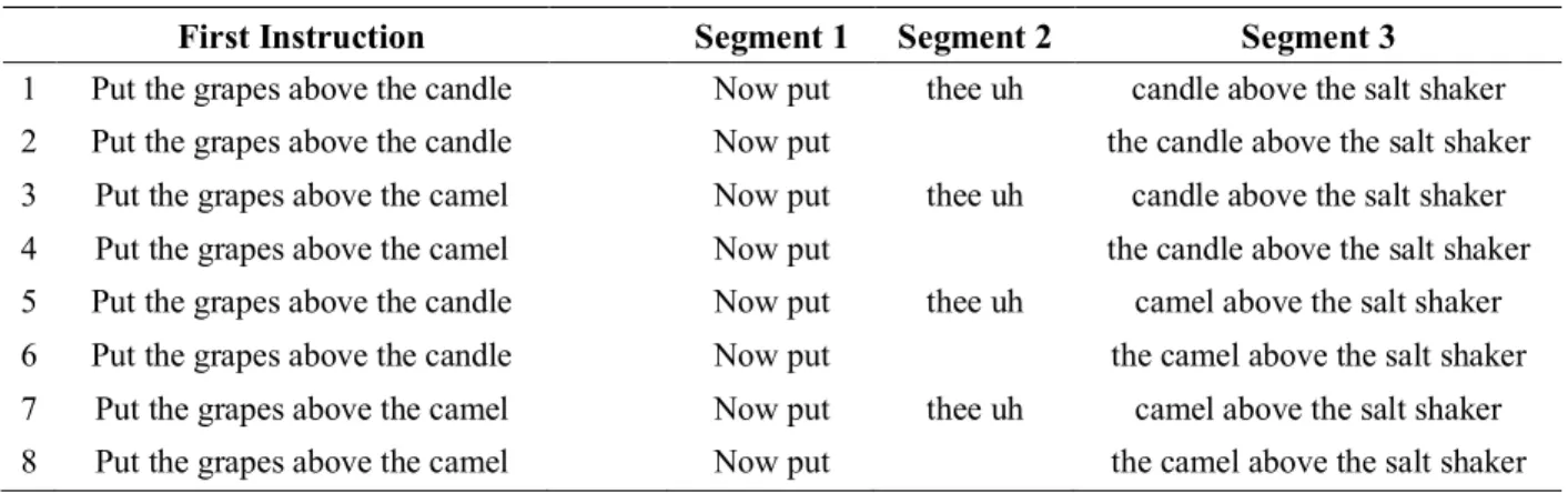
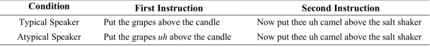
Table 1. First and second instructions for an item ... 16
Table 2. Example of a filler trial ... 17
Table 3. Output from Experiment 1 statistical models in both time windows ... 24
Table 4. Example of an item comparing the two speaker conditions ... 26
viii
LIST OF FIGURES
Figure 1. Example of a critical trial ... 12 Figure 2. Order of trials in each experiment ... 14 Figure 3. Experiment 1 average percentage of looks for disfluent and
fluent trials, grouped by speaker condition... 22 Figure 4. Experiment 1 interaction between disfluency and target status ... 22 Figure 5. Experiment 1 average looks across time for disfluent and
fluent trials separated by speaker condition ... 23 Figure 6. Experiment 1 timecourse of average looks (left) and average
looks (right) to the two discourse-given objects during the
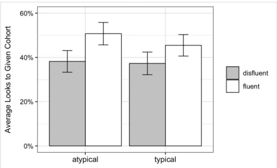
disfluency time window... 24 Figure 7. Experiment 2 average percentage of looks for disfluent
and fluent trials, grouped by speaker condition ... 28 Figure 8. Experiment 1 average looks across time for disfluent and
fluent trials separated by speaker condition ... 29 Figure 9. Average percentage of looks to the given cohort over the
course of Experiment 2 in fluent and disfluent conditions across
the two speaker conditions... 30 Figure 10. Experiment 2 timecourse of average looks (left) and average
looks (right) to the two discourse-given objects during the
1
INTRODUCTION
Disfluency, such as uhs and ums, occur frequently in natural conversation. These disruptions in speech can lead listeners to infer that the speaker is having production difficulty, and anticipate reference to something discourse new (Arnold, Tanenhaus, Altmann, & Fagnano, 2004) or unfamiliar (Arnold, Kam, & Tanenhaus, 2007; Barr, 2001), unpredictable (Corley, MacGregor, & Donaldson, 2007), or anticipate likely repair words (Lowder & Ferreira, 2016). Listeners can use disfluency as a signal to narrow down their expectations, making it
informative. However, this raises questions about how exposure to the distribution of disfluency is related to inferences listeners draw about production difficulty. Recent evidence has shown that this disfluency effect disappears when listeners thought they were hearing speech from an atypical speaker, e.g. someone with object agnosia, a stutterer, or a non-native speaker (Arnold et al., 2007; Bosker, Quené, Sanders, & de Jong, 2014; Lowder, Maxfield, & Ferreira, 2016). These findings indicate that the informativity of disfluency is modulated by assumptions about the speaker. However, it is unclear whether listeners could have based their assumptions about cognitive ability on exposure to the distribution of disfluency.
This study investigates whether the distribution or frequency of filler words (e.g. uhs and ums) can change the informativity of disfluency as a signal to discourse status. In the following sections, I provide a broad overview of speech disfluency, its role as a signal to planning
2
manipulated (Experiment 1) and the frequency of disfluency is increased (Experiment 2). These questions are broadly related to questions about how statistical information in language is used, and how a change in distribution can change the informativity of a cue, like disfluency.
Background
While conversation is thought to be a continuous speech stream, it is actually filled with disruptions and delays. Regardless, speech is surprisingly easy to understand. Listeners are still able to comprehend the meaning of the message, even one filled with uhs and ums. These filler words (e.g. uhs and ums) are a type of speech disfluency, which encompasses a large category consisting of not only filler words, but also silent pauses, prolonged vowels, repeated words, and speech errors or repairs. Despite the listener’s understanding of the communicative message, speakers nevertheless continue to strive for fluent speech.
Listeners are frequently exposed to disfluency in speech. Around 2 to 26 disfluencies occur for every 100 words, with the number varying depending on the inclusion or exclusion of silent pauses (Fox Tree, 1995). When looking across the distribution of disfluency, speakers tend to be disfluent as a result of difficulty in planning (Bell et al., 2003; Clark & Fox Tree, 2002; Clark & Wasow, 1998; Fox Tree & Clark, 1997), such as trouble with word retrieval or grammatical structure. As a result, the distribution of disfluency is systematic across
conversation (Maclay & Osgood, 1959; Shriberg, 1996). Disfluency is more likely to occur prior to utterances that reflect a difficulty in formulation.
3
discourse-new objects (21%) compared to given objects (16%) in sentences containing either a 1 to 2-word noun phrase or a complex description. Not only does this suggest that the
inaccessibility of new information leads to difficulty in planning, but also that there is a link between discourse status and the distribution of disfluency. Speakers tend to be more disfluent before discourse-new information relative to given information.
Inferences from disfluency
When a speaker is disfluent, listeners can infer that a speaker is having some sort of difficulty with lexical retrieval. Arnold et al. (2004) presented participants with instructions to move objects around on a screen that were either previously mentioned or new to the discourse. Two out of the four objects on the screen had phonologically similar names (e.g. candle and camel), and were cohort competitors, while the other objects were phonologically dissimilar distractors. Participants followed auditory instructions such as Put the grapes above the candle. Now put {thee uh/the}… which was followed by one of the two cohort competitors, either candle or camel. To address listener interpretation following the disfluency, eye-tracking was used to analyze fixations to cohort competitors during the window of the temporary ambiguity (candle vs. camel). Previous work suggests that listeners begin to fixate on an image matching the given input about 200ms after the onset of a spoken word (Allopenna, Magnuson, & Tanenhaus, 1998; Tanenhaus, Spivey-Knowlton, Eberhard, & Sedivy, 1995). The timecourse of the eye movements is also closely time locked to the referring input (Eberhard, Spivey-Knowlton, Sedivy, &
4
communicative signal is informative; it allows the listener to predict an upcoming referent, even before the speaker finishes the utterance.
This disfluency bias is not limited to only discourse-new information. Rather than a direct association between disfluency and discourse-new information, this bias has been shown in conjunction with other types of difficulty. For example, listeners can use disfluency as a cue to anticipate reference to something unfamiliar or novel, such as an abstract symbol or object (Arnold et al., 2007). Similarly, Corley, MacGregor, & Donaldson (2007) found a reduced N400 effect for unpredictable words following a disfluency compared to fluent speech, which reflects an ease of processing and integrating those words into the context. Watanabe, Hirose, Den, & Minematsu (2008) showed that listeners also expect reference to complex shapes following a filled pause, as reflected by faster response times. Furthermore, listeners can use repair
disfluencies (e.g. uh I mean) to anticipate an upcoming reparandum (Lowder & Ferreira, 2016). Lastly, even the confidence of the speaker can affect listener’s comprehension (Barr, 2001).
5
had no other disambiguating lexical information besides the adjective. Between the two same colored objects, they were more likely to choose the unfamiliar object over the familiar one in a trial where disfluency occurred before the color adjective. They also tended to look towards the unfamiliar object after the onset of the color word in the same trial. Similar to Arnold et al. (2004), listeners in this task inferred that disfluency signals a difficulty in planning; speakers are probably having more trouble lexically retrieving the name of the unfamiliar object, which leads to disfluency. However, when participants were explicitly told that the speaker had object agnosia (trouble naming objects), the disfluency bias disappeared (Arnold et al., 2007), which suggests the possibility that participants inferred that the agnosic speaker had difficulty naming either object, regardless of its familiarity. Therefore, disfluency no longer acted as a cue to unfamiliar referents, in contrast to their previous experiment without the description of the agnosic speaker. In other words, disfluency became less informative. When disfluency is attributed to the characteristics of the agnosic speaker, listeners are less likely to use disfluency to anticipate upcoming information.
6
Changes to informativity
This line of research suggests that disfluency is less informative to the listener once it is attributed to something else, e.g. stuttering, language proficiency, or agnosia, and that the effect of disfluency is malleable. However, this raises the question of other ways this effect can change. Does the effect change solely due to assumptions about the speaker, where disfluency is
attributed to a speaker’s cognitive state? Alternatively, could a change in the statistics of
7
changes over the course of the experiment, which is only a short period of time when compared to the lifetime experience a listener typically has of modifiers.
This concept of “informativeness” is not limited to the word level. The informative use of prosody has also been manipulated in a similar manner. In the sentence Tap the frog with the flower, there are two possible interpretations: 1) Using the flower to tap the frog, or 2) tapping the frog who has a flower in its possession. Speakers can use the location of the prosodic
boundary to disambiguate between the two interpretations, where Tap % the frog with the flower indicates with the flower is a modifier of the frog and Tap the frog % with the flower specifies the flower as an instrument. This prosodic information is used by listeners for syntactic
interpretation, and also to anticipate upcoming information (Kraljic & Brennan, 2005; Schafer, Speer, Warren, & White, 2000; Snedeker & Trueswell, 2003). However, when the speaker unreliably uses prosody, listeners no longer use prosodic information to predict upcoming material (Nakamura, Harris, & Jun, 2018). Prosody becomes less informative, and listeners must rely on other cues instead.
Language use has also been influenced by exposure on the syntactic level. When speakers are exposed to double-object dative sentences such as The corrupt inspector offered the bar owner a deal to describe pictured events, they later produced this same structure but generalized to new events (e.g. The boy is handing the girl a valentine) (Bock, 1986). Exposure to this specific syntactic structure has been shown to last over a long period of time in production (Bock & Griffin, 2000; Chang, Dell, Bock, & Griffin, 2000). It changes the extent to which the speaker uses the double-object dative structure. Computational models further support this claim,
8
what) and uses it to predict upcoming words. By learning from the errors made in prediction (e.g. the word predicted from context did not occur), the model is able to adjust to these changes. What results is a model acquiring these syntactic structures over time. This also transfers over to comprehension, where recently primed structures have been shown to shape expectations about upcoming syntactic structures (Thothathiri & Snedeker, 2008). Participants primed with the double-object dative (e.g. Show the horse the book) rather than the prepositional object dative (e.g. Show the horn to the dog) fixated more on the animate referent over the inanimate one during the temporary ambiguity window. Furthermore, these predictions are modified based on the error signal of the previous input (Fine & Jaeger, 2013). When listeners predict the wrong referent before the disambiguating information, the wrong prediction results in self-adjustment, consistent with Chang et al. (2006). Over time, the listener adapts to the exposure, and learns to expect certain structures over others.
Previous studies on modification and prosody showed that even with short-term exposure to a novel distribution, comprehenders’ behavior suggested that they perceived these cues as less informative (Grodner & Sedivy, 2011; Nakamura et al. 2018). In addition,
expectations about syntactic structures can change over time through exposure (Thothathiri & Snedeker, 2008). These studies support the idea that when the distribution goes against listeners’ expectations, listeners adjust their reliance on these cues. This suggests the possibility that perhaps this will extend to discourse processing. Based on previous studies (e.g. Grodner & Sedivy, 2011; Nakamura et al. 2018), disfluency may become less informative if disfluency occurs in unexpected places, such as in (1).
9
In (1), the placement of disfluency is right before a given noun (candle), which is in an
unexpected location. Speakers are usually not disfluent before something previously mentioned. The distribution of disfluency is systematic, with disfluency more likely to occur as a result of planning difficulty (Bell et al., 2003; Clark & Fox Tree, 2002; Clark & Wasow, 1998; Fox Tree & Clark, 1997). Why would a speaker have difficulty with a word mentioned in a recent
utterance? When disfluency occurs before already mentioned information, it goes against the systematic distribution listeners may be expecting. If a listener continues to hear disfluency in unexpected places like in (1), it creates a novel distribution of disfluency. This distribution may go against the listener’s lifetime experience with disfluency, as discourse-new information tends to follow disfluency rather than discourse-given information.
The frequency of disfluency might also affect its informativity to listeners. For example, a speaker may be frequently disfluent, as in (2).
10
Alternatively, previous work does not negate the idea that changing the frequency of disfluency could also change the disfluency bias. For example, Lowder et al. (2016) exposed their participants to stutterer speech; each sentence in the stutterer condition included one or two instances of stuttering while this was not the case for the non-stutterer speaker. Therefore, perhaps the attenuation of the disfluency bias was brought on by the mere frequency of disfluency. In addition, disfluency focuses listeners’ attention on speech (Collard, Corley, MacGregor, & Donaldson, 2008; Fox Tree, 2001; Fraundorf & Watson, 2011). If listeners are exposed to frequent disfluency, it is possible that disfluency becomes less salient compared to if it only occurred occasionally. This view predicts that if listeners hear disfluency too frequently, they may stop paying attention to it, leading to disfluency becoming less informative.
The current study investigates whether changes to listener comprehension arise based on two different distributions of disfluency: 1) a novel distribution where disfluency is always in unexpected locations and 2) an expected distribution where disfluency overall occurs more frequently, but always in expected locations. I hypothesized that listeners exposed to a novel distribution may learn that disfluency does not precede unmentioned information. I predicted that in this condition, disfluency may become less informative to the listener. They may be less likely to use disfluency to anticipate upcoming discourse-new information. On the other hand, if
disfluency occurs frequently but still in expected places, listeners have no reason to believe that the correlation between disfluency and discourse-new information is affected. Therefore,
11
The current study
The current study consists of two experiments that test whether disfluency becomes less informative when listeners are exposed to either a novel distribution of disfluency or an overall increase in disfluency. The stimuli were designed for the purpose of seeing whether listeners change their behavior in response to the new distribution or frequency of disfluency. It is possible that listeners may make higher-level inferences about the characteristics of a speaker based on the manipulation. Therefore, I ask two questions in this project. First, if a speaker is consistently disfluent in unexpected places, such as before previously mentioned information, will the disfluency cue still be informative to the listener (novel distribution)? Second, if a speaker is frequently disfluent, but before discourse-new information as expected, will disfluency continue to benefit listeners (frequent disfluency)?
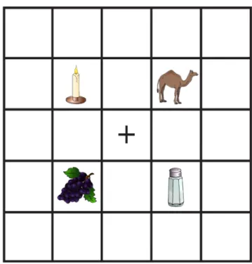
The study used a paradigm similar to Arnold et al. (2004), where trials varied by fluency (fluent or disfluent) and the discourse status of the target cohort (given or discourse-new). In each trial, participants followed a set of spoken instructions and moved objects around on the screen while their eye movements were tracked (Figure 1). The first sentence mentioned one of the cohorts from a pair (e.g. either candle or camel), establishing it as the given object. The second sentence contained the critical target expression, where participants either heard the given referent (e.g. candle) or the discourse-new referent (e.g. camel). The second sentence was either fluent or disfluent before the critical target.
First Instruction: Put the grapes above the candle.
Second Instruction:
12
Disfluent/Given: Now put thee uh candle above the salt. Disfluent/New: Now put thee uh camel above the salt.
Figure 1. Example of a critical trial
The other two objects were distractors unrelated to the cohort pairs (e.g. grapes, salt). The onset of each cohort pair were phonologically similar, which allowed for competition between the two words.
13
speaker, discourse-new information followed disfluency for the disfluent filler trials. Importantly, across speaker conditions, the amount of disfluency stays constant. Half of the fillers in both conditions were disfluent, but differ in location.
Atypical speaker: Put the tomato in the space to the right of the knife. Now put the bow above thee uh tomato.
Typical speaker: Put the tomato in the space to the right of the knife. Now put thee uh bow above the tomato.
Experiment 2 manipulated the frequency of disfluency. As with Experiment 1, There was an atypical speaker and a typical speaker. However, the atypical speaker was twice as disfluent than the typical speaker.
Atypical speaker: Put the tomato um uh in the space to the right of the knife. Now put the thee uh bow above tomato.
Typical speaker: Put the tomato in the space to the right of the knife. Now put thee uh bow above the tomato.
14
Figure 2. Order of trials in each experiment. Participants received eight filler trials depending on the speaker condition in the beginning of the task.
In summary, both experiments were a 2 by 2 by 2 design. Similar to Arnold et al. (2004), eye-tracking was used as a more sensitive, on-line measure of listener interpretation. The
between-subjects condition varied by speaker (atypical vs. typical), and the within-subjects condition varied by fluent or disfluent trials, and also given or discourse-new. This design allowed me to investigate the disfluency effect across the two different speakers.
15
EXPERIMENT 1
Methods
Participants
50 participants were recruited from the UNC undergraduate participant pool: 25 in the typical condition and 25 in the atypical condition. All participants were native speakers of English and received class credit in compensation.
Materials
Stimuli included 68 trials consisting of 24 critical trials and 44 filler trials. Each trial consisted of a visual display and an accompanying set of instructions. The visual display was composed of four objects within a 5 by 5 grid (Figure 1): two cohort competitors and two distractors. Pairs of cohort competitors were chosen based on the phonological similarity between the first syllable of the two object labels, consistent with Arnold et al. (2004). The distractors did not share this same phonological overlap with the cohort competitors. Images of the objects were in color and obtained from Rossion & Pourtois (2010), adapted from Snodgrass & Vanderwart (1980).
16
which eliminated the possibility of prosody being used as a signal for any upcoming disfluency. In addition, the same audio recording of the disfluency marker thee uh (Segment 2) was used within an item, as was the segment after the disfluency depending on condition (Segment 3).
Table 1. First and second instructions for an item.
First Instruction Segment 1 Segment 2 Segment 3
1 Put the grapes above the candle Now put thee uh candle above the salt shaker 2 Put the grapes above the candle Now put the candle above the salt shaker 3 Put the grapes above the camel Now put thee uh candle above the salt shaker 4 Put the grapes above the camel Now put the candle above the salt shaker 5 Put the grapes above the candle Now put thee uh camel above the salt shaker 6 Put the grapes above the candle Now put the camel above the salt shaker 7 Put the grapes above the camel Now put thee uh camel above the salt shaker 8 Put the grapes above the camel Now put the camel above the salt shaker
Cross-splicing only occurred within an item, and not across all items (e.g. the same audio recording for Now put is not the same for every trial). There was also no cross-splicing in any of the filler trials.
Both discourse status and disfluency of the instruction were within-item manipulations, resulting in 8 different lists within each speaker condition. Across the lists, cohort competitors were matched in frequency, visual complexity, and familiarity. The two cohort competitors were always initially positioned in either the top or bottom row. Locations of the cohort competitors were counterbalanced within a list: the given cohort appeared equally in each of the four
locations, and the target cohort competitor, the cohort that the participant is instructed to move, appeared equally in each of the four locations.
17
objects was always re-mentioned in the second instruction, and varied between the first mention or the second mention from the first instruction. The mentioned object appeared in either the grammatical object position or the object position of the prepositional phrase in the second instruction (22 of each). For filler trials in the atypical speaker condition, the speaker was
disfluent before the mentioned object. The only difference between the two speaker conditions in Experiment 1 was the location of the disfluency; before the discourse-new object (typical) or before the given object (atypical) (Table 2).
Table 2. Example of a filler trial.
Condition First Instruction Second Instruction
Typical Speaker Put the ring to the right of the bed Now put thee uh bell above the ring Put the cake to the right of the peach Now put the peach below thee uh lettuce Atypical Speaker Put the ring to the right of the bed Now put the bell above thee uh ring
Put the cake to the right of the peach Now put thee uh peach below the lettuce
Procedure
Participants wore a head-mounted eye-tracker (SR Research Eyelink II eye-tracker). They completed a 9-point calibration and validation procedure before the start of the task. After calibration, participants were told that the task involved listening to sets of spoken instructions and using the mouse to move objects around on the screen as instructed. After the initial instructions, participants completed three practice trials. The practice trials were similar to the experimental trials within the speaker condition in order to further establish the manipulation. After participants completed the practice trials, they moved on to the experimental task.
18
resulting in 16 lists total. Lists were counterbalanced, allowing for equal numbers of disfluent and fluent trials, and mention of a given or discourse-new object in the second instruction. All participants completed the same 44 filler trials, though these trials varied based on differences in speaker condition. Participants were presented with 68 trials that each have two instructions. Eight of the filler trials were presented first in pseudorandom order to expose the participant to the manipulation before the critical trials. The rest of the filler and critical trials followed afterwards and were pseudorandomized.
Before the onset of each trial, a drift-check was performed to correct for any small head movements made by the participant. Participants looked at a small black and white dot presented at the center of the screen while pressing the spacebar. In the unlikely event that the participant did not pass drift-check, the experimenter stopped the task for re-calibration.
19
Eye-movement recording
Eye-movements were recorded using a SR Research Eyelink II, head-mounted eye-tracker at a sampling rate of 250 Hz. Samples were categorized as saccades or fixations as determined by the default settings of the Eyelink II system.
Analytic approach
Samples during the second instruction of the critical trials were analyzed in two time windows: 200ms from the onset of the disfluency for a duration of 600ms, and 200ms from the onset of the target word for a duration of 400ms. The timing of the target word window was the same as in Arnold et al. (2004). In addition, both of these windows were decided by an earlier pilot study. Fixations and saccades were included together in analyses to represent “looks” to an object.
Following Arnold et al. (2004), “looks” to each interest area were calculated for each trial by collapsing saccades and fixations across each window. However, there is a slight difference between Arnold et al. (2004) and the current study in how saccades are included in the analyses, due to a difference in software. In Arnold et al. (2004), if a saccade occurred prior to a fixation, the entire saccade was grouped with that fixation to form a “look”. In the current study, only a proportion of the saccade that fell in an interest area during the specified time window was included.
Two dependent variables were calculated. For my primary analysis I examined the preference for looking at the given cohort over the new cohort. For this analysis, I calculated the empirical logit of the given cohort, using empirical logit transformation, based on Barr (2008):
20
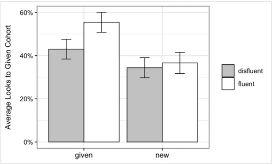
As a secondary analysis, I tested whether participants made predictions in response to the disfluency by shifting attention more to the new vs. given objects during the disfluency window. To test this, looks to all given objects were transformed using the same formula. Instead of cohorts, objects were separated into given and new objects.
𝐿𝑁 # 𝑆𝑢𝑚 𝑜𝑓 𝑙𝑜𝑜𝑘𝑠 𝑡𝑜 𝑔𝑖𝑣𝑒𝑛 𝑜𝑏𝑗𝑒𝑐𝑡𝑠 + 0.5
𝑇𝑜𝑡𝑎𝑙 𝑠𝑢𝑚 𝑜𝑓 𝑙𝑜𝑜𝑘𝑠 𝑡𝑜 𝑎𝑙𝑙 𝑜𝑏𝑗𝑒𝑐𝑡𝑠 − 𝑆𝑢𝑚 𝑜𝑓 𝑙𝑜𝑜𝑘𝑠 𝑡𝑜 𝑔𝑖𝑣𝑒𝑛 𝑜𝑏𝑗𝑒𝑐𝑡𝑠 + 0.5 >
SAS 9.4 Proc Mixed was used to analyze the empirical logit of looks from both time windows. Models of each dependent variable included random intercepts of both participant and item to account for nesting. Random slopes of the primary predictors were also included by participant and by item only if appropriate.
21
Results
48 participants were included in the following analyses. Two participants were excluded due to technical difficulties. Trials were excluded if the total sum of all looks was less than 25% of the total possible number of looks in that time window. For the primary analysis in the target word time window, trials were excluded if there were no looks to either of the two cohort competitors. In total, 155 observations were excluded from the final analysis during the target word window, with 995 observations remaining. Exclusion criteria remained the same for the secondary analysis during the disfluency time window, however only disfluent trials were included. Trials were also excluded if there were no looks to any of the four objects, resulting in a total of 543 observations.
Target word time window
To test the question of whether there was a disfluency effect in either of the two speaker conditions, I analyzed eye movement data during the target word window. As shown in Figure 2, participants were more likely to fixate on the given cohort in the fluent condition relative to the disfluent condition. This pattern emerged as a main effect of disfluency in the statistical analysis, indicating that there was an overall disfluency effect in both speaker conditions. There was also a significant main effect of target status, since the dependent measure was looks to the given cohort. There were more looks to the given cohort when the given cohort was the target.
22
compared to when the given cohort was the competitor (see Figure 4). See Table 3 for model output and Figure 5 for average looks across the course of the trial.
Figure 3. Experiment 1 average percentage of looks for disfluent and fluent trials, grouped by speaker condition. Error bars represent 95% within-subject confidence intervals.
23
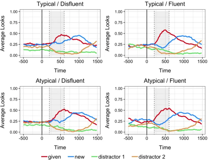
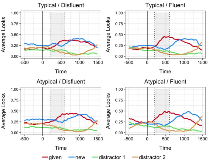
Figure 5. Experiment 1 average looks across time for disfluent and fluent trials separated by speaker condition.
Disfluency time window
24
of speaker condition within this time window. Looks to the discourse-given objects during the disfluency period did not differ across the two different conditions (see Figure 6).
Figure 6. Left: Timecourse of average looks to the two discourse-given objects during the disfluency time window. Shaded region represents the window of interest. Right: Average looks across speaker condition.
Table 3. Output from Experiment 1 statistical models in both time windows
Target Time Window
Model Parameters Estimate SE t p
Order .000 .007 -.070 .948
Speaker Condition .132 .258 .510 .608
Disfluent vs. Fluent -.518 .224 -2.310 .021
Target Status 2.022 .462 4.380 < .0001
25
Speaker Condition*Disfluent .493 .450 1.100 .273
Speaker Condition*Target Status -.179 .493 -.360 .717
Speaker Condition*Target Status*Disfluent -1.099 .897 -1.220 .221
Disfluency Time Window
Model Parameters Estimate SE t p
Speaker Condition .029 .536 .050 .957
Target Status .482 .364 1.320 .186
Speaker Condition*Target Status .542 .728 .740 .457
All predictors were grand-mean centered. The reference condition for Speaker condition is typical. Reference
condition for Disfluent vs. Fluent is Disfluent. Reference condition for Target Status is given.
Experiment 1 Discussion
The goal of Experiment 1 was to investigate whether a novel distribution of disfluency affects its informativity as a signal to discourse-given information. I predicted that if a speaker is frequently disfluent in unexpected places, listeners should have no reason to infer that the
speaker is having difficulty with planning. As a consequence, the disfluency effect in the atypical speaker condition should be attenuated. However, the results from Experiment 1 indicate that there is no difference in the disfluency effect across the two speaker conditions. In both speaker conditions, listeners continued to use disfluency informatively.
26
EXPERIMENT 2
Methods
Participants
55 participants were recruited from the UNC undergraduate participant pool: 27 in the typical condition and 28 in the atypical condition. All participants were native speakers of English, and received class credit in compensation.
Materials
Visual stimuli were the same as Experiment 1. The only changes from Experiment 1 were the recorded instructions. As with Experiment 1, participants heard two instructions through a set of computer speakers for each trial. For all items in the atypical speaker condition, the speaker was always disfluent in the first instruction, resulting in a much higher rate of disfluency (100% of trials). The typical speaker condition was the same as in Experiment 1, with disfluency occurring in only 50% of the trials. In both speaker conditions, disfluency occurred in natural locations. The second instruction was the same for both conditions: either the cohort from the first instruction (given) or the second cohort (new) was mentioned. The same recordings from Experiment 1 for the second instruction were used for the current experiment (see Table 4).
Table 4. Example of an item comparing the two speaker conditions.
Condition First Instruction Second Instruction
27
Unlike Experiment 1, filler trials in the current experiment did not differ between the two speaker conditions. In both speaker conditions, the speaker was always disfluent before the unmentioned object in half of the filler trials. The filler trials followed the same structure as the fillers in the typical speaker condition from Experiment 1 and used the same audio recordings.
Procedure
The procedure was exactly the same as Experiment 1.
Analytic approach
As in Experiment 1, SAS 9.4 Proc Mixed was used to analyze the empirical logit of looks to the given cohort during the Target Word window, and the empirical logit of looks to the given objects during the disfluency window. Primary predictors were the same as Experiment 1
(speaker condition, disfluent vs. fluent, and target status). Trial order was also included in the model. Models of each dependent variable included random intercepts of both participant and item to account for nesting, and random slopes of the primary predictors were included by participant and by item if appropriate. In addition to the primary predictors, all two-way and three-way interactions were added to the model. For the disfluency window, only disfluent trials were included in the model.
Results
28
disfluency time window, only disfluent trials were included, resulting in a total of 557 observations.
Target word time window
The same question was tested as in Experiment 1: Does the disfluency effect change across the two speaker conditions? Eye movement data were analyzed during the target word window. As shown in Figure 7, participants looked more at the given cohort in fluent trials relative to disfluent trials. This pattern emerged as a significant main effect of disfluency in the statistical analysis. There was an overall significant main effect of target status; participants looked more at the given cohort when it was discourse-given. As with Experiment 1, the
interaction between speaker condition and disfluency is not significant, indicating no differences between the two speaker conditions. See Table 5 for model output and Figure 8 for timecourses.
29
Figure 8. Experiment 2 average looks across time for disfluent and fluent trials separated by speaker condition.
Trial order. Unlike in Experiment 1, the order of the trials did have a marginally
30
between order, disfluency, and speaker condition was not significant, which means that the disfluency effect did not change over time in either of the two speaker conditions.
Figure 9. Average percentage of looks to the given cohort over the course of the experiment in fluent and disfluent conditions across the two speaker conditions.
Disfluency time window
31
speaker conditions. Only disfluent trials were included in this analysis. Since I did not find an effect of speaker on the disfluency bias during the target time window, I expected to not find an effect in the disfluency time window. As with Experiment 1, there was neither a main effect of speaker condition nor a main effect of discourse status. In addition, the interaction was not significant (Figure 10). See Table 5 for model output.
Figure 10. Left: Timecourse of average looks to the two discourse-given objects during the disfluency time window. Shaded region represents the window of interest. Right: Average looks across speaker condition.
Table 5. Output from Experiment 2 statistical models in both time windows
Target Time Window
32
Order -.012 .007 -1.770 .077
Speaker Condition .297 .338 .880 .380
Disfluent vs. Fluent -1.227 .236 -5.210 < .0001
Target Status 1.622 .389 4.170 < .0001
Disfluent*Target Status .070 .471 .150 .883
Speaker Condition*Disfluent -.023 .471 -.050 .962
Speaker Condition*Target Status .405 .593 .680 .495
Speaker Condition*Target Status*Disfluent -.091 .943 -.100 .923
Order*Speaker Condition .036 .014 2.650 .008
Order*Disfluent -.002 .014 -.11 .913
Order*Condition*Disfluent .033 .028 1.17 .244
Disfluency Time Window
Model Parameters Estimate SE t p
Speaker Condition .275 .668 .410 .681
Target Status .053 .355 .150 .880
Speaker Condition*Target Status -.348 .711 -.490 .625
All predictors were grand-mean centered. The reference condition for Speaker condition is typical. Reference
condition for Disfluent vs. Fluent is Disfluent. Reference condition for Discourse Status is given.
Experiment 2 Discussion
33
GENERAL DISCUSSION
The current study tested whether either a novel distribution or an increase in frequency could change the way listeners used disfluency to guide interpretation. In Experiment 1, though the atypical speaker was always disfluent before discourse-given referents, this novel distribution did not affect listener biases for discourse-new referents. In Experiment 2, an overall increase in disfluency did not change listeners’ interpretation.
These results have two possible interpretations. Perhaps changing the distribution of disfluency does affect interpretation, but Experiment 1 failed to show any evidence of a change in its informativity. It is possible that participants did not have enough exposure to override a lifetime experience with disfluency preceding discourse-new information. However, Grodner & Sedivy, (2011) were able to change the informativity of modifiers with only 26 filler trials, which raises the question of whether there is something different about disfluency. Perhaps since it is a subtler cue, listeners may need more than one experimental session to adapt to it.
34
listening to during the task. Therefore, if participants did make any sort of assumptions about the speaker in the current study, it was based only on distributional information. Based on the results of the current study, however, it is unknown whether listeners made any inferences about the speaker at all.
More recent work has investigated the same questions as the current study, but in the context of low-frequency referents instead of discourse-new referents (Bosker, van Os, Does, & van Bergen, 2019). Listeners exposed to a native speaker and an atypical distribution of
disfluency learned to anticipate high-frequency referents following a disfluency. In contrast, listeners did not adapt to a novel distribution of disfluency when the speaker was clearly non-native. Again, this raises questions about the mechanisms underlying disfluency. Listeners can adapt to speakers who use both modifiers and prosody uninformatively (Grodner & Sedivy, 2011; Nakamura et al. 2018) with only distributional information. In contrast, listeners may need a reason to change how they use disfluency as a cue.
From the results of the current study, it is not clear whether participants had enough exposure to the new distribution of disfluency, or that the disfluency effect cannot be attenuated based on a distributional change alone. However, we do know from previous research that distributional information is not required for disfluency to be informative to listeners (Arnold et al. 2007). Therefore, future research should investigate whether more exposure to a new
distribution is needed. If listeners only need more exposure, then that suggests that distributional information is enough for listeners to change how they use disfluency as a cue to discourse-new information.
35
more overall at the given cohort when it was re-mentioned again in the second instruction. This is problematic as it suggests that the initial phonological overlap between the two cohort
competitors may not be as ambiguous as expected, and perhaps this window of ambiguity is too short. To test this idea, I ran a small pilot study using only the typical speaker condition with the target word lengthened in an attempt to make the 200-600ms window ambiguous. The results of the pilot study are not reported here because though there was a disfluency effect for the
disfluent conditions, there were more looks to the discourse-new cohort in the fluent trials during the longer time window. It is possible that the fluent trials were slow enough to sound disfluent to the listener. To solve this, one possibility could be to use a paradigm similar to Arnold et al. (2007), where cohort competitors are both one color (e.g. red). Then, looks to given cohort can be analyzed from the onset of the color word to the onset of the target word, which may provide a longer time window. However, it is important to note that in the current study, there was still an effect of disfluency despite the short ambiguous time window.
36
entered the interest area. Due to how saccades and fixations were analyzed, this may have resulted in later looks overall. However, the difference in calculation between the two studies only matters if the interest areas were not equally distant from each other, which is not the case for either study. Therefore, the weak disfluency effect is most likely not due to the way looks are calculated.
These two experiments were conducted in order to test whether a change in distribution or frequency of disfluency plays a role in whether listeners continue to use disfluency
37
APPENDIX: ADDITIONAL FIGURES
38
39
Experiment 1 average looks for both within-subject conditions and speaker condition. Given and New labels represent discourse status of the target cohort.
40
REFERENCES
Allopenna, P. D., Magnuson, J. S., & Tanenhaus, M. K. (1998). Tracking the Time Course of Spoken Word Recognition Using Eye Movements: Evidence for Continuous Mapping Models. Journal of Memory and Language, 38(4), 419–439. doi: 10.1006/jmla.1997.2558 Arnold, J. E., Kam, C. L. H., & Tanenhaus, M. K. (2007). If You Say Thee uh You Are
Describing Something Hard: The On-Line Attribution of Disfluency During Reference Comprehension. Journal of Experimental Psychology: Learning Memory and Cognition, 33(5), 914–930. doi: 10.1037/0278-7393.33.5.914
Arnold, J. E., Losongco, A., Wasow, T., & Ginstrom, R. (2000). Heaviness vs. Newness: The Effects of Structural Complexity and Discourse Status on Constituent Ordering. Language, 76(1), 28. doi: 10.2307/417392
Arnold, J. E., & Tanenhaus, M. K. (2011). Disfluency Effects in Comprehension. In E. A. Gibson & N. J. Pearlmutter (Eds.), The Processing and Acquisition of Reference (pp. 197–218). doi: 10.7551/mitpress/9780262015127.003.0008
Arnold, J. E., Tanenhaus, M. K., Altmann, R. J., & Fagnano, M. (2004). The Old and Thee, uh, New. Psychological Science, 15(9), 578–582. doi: 10.1111/j.0956-7976.2004.00723.x Barr, D. J. (2001). Trouble in mind: Paralinguistic indices of effort and uncertainty in
communication. Oralité and Gestualité: Interactions et Comportements Multimodaux Dans La Communication, 597–600.
Barr, D. J. (2008). Analyzing “visual world” eyetracking data using multilevel logistic regression. Journal of Memory and Language, 59(4), 457–474. doi:
10.1016/j.jml.2007.09.002
Bell, A., Jurafsky, D., Fosler-Lussier, E., Girand, C., Gregory, M., & Gildea, D. (2003). Effects of disfluencies, predictability, and utterance position on word form variation in English conversation. The Journal of the Acoustical Society of America, 113(2), 1001–1024. doi: 10.1121/1.1534836
Bock, J. K. (1986). Syntactic persistence in language production. Cognitive Psychology, 18(3), 355–387. doi: 10.1016/0010-0285(86)90004-6
Bock, K., & Griffin, Z. M. (2000). The persistence of structural priming: Transient activation or implicit learning? Journal of Experimental Psychology: General, 129(2), 177–192. doi: 10.1037/0096-3445.129.2.177
41
Bosker, H. R., van Os, M., Does, R., & van Bergen, G. (2019). Counting ‘uhm’s: How tracking the distribution of native and non-native disfluencies influences online language
comprehension. Journal of Memory and Language, 106, 189–202. doi: 10.1016/j.jml.2019.02.006
Chang, F., Dell, G., Bock, K. J., & Griffin, Z. M. (2000). Structural Priming as Implicit
Learning: A Comparison of Models of Sentence Production. Journal of Psycholinguistic Research, 29(2), 217–229. doi: 10.1023/A:1005101313330
Chang, F., Dell, G. S., & Bock, K. (2006). Becoming syntactic. Psychological Review, 113(2), 234–272. doi: 10.1037/0033-295X.113.2.234
Clark, H. H., & Fox Tree, J. E. (2002). Using uh and um in spontaneous speaking. Cognition, 84(1), 73–111. doi: 10.1016/S0010-0277(02)00017-3
Clark, H. H., & Wasow, T. (1998). Repeating Words in Spontaneous Speech. Cognitive Psychology, 37(3), 201–242. doi: 10.1006/cogp.1998.0693
Collard, P., Corley, M., MacGregor, L. J., & Donaldson, D. I. (2008). Attention Orienting Effects of Hesitations in Speech: Evidence From ERPs. Journal of Experimental Psychology: Learning Memory and Cognition, 34(3), 696–702. doi: 10.1037/0278-7393.34.3.696
Corley, M., MacGregor, L. J., & Donaldson, D. I. (2007). It’s the way that you, er, say it: Hesitations in speech affect language comprehension. Cognition, 105(3), 658–668. doi: 10.1016/j.cognition.2006.10.010
Eberhard, K. M., Spivey-Knowlton, M. J., Sedivy, J. C., & Tanenhaus, M. K. (1995). Eye movements as a window into real-time spoken language comprehension in natural contexts. Journal of Psycholinguistic Research, 24(6), 409–436. doi:
10.1007/BF02143160
Fine, A. B., & Jaeger, F. T. (2013). Evidence for Implicit Learning in Syntactic Comprehension. Cognitive Science, 37(3), 578–591. doi: 10.1111/cogs.12022
Fox Tree, J. E. (1995). The Effects of False Starts and Repetitions on the Processing of Subsequent Words in Spontaneous Speech. Journal of Memory and Language, 34(6), 709–738. doi: http://dx.doi.org/10.1006/jmla.1995.1032
Fox Tree, J. E. (2001). Listeners’ uses of um and uh in speech comprehension. Memory and Cognition, 29(2), 320–326. doi: 10.3758/BF03194926
Fox Tree, J. E., & Clark, H. H. (1997). Pronouncing “the” as “thee” to signal problems in speaking. Cognition, 62(2), 151–167. doi: 10.1016/S0010-0277(96)00781-0
42
Science, 336(6084), 998. doi: 10.1126/science.1218633
Fraundorf, S. H., & Watson, D. G. (2011). The disfluent discourse: Effects of filled pauses on recall. Journal of Memory and Language, 65(2), 161–175. doi:
10.1016/j.jml.2011.03.004
Grodner, D., & Sedivy, J. C. (2011). The Effect of Speaker-Specific Information on Pragmatic Inferences. In The Processing and Acquisition of Reference (pp. 239–272). doi:
10.7551/mitpress/9780262015127.003.0010
Kraljic, T., & Brennan, S. E. (2005). Prosodic disambiguation of syntactic structure: For the speaker or for the addressee? Cognitive Psychology, 50(2), 194–231. doi:
10.1016/j.cogpsych.2004.08.002
Lowder, M. W., & Ferreira, F. (2016). Prediction in the processing of repair disfluencies. Language, Cognition and Neuroscience, 31(1), 73–79. doi:
10.1080/23273798.2015.1036089
Lowder, M. W., Maxfield, N. D., & Ferreira, F. (2016). Processing of Self-Repairs in Stuttered and Non-Stuttered Speech. Poster Presented at the CUNY Conference on Sentence Processing. University of Florida. Gainesville, FL.
Maclay, H., & Osgood, C. E. (1959). Hesitation Phenomena in Spontaneous English Speech. WORD, 15(1), 19–44. doi: 10.1080/00437956.1959.11659682
Nakamura, C., Harris, J. A., & Jun, S.-A. (2018). Cue reliability affects anticipatory use of prosody in processing globally ambiguous sentences. Poster Presented at the CUNY Conference on Sentence Processing. UC Davis. Davis, CA.
Rossion, B., & Pourtois, G. (2010). Revisiting snodgrass and Vanderwart’s object database: Color and texture improve object recognition. Journal of Vision, 1(3), 413–413. doi: 10.1167/1.3.413
Schafer, A. J., Speer, S. R., Warren, P., & White, S. D. (2000). International disambiguation in sentence production and comprehension. Journal of Psycholinguistic Research, 29(2), 169–182. doi: 10.1023/A:1005192911512
Sedivy, J. C., Tanenhaus, M. K., Chambers, C. G., & Carlson, G. N. (1999). Achieving
incremental semantic interpretation through contextual representation. Cognition, 71(2), 109–147. doi: 10.1016/S0010-0277(99)00025-6
Shriberg, E. (1996). Disfluencies in Switchboard. Proceedings of International Conference on Spoken Language Processing, 11–14.
43
Snodgrass, J. G., & Vanderwart, M. (1980). A standardized set of 260 pictures: Norms for name agreement, image agreement, familiarity, and visual complexity. Journal of Experimental Psychology: Human Learning and Memory, 6(2), 174–215. doi:
10.1037/0278-7393.6.2.174
Tanenhaus, M., Spivey-Knowlton, M., Eberhard, K., & Sedivy, J. (1995). Integration of visual and linguistic information in spoken language comprehension. Science, 268(5217), 1632– 1634. doi: 10.1126/science.7777863
Thothathiri, M., & Snedeker, J. (2008). Give and take: Syntactic priming during spoken language comprehension. Cognition, 108(1), 51–68. doi: 10.1016/j.cognition.2007.12.012