LCI METHODOLOGY AND DATABASES
Streamlining scenario analysis and optimization of key choices
in value chains using a modular LCA approach
Bernhard Steubing1,2&Christopher Mutel3&Florian Suter1&Stefanie Hellweg1
Received: 6 June 2015 / Accepted: 15 December 2015 / Published online: 3 February 2016 #The Author(s) 2016. This article is published with open access at Springerlink.com
Abstract
PurposeThe environmental performance of products or ser-vices is often a result of a number of key decisions that shape their life cycles (e.g., techology choices). This paper intro-duces a modular LCA approach that is capable of reducing the effort involved in performing scenario analyses and opti-mization when several key choices along a product’s value chain lead to many alternative life cycles.
MethodsThe main idea is that the value chain of a
product can be divided into interconnected but ex-changeable modules, which together represent a full life cycle. A module is comprised of unit processes from the practitioner’s LCI database. The inputs, outputs, and system boundaries of each module can be tailored to the context of the studied system. Alternatives arise whenever multiple modules produce substitutable prod-ucts. Unlike in conventional LCI databases, no copies are necessary to represent the same process with differ-ent inputs. A module-product matrix is used to store
this information. It can be used as a basis for an auto-mated scenario analysis of all alternatives or as an input to an optimization model.
Results and discussion Our approach is illustrated in two case studies: (1) Passenger car fuel choices are modeled by 15 modules representing 33 alternative value chains for diesel, petrol, natural gas and electric cars. The automated compari-son of LCA results indicates that electric mobility is often the preferable option from a climate perspective, but impacts de-pend strongly on the electricity source. (2) A dynamic optimi-zation model including stocks is built from eight modules to analyze the optimal use of wood for material and energy ap-plications. Results indicate that although direct substitution benefits are higher for energy applications, cascading use of wood can maximize environmental performance over the en-tire life cycle.
Conclusions The modular LCA approach permits an
ef-ficient modeling and comparison of alternative product life cycles, enabling practitioners to focus on key deci-sions. It can be applied to exploit a potential that is hidden in LCI databases, which is that they contain many specific inventories but not all useful combina-tions in the context of scenario analyses. The user-defined level of abstraction that is introduced through modules can be helpful in the communication of LCA results. The modular approach also facilitates the inte-gration of LCA and optimization as well as other indus-trial ecology methods. An open source software is pro-vided to enable others to apply and further develop our implementation of a modular LCA approach.
Keywords Life cycle assessment (LCA) . Life cycle inventory (LCI) . Linear programming . Optimization .
Scenario modeling . Transport . Wood Responsible editor: Adriana Del Borghi
Electronic supplementary materialThe online version of this article (doi:10.1007/s11367-015-1015-3) contains supplementary material, which is available to authorized users.
* Bernhard Steubing [email protected]
1
Institute of Environmental Engineering, Swiss Federal Institute of Technology (ETH) Zürich, Schafmattstr. 6, 8093 Zurich, Switzerland
2
Institute of Environmental Sciences (CML), Leiden University, 2300, RA Leiden, The Netherlands
3 Technology Assessment Group (LEA), Paul Scherrer Institut,
1 Introduction
The application of life cycle assessment (LCA) ranges from accounting-type studies (e.g., environmental product declara-tions) to explorative studies that assess different options to improve production processes or product value chains. A typ-ical characteristic of explorative LCA studies is that technol-ogy choices may arise in several places along a life cycle, resulting in a considerable number of alternative value chains. For example, if the interest of a study is to analyze the options for generating heat from biomass, these choices may include the biomass source (A), the transport of the biomass (B), dif-ferent storage options (C), alternative furnaces (D), or heat distribution systems (E) (Fig.1). The resulting number of alternative value chains can be calculated by multiplying the number of alternatives at each life cycle stage. It can be con-siderably higher than the number of processes in the system. For example, ifA= 2,B= 3,C= 2,D= 4, andE= 3, the num-ber of alternative value chains to produce heat is 144, whereas 14 activities are in principle sufficient to describe this system. Although LCA practitioners often face situations similar to this example, it is usually quite cumbersome to model all the alternatives present in such systems using standard LCA soft-ware. A main reason for this is that the mathematical structure that is generally used to represent the supply chains described in LCI databases is not well designed for extensive scenario analyses. It relies on a process-process linking, as each process input along the supply chain of a product must come from a clearly defined upstream process in order to perform LCA calculations (Heijungs and Suh 2002; Suh and Huppes 2005). This mathematical structure (often referred to as the technology matrix) requires process copies to represent the same process with inputs from different upstream suppliers, as shown in Fig.1b. In situations where choices between substitutable products accumulate over several steps along a value chain, the number of processes that are required to rep-resent this grows exponentially. This means that to describe all 144 alternatives in Fig.1a, a total of 212 processes would be necessary (Fig.1b).1
Instead of modeling all alternatives within an LCI database, it is, in this case, probably more efficient to first calculate the LCA results of the individual life cycle stages, and then the corresponding sums for each alternative value chain. Such modular LCA approaches have been applied previously, e.g., to the modeling of food supply chains (Jungbluth et al. 2000) and in the context of type III environmental labeling (ISO2006a,b) and environmental product declarations (EPD) (Buxmann et al.2009; Rebitzer2005). Modules describe gate-to-gate processes or life cycle stages, which can be modeled by unit processes. However, their system boundaries are usu-ally larger than that of a single unit process due to energy generation, production of ancillaries, as well as recycling and waste-management processes that are linked to a certain life cycle stage (Rebitzer2005). Strategic choices regarding the system boundaries of the modules can thereby lead to a simplified life cycle representation reflecting the decision fac-tors (key choices) that are relevant to a given actor, e.g., a company or a policy maker (Buxmann et al.2009). However, the possibilities for modeling alternative value chains based on combinations of interchangeable modules are currently rather limited in existing LCA software. Therefore, practi-tioners regularly model such systems manually (i.e., copying and reconnecting inventories) or switch to other modeling environments, if the number of alternatives is larger. Both approaches are associated with considerable extra work, which highlights the need for more streamlined scenario as-sessments tools.
A different, but complementary, approach is to treat the underdetermined system described in Fig.1aas an optimization problem with the objective to minimize its environmental im-pacts. A benefit of using optimization techniques is the possi-bility of considering additional constraints, such as limited raw material supplies or production capacities. LCA and linear pro-gramming have been combined since the 1990s (Azapagic and Clift 1998) for applications ranging from process design (Gassner and Maréchal2009; Guillén-Gosálbez et al.2007) to regional resource management (Saner et al.2014; Vadenbo et al.2014) and the optimization of large-scale systems (You et al. 2012). A potential advantage of using optimization approaches is also that solutions have been proposed regarding typical LCA problems, e.g., multiple objectives (Azapagic and Clift 1999; Guillén-Gosálbez 2011; Tan et al.2008) and uncertainties (Guillén-Gosálbez and Grossmann 2010; Tan 2008), leading possibly to more robust results than standard LCA.
In this paper, we present a tool to model and analyze scenar-ios for key choices along product value chains based on a mod-ular LCA approach (case study transportation). Further, build-ing upon work by Saner et al. (2014), we show how modules can be used as a direct input to an optimization problem (case study wood). In addition, a tool that enables the creation and linking of modules as well as automated scenario analyses is provided as free open source software (Steubing2014). 1
Technically, it is sufficient that LCI databases record the product inputs of processes, instead of specific suppliers (ISO 140482002). Therefore, systems as in Fig.1acan be described in an LCI database. However, an additional step, involving possibly additional information and linking rules, is necessary to link the process inventories to uniquely determined supply chains and perform LCA calculations. Ecoinvent, for example, exploits this as of version 3 to produce different database versions (termed
2 Methods
2.1 General approach
As described in the introduction, the fundamental idea is to use interconnected, but exchangeable, modules to model the life cycle of products. Modules can be understood as user-defined life cycle stages with product inputs and outputs. Sev-eral modules can be linked based on their inputs and outputs to complete value chains. Alternative value chains arise when-ever swhen-everal modules produce the same, substitutable product. Each module is described by unit processes from an LCI da-tabase. These unit processes can be both processes modeled by the practitioner as well as processes that come with back-ground LCI databases, such as ecoinvent (Ecoinvent2015). As unit processes usually have inputs from other unit process-es, the supply chain of a module can be as complex as the supply chain of any other unit process in an LCI database. However, user-defined cutoffs may need to be introduced to specify the upstream system boundaries of modules in order to avoid overlaps and double counting. When modules are linked, several partial value chains are combined to represent the full life cycle of a product.
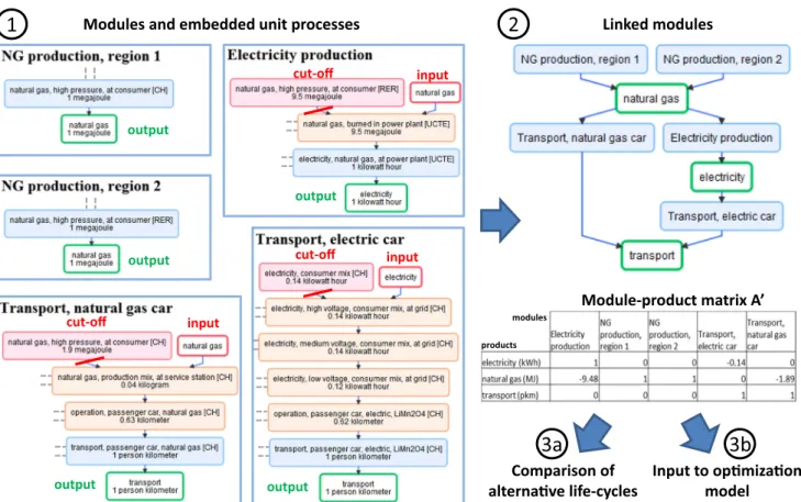
For example, the moduleBnatural gas production, region 1^producesnatural gasand is described in the LCI database by the processBnatural gas, high pressure, at consumer [CH],^ as shown in Fig.2 (step 1). The entire supply chain of this process is included, which means that the module relates to the life cycle ofBnatural gas, high pressure, at consumer [CH]^as modeled in ecoinvent. The downstream moduleBtransport, natural gas car^ producestransport and consumesnatural gasfor this. Based on their common input/output, these two modules can be linked to form a value chain fortransport. However, the moduleBtransport, natural gas car^links to the
ecoinvent inventory Btransport, passenger car, natural gas,^ which includes by default in its supply chain the production of natural gas. In order to avoid a double counting when com-bining the two modules into a value chain, a cutoff is intro-duced in the moduleBtransport, natural gas car.^
The linking of modules is based on product inputs and outputs. This can be described by a (possibly non-square) matrix, which we callmodule-product matrix(see Fig.2, step 2). It is different from the (square)technology matrixof LCI databases, which describes the linking of processes, in the sense that it truly distinguishes between modules (processes) and products and allows the same, substitutable, product to be the input or output of several modules. The drawback and reason why such matrices are not used in LCI databases is that they describe possible alternatives instead of predetermined value chains, which prohibits traditional ap-proaches to solve the inventory problem and perform LCA calculations (Heijungs and Suh2002; Suh and Huppes2005). Figure 2 (step 2) shows all the alternatives when connecting the modules. It includes two technology choices, with two alternatives each, resulting in a total of four different value chains for transport: the choice of natural gas from re-gion 1 or rere-gion 2, and the choice of a combustion engine car versus an electric vehicle. The corresponding module-product matrix is non-square, as it includes alternative suppliers for the substitutable products natural gas and transport.
In order to model and compare alternative value chains, the main work of the practitioner consists of defining suitable modules and their inputs and outputs (step 1), which depends on the study context. Steps (2) and (3a), the linking of modules and LCA calculations, can be performed by software for all alternative value chains (provided that each module produces one output only, see 0). In addition, the system of linked mod-ules can be directly integrated into an optimization model step
A1 A2
B2 B3
B1
C1 C2
D3 D4
D2
E2
E1 E3
D1
feedstock
feedstock, at consumer
feedstock, dried, stored
heat, at furnace
heat, at consumer
Feedstock producon
Transport
Storage & drying
Furnaces
Distribuon A) Compact representaon of
alternave life cycles (process-product linking)
B) Representaon in LCI databases (process-process linking)
life cycle modelled in LCI database alternave possibilies 2*3=6
2*3*2=12
2*3*2*4=48
2*3*2*4*3=144 2
Red numbers: alternave product life cycles Number of processes needed to model all alternaves in convenonal LCI databases: 2+6+12+48+144 = 212
A1 A2
B1-a2 B2-a1
B1-a1
C1-b1-a1 C1-b1-a2
B3-a1 B3-a2
B2-a2
C1-…
….
...
Legend
Fig. 1 aCompact representation of 144 alternatives to produce
(3b) (see 0). All steps in Fig.2, except for 3b, are supported in our open source modeling environment (Steubing2014).
2.2 The link between modules and the LCI database
If the supply chain of a module consists of unit processes from an LCI database, it can be specified by a final demand vectorf. The latter determines the scaling vectorsfor a given technol-ogy matrixA, as in Eq. (1). The scaling vector describes the necessary activity level for each process in the supply chain to meet the final demand and is the basis for further LCA calcu-lations (see Heijungs and Suh (2002) for a comprehensive introduction to matrix-based LCA).
s¼A−1f ð1Þ
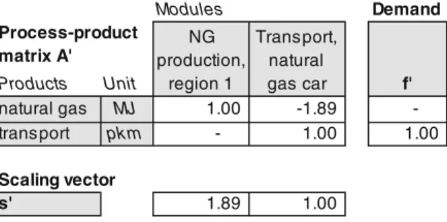
For example, the technology matrixAin Table1describes the inputs and outputs of the four processes shown in Fig.2for the moduleBtransport, natural gas car^ (data from ecoinvent v2.2, which includes 4087 interlinked processes; all other pro-cesses are excluded here for simplicity). The module refers to the supply chain forBtransport, passenger car, natural gas [CH],
^which is expressed by the demand vectorf1. As all processes are scaled to an output of one (diagonal values), the scaling vectors1informs us directly about the upstream inputs (see also Fig.2): For example, we need 1.89 MJ ofBnatural gas, high pressure, at consumer [CH]^to produce one person-kilometer of transport (0.63 × 0.064 × 46.9 = 1.89). However, with this demand vector, the module includes the production of natural gas. In order to define the desired upstream system boundary and avoid double counting, a cutoff needs to be implemented.
2.3 Cutoff implementation
To cutoff the production of natural gas and make the module represent a life cycle stage (as opposed to a full life cycle), the amount of natural gas that is required for one person-kilometer of transport is subtracted from the demand vector f2 as in Table1. As a result, the scaling factor of the processBnatural gas, high pressure, at consumer [CH]^becomes zero, which corresponds to a cutoff. In order to assure that the necessary input of natural gas is delivered by another module, it is stored in the module-product matrix (see Fig.2).
input
output
cut-off
cut-off input
output
output
cut-off input
output
s e l u d o m d e k n i L s
e s s e c o r p t i n u d e d d e b m e d n a s e l u d o M
output
Module-product matrix A’
Comparison of alternave life-cycles
1
2
3a
3b
Input to opmizaon model
modules
products
Fig. 2 Description of our modular LCA approach: (1) modules describe user-defined life cycle stages based on unit processes from an LCI data-base (ecoinvent). Cutoffs define upstream boundaries and avoid double counting. All other upstream inputs are by default included (gray dashed
2.4 LCA of a module
The environmental impacts related to a module can be calcu-lated as shown in Eq. (2), wherehis the environmental impact score of a module,Bis the biosphere matrix containing envi-ronmental interventions (e.g., emissions), andQis the charac-terization matrix that specifies the environmental impact per environmental intervention, see also Heijungs and Suh (2002).
h¼QBs ð2Þ
2.5 Comparing alternative value chains
The module-product matrix in Fig.2describes alternative val-ue chains whenever it contains several modules that produce substitutable products. While this is an efficient representation of alternatives, it does not allow regular LCA calculations directly, as suppliers cannot be uniquely identified (e.g., in Fig.2, it would be unclear whether natural gas would be delivered from region 1 or region 2). Therefore, an intermedi-ate step is required: For each alternative value chain contained in the module-product matrix, a smaller, square matrix needs to be constructed that uniquely links modules (as in conven-tional LCI databases). Based on this, LCA results can be cal-culated and compared for each alternative value chain.
2.5.1 Determining all alternatives
As shown in Fig.2, the module-product matrix has a graph representation that distinguishes two types of nodes: modules and products. A recursive depth-first graph traversal algorithm is used to determine all possible value chain combinations
contained in a module-product matrix. Its general logic is as follows: starting at the demanded product, the algorithm goes back through the value chains defined in the graph. When a product has multiple upstream producers, each of them will be considered in an alternative value chain. In contrast, when a module has several product inputs, all of them must be deliv-ered simultaneously. The algorithm and a figure describing this logic are provided in theElectronic Supplementary Material.
2.5.2 LCA calculations
For each alternative value chain, the module-product matrix is reduced to a smaller matrix that contains only those modules and products present in the alternative value chain. The result is a square module-product matrix where each module produces a unique product. The scaling vector for each module-product matrix can therefore be determined as in Eq. (3) (like in a regular LCI database). In the example of Fig. 2, if the value chain consists of the modules BNG production, region 1^ and Btransport, natural gas car,^the module-product matrixA′ rep-resents itself as in Table2. The moduleBNG production, region 1^produces one MJ ofnatural gasand does not have an input from the module-product matrix. The moduleBtransport, natural gas car^produces one person-kilometer oftransportand uses 1.89 U ofnatural gasfor this. This is reflected in the scaling vectors′for a demandf′of one person-kilometer transport.
s0 ¼Α0−1f0 ð3Þ
In order to do LCA calculations, we need to translate the demand f′ from the system of linked modules to a scaling vectorsof the technology matrix. The demand vectorsfthat
Table 1 Part of the supply chain of the moduleBTransport, natural gas car^(see Fig.2based on the technology matrix of ecoinvent 2.2. The demand vectorf1leads to the scaling vectors1. A cutoff for the input of
natural gas can be introduced by subtracting the demand of natural gas from the demand vectorf2, leading tos2
Processes Demand
Technology matrix A
t i n U s
t u p n I
MJ 1.00 -46.9 - - - -1.89
kg - 1.00 -0.064 - -
-km - - 1.00 -0.63 -
-pkm - - - 1.00 1.00 1.00
Scaling vectors
1.89
0.04 0.63 1.00
0.04 0.63 1.00 natural gas, high pressure, at
consumer [CH]
natural gas, production mix, at service station [CH]
operation, passenger car, natural gas [CH]
transport, passenger car, natural gas [CH]
s2
f1 f2
s1
natural gas, high pressure,
at consumer [CH]
natural gas, production mix, at service
station [CH]
operation, passenger car, natural gas [CH]
correspond to the individual modules can be summarized in a demand matrixF, which has one column for each module and as many rows as there are processes in the LCI database. Assuming that the order of columns and rows inF corre-sponds to the columns inA′andA, respectively, the translation of a product demand from the module-product matrix to a scaling vector for the LCI database can be realized as in Eq. (4).
s¼A−1FA0−1f0 ð4Þ
There is also a faster way to perform LCA calculations for many alternatives: It consists of first calculating the LCA re-sults for each module and then summing these up based on the scaling factors provided in s′. In this case, the number of
required LCA calculations scales with the number of modules instead of the number of alternative value chains.
2.6 Multifunctional modules
Some processes produce several products, such as refineries or combined heat and power plants. The integration of multi-functional processes in LCI databases may result in non-square, overdetermined technology matrices, for which tradi-tional methods fail to solve the inventory problem (Heijungs and Suh 2002). This problem is conventionally solved by system expansion or allocation (ISO2006a, b). Both ap-proaches lead to square technology matrices where each co-product can be demanded independently. While these ap-proaches could also be applied to multifunctional modules and the module-product matrix, it may, in some cases, be preferable to model multifunctional processes as they are in reality, i.e., considering their entire impacts, as well as the ratios of coproducts. For example, when designing chemical plants or energy systems, it is important to consider the inte-gration of coproducts to avoid suboptimal outcomes.
Multifunctional modules can be based on multioutput pro-cesses from unallocated versions of LCI databases. If such inventories are unavailable, multifunctional modules can be designed by combining allocated processes to resemble the original multifunctional process. Suppose that we have a tech-nology matrixA that contains two allocated processes that deliver heat and electricity from a joint production, as in Eq. (5). Let us further assume that for every unit of energy input, 50 % is converted to useful heat and 20 % to electricity. By specifying a demand vectorffor heat and electricity in the same ratio as in the original process, we can reproduce the inventory of the original process before allocation. At the same time, the products can be distinguished within the module-product matrix. Any demand of electricity from this module will then automatically result in a coproduction of heat and vice versa. Mathematically speaking, valid solutions for the scaling vectors′, expressed asA′s′= f′, are now limited
to linear combinations of the outputs of the module, e.g., 1 unit of heat and 0.4 units of electricity. Also,A′is now non-square and Eqs. (3) to (4) cannot be applied anymore. The use of multifunctional modules represents thus a trade-off: While additional information can be included to represent a system more realistically, other methods are required to identify fea-sible operating conditions for these systems. A method that is well suited to solve systems with such constraints is linear programming (Heijungs and Suh2002).
A¼ 1 0
0 1
; f ¼ 0:5
0:2
; A0 ¼ 0:5
0:2
ð5Þ
2.7 Using linked modules in optimization problems
LCA calculations for alternative value chains can be done efficiently as described above, as long as the described system does not include multioutput processes. If it does, or if other constraints shall be considered, a frequently used method to identify optimal solutions is to describe the system as an op-timization problem. While opop-timization problems can be very sophisticated, our intention here is to show how modules can be used as an input to an optimization problem in a straight-forward way. Several authors have shown that a basic formu-lation of an LCA-based optimization problem may look like the following (Azapagic and Clift1998; Heijungs and Suh 2002; Saner et al.2014; Tan et al.2008):
minimize h¼QBs ð6Þ
Subject to
As≥f ð7Þ
Equation (6), whereBandQare matrices for environmental interventions and their characterization, respectively, formu-lates the goal of the optimization—to minimize environmental impacts—and thereby provides a metric for choosing between alternatives. Eq. (7) determines the constraints of the system. It differs from matrix-based LCA by requiring the system’s out-put to be greater or equal than the final product demandf. This means that the solution may include product surpluses in cases where multioutput activities do not generate outputs in exactly the necessary ratios to satisfy the final demand. The decision variable in this context is the scaling vectors, which represents the use of technologies. An algorithm, such as the simplex algorithm, is usually applied to solve the optimization problem and identify the set of technologies that satisfy the product demand with minimal environmental impacts.
In the case of modules, it is theoretically possible to replaces
contain any decision variables. Instead, we suggest to pre-calculate the environmental impactshmfor each module using Eq. (2). The optimization problem can then be formulated as in Eqs. (8) and (9), where the total environmental impactshare the sum of the impacts of each modulehmmultiplied by the process-specific scaling factors′m, which is the decision variable.
minimize h¼X
m
s0mhm ð8Þ
Subject to
A0s0≥f0 ð9Þ
While this is the basic optimization model for modules, case-specific constraints may need to be added. An applica-tion of this model with addiapplica-tional constraints to a case study of the optimal use of wood is described in 3.2.
3 Application in case studies
3.1 Comparison of alternative scenarios for passenger car transport
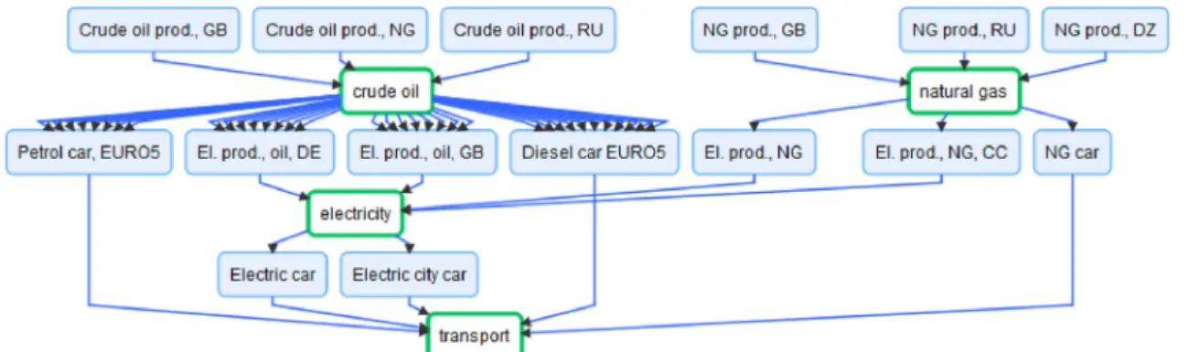
In order to illustrate some of the advantages of using modules, a strategic case study was developed around the topic of individ-ual mobility by extending the example in Fig.2. As shown in Fig.3, transportation, the functional unit of the system, can be provided by means of conventional combustion engines (die-sel, petrol, and natural gas) as well as by electric cars. Crude oil and natural gas have been considered as energy carriers, which can be converted either to transportation fuels or to electricity. Electricity can be generated with two different technologies for each energy carrier (for electricity from oil ecoinvent 2.2 dis-tinguishes country averages; for electricity from natural gas, an average and a state-of-the art natural gas combined cycle power plant are used). Additionally, we assume that the import source of the energy carriers can be influenced and for each imports from three different producing countries are included. Figure3 shows the product inputs and outputs for each module and the resulting system (details for each module are provided in the Electronic Supplementary Material).
The system contains 15 modules and 4 products. A total number of 33 alternative scenarios can be calculated automat-ically, as shown in Fig. 4. While no inventories have been specifically adapted for this illustration, this comparison based on ecoinvent 2.2 data shows that there are considerable differ-ences regarding the climate impact of these transportation sys-tems. As we distinguish products and modules, impact contri-butions along the value chain of each alternative can be expressed according to either one (Fig.4).
It can be observed that electric cars tend to perform better in this illustrative case study than cars with combustion engines. While the smaller electric city car performs better than the larger electric car, another important influence is the source of electricity, which can also lead to higher GHG emissions than combustion engines. In the case of combustion engines, diesel cars outperform petrol and natural gas cars. For the natural gas car, the source of natural gas plays an important role, due to differences in transportation distance and methane leakage.
Combustion engine-driven cars emit GHG emissions mainly at the transportation stage, while the main source of GHGs for electric cars is at the electricity generation stage. The observed GHG emissions at the transportation stage for electric cars arise from the fact that this stage also includes the road infrastructure and maintenance. While this could easily have been excluded or modeled as aBroad^input, we leave it here at this to remind the reader that the definition of what a module comprises and how its products are called is case-specific and up to the practitioner.
3.2 Optimal use of wood in a cascading system
3.2.1 Model description
In order to illustrate how modules (including multioutput ones) can be used within an optimization problem, we devised a linear programming case study around the use of forest wood for material and energy applications. The central ques-tion raised is whether it is environmentally beneficial to use wood in cascades, i.e., first for a material applications and then for energy. As the case study is of illustrative nature, we limit the discussion to GHG emissions, although other impact cat-egories could be assessed with the same model.
Table 2 Module-products matrix for the transport by natural gas car
Modules Demand
Products Unit
natural gas MJ 1.00 -1.89 -transport pkm - 1.00 1.00
Scaling vector
s' 1.89 1.00
Process-product matrix A'
NG production,
region 1
Transport, natural
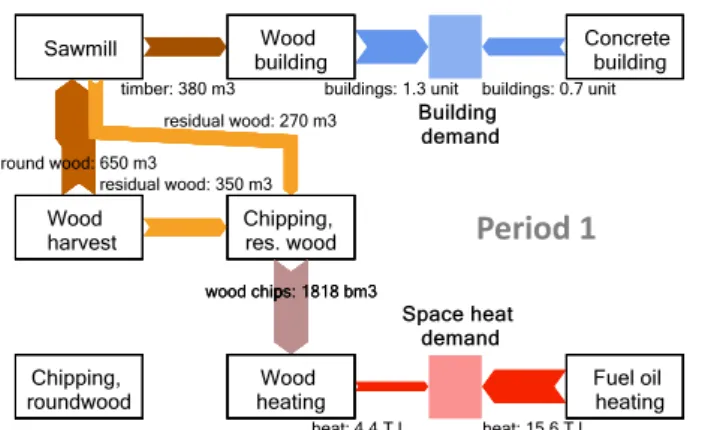
In an attempt to capture the most important processes, the wood value chain was simplified to include the following mod-ules (Fig.5): The processBwood harvest^describes everything from tree planting, forest maintenance and harvest to the pro-duction ofround wood. Round wood can be further processed in aBsawmill^ totimber. Timber can be used to construct Bwood buildings.^The modulesBwood harvest,^Bsawmill,^ andBwood building^are modeled as multioutput modules as each of them also producesresidual wood(forest and sawmill residues as well as residual wood from the wood building at its end-of-life). The processBchipping, residual wood^ can pro-ducewood chipsfrom residual wood, which can be used in a Bwood chips heating^ to produce heat. Alternatively, wood chips can be produced directly from round wood, i.e., without a previous material use, by the process Bchipping, round wood.^ Inventories for the modules are based on ecoinvent 2.2, except for the wood and concrete buildings, which are based on Gustavsson et al. (2006) (details are provided in the Electronic Supplementary Material).
We assume that the demand from this system is 2 buildings and 20 TJ heat, which represent, respectively, material and energy applications of wood. A supply constraint applies for the harvest of forest wood, which is assumed to be limited to 1000 m3(as round wood and residual wood are coproduced at a ratio of 0.65 to 0.35, respectively, their supplies are limited to 650 and 350 m3). Due to this constraint, wood alone is insufficient to meet the product demand. To provide conven-tional alternatives, the processesBconcrete building^andBfuel oil heating^are included.
We also extend the optimization model with time periods and two types of stocks: one for harvestable wood in the forest and one for timber in buildings. The harvestable wood stock increases each period by 1000 m3, and we assume that wood left in the forest can be harvested in later periods without losses. Timber in buildings on the other hand has a discrete lifespan: once the building is demolished, it becomes residual wood. For the sake of simplicity, our model includes two time periods of the length of a building lifespan (e.g., 60 years).
Fig. 3 Use of modules to construct a system that describes alternative value chains for transportation (several arrowsindicate that several suppliers were cutoff in a module)
product contribuon
module contribuon
After each period, all of the previously stored timber becomes residual wood and is burned to produce energy.
The model objective is to minimize the environmental im-pactsh, which are the sum of the impacts of the individual modules times their use over all time periods (10) (see Table3 for nomenclature). The constraints are the following: The de-mand (D) needs to be satisfied by the product flows during each time period (11). The product flows (PF) are the result of the scaling of the modules in the system and the flows to and from stocks (ST) (12). Note that due to the introduction of stocks, the product flows may temporally differ from the flows as prescribed by the modules. Product lifetimes (L) are spec-ified for each module in a matrix. The values of L are used in Eq. (13) to add or remove products from the stock, depending on the current and previous use of processes where storage occurs. In this case study, only wood in buildings is added to the stock and removed one period later. Finally, the harvest-able wood stock (hws) is modeled as the difference of previ-ously available and newly added harvestable wood (hw, 1000 m3per period) and its use in the processBwood harvest^ as described by Eq. (14). Neither the scaling factors of mod-ules nor the amount of products stored can become negative in reality, which is expressed by Eq. (15). The model was solved using the GAMS software (GAMS2013).
min h¼X
m;t
S0m;thm ð10Þ
Subject to
Dp;t≤
X
m
P Fp;m;t ∀p;t ð11Þ
P Fp;m;t¼A
0
p;mS
0
m;tþSTp;m;t−1−STp;m;t ∀p;m;t ð12Þ
STp;m;t¼STp;m;t−1þA
0
p;m S
0
m;t−S
0
m;t−Lm;p
∀p;m;t ð13Þ
hwst¼hwst−1þhwt−
X
p
X
m A0p;mS
0
m;t
∀t;p∈pwood;m∈mharvest
ð14Þ
S0m;t;STp;m;thwst≥0 ∀p;m;t ð15Þ
3.2.2 Results
As shown in Fig.5, the building and heating demand can only partly be satisfied by wood. The remainder is delivered by means of conventional technologies. The model was set up like this to reflect the fact that wood is a scarce resource in many countries. As wood cannot fully supply the product demand, the optimization model uses it for those applications with the highest environmental leverage. As a result, round wood is used entirely for material applications in period 1, whereas it is used entirely for direct energy purposes in period 2. The reason for this behavior is that the substitution of fuel oil for heating yields a higher benefit per unit wood used than the use of wood in buildings. The reason why round wood is used in a material way despite lower direct benefits is the fact that the end-of-life residual wood from buildings can be reused energetically in period 2. Since there are only two periods, round wood in period 2 is directly used for energy.
4 Discussion
4.1 Modular LCA approach
4.1.1 Areas of application
Modules, as described in this paper, can serve different pur-poses in different types of LCA studies (Fig.6). An immediate benefit is a simplified representation of product value chains according to the system boundaries of the modules, which may reflect those aspects that are relevant to a specific actor. This may help practitioners to effectively analyze the implica-tions of key choices and communicate LCA results. In con-trast to system processes, where the whole supply chain is aggregated into a single inventory, modules do not prohibit contribution analyses from underlying unit processes.
buildings: 2 unit
buildings: 1.3 unit buildings: 0.7 unit
timber: 380 m3
residual wood: 270 m3
round wood: 650 m3
residual wood: 350 m3 residual wood: 350 m3
Period 1
Period 2
round wood: 650 m3 wood chips: 2141 bm3
wood chips: 1818 bm3 wood chips: 1818 bm3 p p
heat: 10 3 TJ heat: 9 7 TJ
wood chips: 1906 bm3 heat: 15.6 TJ
heat: 4.4 TJ
residual wood: 380 m3
In the context of explorative studies, the modular LCA approach offers a powerful tool to model and compare alter-native value chains, possibly reducing the necessary time in-vestment (see also 4.1.1.). A key element is the module-product matrix that links modules based on module-product inputs and outputs. It is a compact representation of alternative value chains, without the need for additional copies of datasets for alternative suppliers as in conventional LCI databases. How-ever, it relies on the assumption that products from alternative suppliers are in fact substitutable. It is the responsibility of the practitioner to check whether this can be justified in a given context. As modules are most likely tailored to a specific con-text, a drawback is that they may not be reusable in a different context.
Modules can also be used in optimization models. This provides the possibility to add aspects that are not included in a standard LCA, such as multifunctional modules or con-straints. Further, the temporal dimension (Beloin-Saint-Pierre et al.2014; Finnveden et al.2009; Levasseur et al.2010) and
the change of material stocks are important parameters that are generally not considered in LCA studies (Cherubini et al. 2011; Levasseur et al.2012; Pauliuk and Müller2014). The case study illustrates that six equations are sufficient to formu-late an optimization problem that extends the LCA model with a simple temporal dimension, stocks, and supply and demand constraints. The use of modules could therefore potentially facilitate the combination of LCA with other industrial ecolo-gy methods such as material flow analysis (MFA). Modules could also be used in combination with input-output analysis (IOA) to describe the environmental impacts related to eco-nomic sectors with consistent system boundaries (i.e., cutoffs).
4.1.2 Unlocking the hidden potential of LCI databases
While LCI databases contain many specific inventories, they are designed to describe average value chains as opposed to all possible alternatives. For example, ecoinvent version 3
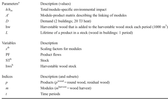
Table 3 Parameters, variables, and indices used in the optimization model
Parametersa Description (values)
h/hm Total/module-specific environmental impact
A′ Module-product matrix describing the linking of modules
D Demand (2 buildings; 20 TJ heat)
hw Harvestable wood that is added to the harvestable wood stock each period (1000 m3)
L Lifetime of a product in a stock (wood in buildings: 1 period)
Variables Description
s′b Scaling factors for modules
PF Product flows
STb Stock
hwsb Harvestable wood stock
Indices Description (and subsets)
p Products (pwood= round wood, residual wood)
m Modules (mharvest= wood harvest)
t Time periods
a
Same values for each time period b
Variable must be positive, see Eq. (15)
Many alternaves, explorave LCA, mul-output processes, constraints. LCA based opmizaon problem. Many alternaves, explorave LCA. Broad comparison and idenficaon
of best soluons.
Few or no alternaves. Product focus. Classical product LCA or comparison.
input to opmizaon problem (case study 2) (connecon to MFA, IO, etc.)
automac, efficient comparison of alternaves
(case study 1) life cycle stage based representaon and impact
assessment
Type of LCA study
Usefulness of modules
complexity
(Ecoinvent2015) contains different inventories for the gener-ation of electricity, depending on the energy source, but then combines all producers of electricity in a geographical region into a market to represent a production volume weighted av-erage electricity mix (Treyer and Bauer2014; Weidema et al. 2013). Downstream consumers are by default linked to the market mix, while direct links to specific electricity producers are the exception. Therefore, many alternative value chains— for which inventories exist—are not readily available to the practitioner. The transportation case study is a good example showing how modules can help to unlock the additional po-tential of inventories that are contained in LCI databases. Nat-urally, it is the responsibility of the practitioner to combine inventories in a meaningful way. Version 3 of ecoinvent has made an interesting development supporting this by formally distinguishing between processes and products. As a result, the same product (e.g.,Belectricity, high voltage^) may now be produced by several activities. This facilitates the search for alternative producers of substitutable products and, therefore, the design of modules.
4.1.3 Do practitioners gain time?
LCA studies are usually done under time constraints. Using modules to perform, e.g., scenario analyses, is associated with an up-front time investment. From our experience, much of it is related to developing a better system understanding, which enables the definition of suitable system boundaries to capture the key choices in modules. At the same time, modeling alter-natives in conventional LCA software may be equally time-consuming or even limiting, e.g., if 212 processes need to be modeled like in the example of Fig.1. A further consideration is that error corrections or sensitivity analyses can be realized much quicker in a small number of modules than with many processes. A clear advantage of the modular approach is also that the LCA calculation time scales with the number of mod-ules and not with the number of alternatives (i.e., using the example of the introduction, 14 calculations instead of 144). As LCA is usually an iterative procedure, this can be relevant. Nevertheless, whether practitioners save time by applying the modular approach depends on the complexity of the system, the practitioner’s knowledge and modeling skills, and the LCA software itself.
4.1.4 Software implementation
In order to perform the individual modeling steps, we have developed the Activity Browser (Steubing2014), which is an open source LCA software with a graphical user interface that builds upon the brightway2 LCA framework (Mutel2015). The source code and documentation are provided online for the LCA community to apply and further develop the present-ed approach or to include it in other LCA software.
4.2 Case studies
Two case studies illustrate the application of the module framework for modeling and comparing alternatives as well as for extending an LCA problem to include constraints, a temporal dimension, and stocks. While they are mainly of illustrative nature, they are based on inventories from the ecoinvent database, which are regularly used as a reference within the LCA community and beyond. The comparison of 33 passenger car transportation alternatives showed that elec-tric cars could significantly reduce GHG emissions compared to cars using conventional fuels. However, the size of the car, the battery, and the electricity source have substantial influ-ence on environmental performance and may also make elec-tric cars perform worse than conventional ones.
Regarding the optimal use of wood, we show that using wood in a use cascade, i.e., first for material and then for energy applications, may be advantageous for mitigating cli-mate change. However, the potentially significant time gap between the material and the energy use (as much as a build-ing’s life time) adds ambiguity to this conclusion as it is diffi-cult to predict what will be the alternative (substitution) to wood energy in the future (Gärtner et al.2013). Further, the assumption that wood substitutes other material or energy sources needs to be carefully examined (Gustavsson and Sathre 2011). These and other factors, such as the relation between product design, recycling efficiencies, and end-of-life energy substitution (Höglmeier et al.2015), should be further investigated to better understand the conditions for an environmentally beneficial cascading of wood.
5 Conclusions
scenario analyses, as illustrated by the transportation case study.
The modular approach can also serve other purposes, such as yielding a simplified the representation of a life cycle for communication purposes. The use of modules to formulate an optimization model enables the consideration of constraints and acts as a potential bridge to other industrial ecology methods, such as MFA and IOA.
The creation of modules and an automated scenario analy-sis are supported within an open source LCA software. How-ever, the approach is generic and could be implemented in other software as well.
Acknowledgments This research was funded within the National Re-search ProgrammeBResource Wood^(NRP 66,www.nfp66.ch) by the Swiss National Science Foundation (project no. 136612). We would like to thank the two anonymous reviewers as well as Carl Vadenbo for their valuable input.
Open AccessThis article is distributed under the terms of the Creative C o m m o n s A t t r i b u t i o n 4 . 0 I n t e r n a t i o n a l L i c e n s e ( h t t p : / / creativecommons.org/licenses/by/4.0/), which permits unrestricted use, distribution, and reproduction in any medium, provided you give appropriate credit to the original author(s) and the source, provide a link to the Creative Commons license, and indicate if changes were made.
References
Azapagic A, Clift R (1998) Linear programming as a tool in life cycle assessment. Int J Life Cycle Assess 3:305–316
Azapagic A, Clift R (1999) Life cycle assessment and multiobjective optimisation. J Clean Prod 7:135–143
Beloin-Saint-Pierre D, Heijungs R, Blanc I (2014) The ESPA (Enhanced Structural Path Analysis) method: a solution to an implementation challenge for dynamic life cycle assessment studies. Int J Liffe Cycle Assess 19:861–871
Buxmann K, Kistler P, Rebitzer G (2009) Independent information modules-a powerful approach for life cycle management. Int J Life Cycle Assess 14:S92–S100
Cherubini F, Peters GP, Berntsen T, Strømman AH, Hertwich E (2011) CO 2 emissions from biomass combustion for bioenergy: atmo-spheric decay and contribution to global warming. GCB Bioenergy 3:413–426
Ecoinvent (2015) The ecoinvent LCA database,http://www.ecoinvent.ch/ Finnveden G, Hauschild MZ, Ekvall T, Guinée JB, Heijungs R, Hellweg S, Koehler A, Pennington D, Suh S (2009) Recent developments in Life Cycle Assessment. J Environ Manage 91:1–21
GAMS (2013) GAMS Development Corporation. General Algebraic Modeling System (GAMS) Release 24.2.1., Washington, DC, USA,http://www.gams.com/
Gärtner S, Hienz G, Keller H, Müller-Lindenlauf M (2013) Gesamtökologische Bewertung der Kaskadennutzung von Holz– U m w e l t a u s w i r k u n g e n s t o f f l i c h e r u n d e n e r g e t i s c h e r Holznutzungssysteme im Vergleich. Institut für Energie- und Umweltforschung (IFEU), Heidelberg, Germany
Gassner M, Maréchal F (2009) Methodology for the optimal thermo-economic, multi-objective design of thermochemical fuel produc-tion from biomass. Comput Chem Eng 33:769–781
Guillén-Gosálbez G (2011) A novel MILP-based objective reduction method for multi-objective optimization: application to environmen-tal problems. Comput Chem Eng 1469–1477
Guillén-Gosálbez G, Grossmann I (2010) A global optimization strategy for the environmentally conscious design of chemical supply chains under uncertainty in the damage assessment model. Comput Chem Eng 42–58
Guillén-Gosálbez G, Caballero JA, Esteller LJ, Gadalla M (2007) Application of life cycle assessment to the structural optimization of process flowsheets. In: Serban AP (ed) Valentin P. Elsevier, Computer Aided Chemical Engineering, pp 1163–1168
Gustavsson L, Sathre R (2011) Energy and CO2 analysis of wood sub-stitution in construction. Climatic Change 129–153
Gustavsson L, Pingoud K, Sathre R (2006) Carbon dioxide balance of wood substitution: comparing concrete- and wood-framed build-ings. Mitig Adapt Strateg Glob Chang. 667–691
Heijungs R, Suh S (2002) The computational structure of life cycle as-sessment. Kluwer, Dordrecht, The Netherlands
Höglmeier K, Steubing B, Weber-Blaschke G, Richter K (2015) LCA-based optimization of wood utilization under special consideration of a cascading use of wood. J Environ Manage:158–170. ISO (2006a) ISO 14040. Environmental management - Life cycle
assess-ment - Principles and framework. International Standardization Organization, Geneva, Switzerland, pp 28
ISO (2006b) ISO 14025. Environmental labels and declarations - type III environmental declarations - Principles and procedures. ISO/TC 207/SC3. International Organization for Standardization, Brussels ISO 14048 (2002) Environmental management—Life cycle assessment
—Data documentation format. International Organization for Standardization (ISO), Geneva
Jungbluth N, Tietje O, Scholz RW (2000) Food purchases: impacts from the consumers’point of view investigated with a modular LCA. Int J LCA 134–142
Levasseur A, Lesage P, Margni M, Deschěnes L, Samson R (2010) Considering time in LCA: dynamic LCA and its ap-plication to global warming impact assessments. Environ Sci Technol 3169–3174
Levasseur A, Lesage P, Margni M, Brandão M, Samson R (2012) Assessing temporary carbon sequestration and storage projects through land use, land-use change and forestry: comparison of dy-namic life cycle assessment with ton-year approaches. Climatic Change 759–776
Mutel C (2015) A new open source framework for advanced life cycle assessment calculations.,http://brightwaylca.org/
Pauliuk S, Müller DB (2014) The role of in-use stocks in the social metabolism and in climate change mitigation. Glob Environ Chang 132–142. doi:10.1016/j.gloenvcha.2013.11.006
Rebitzer G (2005) Enhancing the application efficiency of life cycle as-sessment for industrial uses. Int J LCA: 446. doi:10.1065/lca2005. 11.005
Saner D, Vadenbo C, Steubing B, Hellweg S (2014) Regionalized LCA-based optimization of building energy supply: method and case study for a swiss municipality. Environ Sci Technol 7651–7659 Steubing B (2014) Activity Browser - A free and extendable LCA
soft-ware.,https://bitbucket.org/bsteubing/activity-browser
Suh S, Huppes G (2005) Methods for life cycle inventory of a product. J Clean Prod 687–697
Tan RR (2008) Using fuzzy numbers to propagate uncertainty in matrix-based LCI. Int J LCA 585–592
Tan RR, Culaba AB, Aviso KB (2008) A fuzzy linear programming extension of the general matrix-based life cycle model. J Clean Prod. 1358–1367
Vadenbo C, Hellweg S, Guillén-Gosálbez G (2014) Multi-objective optimization of waste and resource management in industrial networks - Part I: model description. Resour Conserv Recy 52–63
Weidema B, Bauer C, Hischier R, Mutel CL, Nemecek T, Reinhard J, Vadenbo CO, Wernet G (2013) Overview and methodology. Data
quality guideline for the ecoinvent database version 3. ecoinvent Centre