Sterile Neutrino Dark Matter
A. Boyarskya, M. Drewesb,c, T. Lasserred,e,f,g, S. Mertensf,h, O. Ruchayskiyi
aUniversiteit Leiden - Instituut Lorentz for Theoretical Physics, P.O. Box 9506, NL-2300 RA Leiden, Netherlands
bCentre for Cosmology, Particle Physics and Phenomenology, Universit´e catholique de Louvain, Louvain-la-Neuve B-1348, Belgium
cExcellence Cluster Universe, Boltzmannstr. 2, D-85748, Garching, Germany
dCommissariat `a l’´energie atomique et aux ´energies alternatives, Centre de Saclay,DRF/IRFU, 91191 Gif-sur-Yvette, France
eInstitute for Advance Study, Technische Universit¨at M¨unchen, James-Franck-Str. 1, 85748 Garching fPhysik-Department, Technische Universit¨at M¨unchen, James-Franck-Str. 1, 85748 Garching gAstroParticule et Cosmologie, Universit´e Paris Diderot, CNRS/IN2P3, CEA/IRFU, Observatoire de
Paris, Sorbonne Paris Cit´e, 75205 Paris Cedex 13, France
hMax-Planck-Institut f¨ur Physik (Werner-Heisenberg-Institut), Foehringer Ring 6, 80805 M¨unchen, Germany
iDiscovery Center, Niels Bohr Institute, Copenhagen University, Blegdamsvej 17, DK-2100 Copenhagen, Denmark
Abstract
We review sterile neutrinos as possible Dark Matter candidates. After a short summary on the role of neutrinos in cosmology and particle physics, we give a comprehensive overview of the current status of the research on sterile neutrino Dark Matter. First we discuss the motivation and limits obtained through astrophysical observations. Second, we review different mechanisms of how sterile neutrino Dark Matter could have been produced in the early universe. Finally, we outline a selection of future laboratory searches for keV-scale sterile neutrinos, highlighting their experimental challenges and discovery potential.
Keywords: neutrino: sterile — neutrino: dark matter — neutrino: production — neutrino: model — cosmological model — neutrino: oscillation — neutrino: detector — new physics — review
Contents
1 Dark Matter in the Universe 3
1.1 Standard Model Neutrino as Dark Matter Candidate? . . . 3
1.2 Solution to Dark Matter Puzzle in Different Approaches to BSM Physics . . . 4
1.3 Heavy ”Sterile” Neutrinos . . . 5
2 Neutrinos in the Standard Model and Beyond 6 2.1 Neutrinos in the Standard Model . . . 7
2.2 The Origin of Neutrino Mass . . . 9
2.3 Neutrino mass and New Physics . . . 10
2.4 Sterile Neutrinos . . . 14
2.4.1 Right Handed Neutrinos and Type-I Seesaw . . . 14
2.4.2 Low Scale Seesaw . . . 16
2.4.3 The Neutrino Minimal Standard Model . . . 18
3 Properties of Sterile Neutrino Dark Matter 18 3.1 Phase Space Considerations . . . 19
3.2 Decaying Dark Matter . . . 19
3.2.1 Existing Constraints . . . 19
3.2.2 Status of the 3.5 keV Line . . . 22
3.3 Sterile Neutrinos and Structure Formation . . . 24
3.3.1 Warm Dark Matter . . . 24
3.3.2 Lyman-αForest Method . . . 26
3.3.3 Measuring Matter Power Spectrum via Weak Gravitational Lensing . . . 28
3.3.4 Counting halos . . . 28
3.4 Other Observables . . . 29
4 keV-Scale Sterile Neutrino Dark Matter Production in the Early Universe 31 4.1 Overview . . . 31
4.2 Thermal Production via Mixing (“freeze in”) . . . 32
4.2.1 Non-resonant Production . . . 32
4.2.2 Resonant Production . . . 34
4.2.3 Treatment in Quantum Field Theory . . . 36
4.2.4 Uncertainties and Open Questions . . . 39
4.3 Thermal Production via New Gauge Interactions (“freeze out”) . . . 40
4.4 Non-thermal Production in the Decay of Heavier Particles . . . 42
5 Laboratory Searches for keV-scale Sterile Neutrinos 45 5.1 Overview . . . 45
5.2 Direct Detection . . . 45
5.2.1 Sterile Neutrino Capture . . . 46
5.2.2 Sterile Neutrino Scattering . . . 51
5.3 Detection through Sterile Neutrino Production . . . 51
5.3.1 Beta Decay Spectroscopy . . . 51
5.3.2 Full Kinematic Reconstruction . . . 56
1. Dark Matter in the Universe
There is a body of strong and convincing evidence that most of the mass in the observable universe is not composed of known particles. Indeed, numerous independent tracers of the gravitational potential (observations of the motion of stars in galaxies and galaxies in clusters; emissions from hot ionised gas in galaxy groups and clusters; 21 cm line in galaxies; both weak and strong gravitational lensing measurements) demonstrate that the dynamics of galaxies and galaxy clusters cannot be explained by the Newtonian potential created by visible matter only. Moreover, cosmological data (analysis of the cosmic microwave background anisotropies and of the statistics of galaxy number counts) show that the cosmic large scale structure started to develop long before decoupling of photons due to the recombination of hydrogen in the early Universe and, therefore, long before ordinary matter could start clustering. This evidence points at the existence of a new substance, universally distributed in objects of all scales and providing a contribution to the total energy density of the Universe at the level of about 27%. This hypothetical new substance is commonly known as ”Dark Matter” (DM). The DM abundance is often expressed in terms of the density parameter ΩDM = ρDM/ρ0,
where ρDM is the comoving DM density and ρ0 = 3H2m2P l/(8π) is the critical density of the universe, with H the Hubble parameter and mP l the Planck mass. Current measurements suggest ΩDMh2 = 0.1186 ±0.0020, where h is H in units 100 km/(s Mpc) [1]. Different
aspects of the DM problem can be found in reviews [2–4], for historical exposition of the problem see [3, 5, 6]. Various attempts to explain this phenomenon by the presence of macroscopic compact objects (such as, for example, old stars [7–10]) or by modifications of the laws of gravity (for a review see [11–13]) failed to provide a consistent description of all the above phenomena (see the overviews in [13, 14]). Therefore, a microscopic origin of DM phenomenon, i.e., a new particle or particles, remains the most plausible hypothesis.1
1.1. Standard Model Neutrino as Dark Matter Candidate?
The only electrically neutral and long-lived particles in the Standard Model (SM) of particle physics are the neutrinos, the properties of which are briefly reviewed in Sec. 2
(cf. e.g. [16] for a review of neutrinos in cosmology). As experiments show that neutrinos have mass, they could in principle play the role of DM particles. Neutrinos are involved in weak interactions (3) that keep them in thermal equilibrium in the early Universe down to the temperatures of few MeV. At smaller temperatures, the interaction rate of weak reactions drops below the expansion rate of the Universe and neutrinos “freeze out” from the equilibrium. Therefore, a background of relic neutrinos was created just before primordial nucleosynthesis. As interaction strength and, therefore, decoupling temperature of these particles are known, one can easily find that their number density, equal per each flavour to
nα = 6 4
ζ(3) π2 T
3
ν (1)
1Primordial black holes that formed prior to the baryonic acoustic oscillations visible in the sky are one
where Tν '(4/11)1/3Tγ '1.96K'10−4 eV.2 The associated matter density of neutrinos at late stage (when neutrinos are non-relativistic) is determined by the sum of neutrino masses
ρν 'nα X
mi (2)
To constitute the whole DM this sum should be about 11.5 eV (see e.g. [16]). Clearly, this is in conflict with the existing experimental bounds: measurements of the electron spectrum of β-decay put the combination of neutrino masses below 2 eV [17] while from the cosmological data one can infer an upper bound of the sum of neutrino masses varies between 0.58 eV at 95% CL [18] and 0.12 eV [19, 20], depending on the dataset included and assumptions made in the fitting. The fact that neutrinos could not constitute 100% of DM follows also from the study of phase space density of DM dominated objects that should not exceed the density of degenerate Fermi gas: fermionic particles could play the role of DM in dwarf galaxies only if their mass is above few hundreds of eV (the so-called ’Tremaine-Gunn bound’ [21], for review see [22] and references therein) and in galaxies if their mass is tens of eV. Moreover, as the mass of neutrinos is much smaller than their decoupling temperature, they decouple relativistic and become non-relativistic only deeply in matter-dominated epoch (“Hot Dark Matter”). For such a DM candidate the history of structure formation would be very different and the Universe would look rather differently nowadays [23]. All these strong arguments prove convincingly that the dominant fraction of DM can not be made of the known neutrinos and thereforethe Standard Model of elementary particles does not contain a viable DM candidate.
1.2. Solution to Dark Matter Puzzle in Different Approaches to BSM Physics
The hypothesis that DM is made of particles necessarily implies an extension of the SM with new particles. This makes the DM problem part of a small number of observed phenom-ena in particle physics, astrophysics and cosmology that clearly point towards the existence of “New Physics”. These major unsolved challenges are commonly known as “beyond the Standard Model” (BSM) problems and include
I) Dark Matter: What is it composed of, and how was it produced?
II) Neutrino oscillations: Which mechanism gives masses to the known neutrinos?
III) Baryon asymmetry of the Universe: What mechanism created the tiny matter-antimatter asymmetry in the early Universe? This baryon asymmetry of the universe (BAU) is believed to be the origin of all baryonic matter in the present day universe after mutual annihilation of all other particles and antiparticles, cf. e.g. [24].
IV) The hot big bang: Which mechanism set the homogeneous and isotropic initial conditions of the radiation dominated epoch in cosmic history? In particular, if the initial state was created during a stage of accelerated expansion (cosmic inflation), what was driving it?
In addition to these observational puzzles, there are also deep theoretical questions about the structure of the SM: the gauge hierarchy problem, strong CP-problem, the cosmological constant problem, the flavour puzzle and the question why the SM gauge group is SU(3)×
SU(2)×U(1). Some yet unknown particles or interactions would be needed to answer these questions.
Perhaps, most of the research in BSM physics during the last decades was devoted to a solution of thegauge hierarchy problem, i.e. the problem of quantum stability of the mass of the Higgs boson against radiative corrections. The requirement of the absence of quadrati-cally divergent corrections to the Higgs boson is an example of so-called “naturalness”, cf. eg. [25]. Quite a number of different suggestions were proposed on how the “naturalness” of the electroweak symmetry breaking can be achieved. They are based on supersymmetry, technicolour, large extra dimensions or other ideas. Most of these approaches postulate the existence of new particles that participate in electroweak interactions. Therefore in these models weakly interacting massive particles (WIMPs) appear as natural DM candidates. WIMPs generalise the idea of neutrino DM [26]: they also interact with the SM sector with roughly electroweak strength, however their mass is large (from few GeV to hundreds of TeV), so that these particles are already non-relativistic when they decouple from primor-dial plasma. This suppresses their number density and they easily satisfy the lower mass bound that ruled out the known neutrinos as DM. In this case the present day density of such particles depends very weakly (logarithmically) on the mass of the particle as long as it is heavy enough. This “universal” density happens to be within the order of magnitude consistent with DM density (the so-called “WIMP miracle”). WIMPs are usually stable or very long lived, but can annihilate with each other in the regions of large DM densities, producing a flux of γ-rays, antimatter and neutrinos. However, to date, neither particle colliders nor any of the large number of direct and indirect DM searches could provide con-vincing evidence for the existence of WIMPs. This provides clear motivation to investigate alternatives to the WIMP paradigm. Indeed, there exist many DM candidates that differ by their mass, interaction types and interaction strengths by many order of magnitude (for reviews see e.g. [27–29]).
1.3. Heavy ”Sterile” Neutrinos
bounds on their parameters. There exist a larger number of models that accommodate this possibility, see e.g. [43] for a review.
The present article provides an update of the phenomenological constraints on sterile neutrino DM. In Sec. 2 we briefly review the role of neutrinos in particle physics and define our notation. We in particular address the idea of heavy sterile neutrinos in Sec. 2.4. In Sec.3we provide an overview of the observational constraints on sterile neutrino DM. These partly depend on the way how the heavy neutrinos were produced in the early universe. Different production mechanisms are reviewed in Sec. 4. Sec. 5 is devoted to laboratory searches for DM sterile neutrinos. We finally conclude in Sec. 6.
2. Neutrinos in the Standard Model and Beyond
Neutrinos are the most elusive known particles. Their weak interactions make it very difficult to study their properties. At the same time, there are good reasons to believe that neutrinos may hold a key to resolve several mysteries in particle physics and cosmology. Neutrinos are unique in several different ways.
• Neutrinos are the only fermions that appear only with left handed (LH) chirality in the SM.
• In the minimal SM, neutrinos are massless. The observed neutrino flavour oscillations clearly indicate that at least two neutrinos have non-vanishing mass. In the framework of renormalisable quantum field theory, the existence of neutrino masses definitely implies that some new states exist, see Sec.2.3. This is why neutrino masses are often referred to as the only sign of New Physics that has been found in the laboratory.3
• The neutrino masses are much smaller than all other fermion masses in the SM. The reason for this separation of scales is unclear. This is often referred to as the mass puzzle.
• The reason why neutrinos oscillate is that the quantum states in which they are pro-duced by the weak interaction (interaction eigenstates) are not quantum states with a well defined energy (mass eigenstates). The misalignment between both sets of states can be described by a flavour mixing matrix Vν in analogy to the mixing of quarks by the Cabibbo-Kobayashi-Maskawa (CKM) matrix.4 However, while the CKM matrix is
very close to unity, the neutrino mixing matrix Vν looks very different and shows no clear pattern. This is known as the flavour puzzle.
3This ”New Physics” could in principle be fairly boring if it only consists of new neutrino spin orientations,
cf. the discussion following Eq. (8), or could provide a key to understand how the SM is embedded in a more fundamental theory of nature, cf. sec.2.3.
4In the basis where charged Yukawa couplings are diagonal, the mixing matrix V
ν is identical to the
We refer to the three known neutrinos that appear in the SM as active neutrinos because they feel the weak interaction with full strength. This is in contrast to the hypothetical sterile neutrinos that e.g. may compose the DM, which are gauge singlets. In the following we very briefly review some basic properties of neutrinos before moving on to the specific topic of sterile neutrinos as DM candidates; for a more detailed treatment we e.g. refer the reader to ref. [46].
2.1. Neutrinos in the Standard Model
Neutrinos can be produced in the laboratory in two different ways. On one hand, they appear as a by-product in nuclear reactions, and commercial nuclear power plants generate huge amounts of neutrinos ”for free”. The downside is that the neutrinos are not directed, and their energy spectrum is not known with great accuracy. On the other hand, a neutrino can be produced by sending a proton beam on a fixed target. The pions that are produced in these collisions decay into muons and neutrinos. Both mechanisms are, in a similar way, also realised in nature. Neutrinos from nuclear reactions in nature include the solar neutrinos are produced in fusion reactions in the core of the sun and a small neutrino flux due to the natural radioactivity in the soil. Atmospheric neutrinos, on the other hand, are produced in the cascade of decays following high energy collisions of cosmic rays with nuclei in the atmosphere. A large number of experiments has been performed to study neutrinos from all these sources. In the following we briefly summarise the combined knowledge that has been obtained from these efforts, without going into too experimental details.
In the SM, there exist three neutrinos. They are usually classified in terms of their interaction eigenstates να, where α = e, µ, τ refers to the “family” or “generation” each of them belongs to,5 and referred to as “electron neutrino”, “muon neutrino” and “tau neutrino”. This convention is in contrast to the quark sector, where the particle names u,d, s, c, b and t refer to mass eigenstates. Neutrinos interact with other particles only via the weak interaction,6
− √g
2νLγ µe
LWµ+− g
√
2eLγ µν
LWµ−− g 2 cosθW
νLγµνLZµ, (3)
whereg is the gauge coupling constant andθW the Weinberg angle andνL= (νLe, νLµ, νLτ)T is a flavour vector of left handed (LH) neutrinos. Neutrino oscillation data implies that the three interacting states να are composed of at least three different mass eigenstates νi, and the corresponding spinors are related by the transformation
νLα = (Vν)αiνi. (4)
5The generation that a neutrino belongs to is defined in the flavour basis where the weak currents have
the form (3).
6They may have additional interactions that are related to the mechanism of neutrino mass generation,
While the number of active neutrinos is known to be three,7 it is not known how many mass
states are contained in these because the νLα could mix with an unknown number of sterile neutrinos. In Eq. (4) we assume that there are threeνi and take the possibility of additional states into account by allowing a non-unitarity η in the mixing matrix,
Vν = (1 +η)Uν. (5)
The matrix Uν can be parametrised as
Uν =V(23)UδV(13)U−δV(12)diag(eiα1/2, eiα2/2,1) (6)
with U±δ = diag(e∓iδ/2,1, e±iδ/2). The matrices V(ij) can be expressed as
V(23)=
1 0 0
0 c23 s23
0 −s23 c23
, V(13) =
c13 0 s13
0 1 0
−s13 0 c13
,
V(12) =
c12 s12 0
−s12 c12 0
0 0 1
, (7)
where cij = cos(θij) and sijsin(θij). θij are the neutrino mixing angles, α1, α2 and δ are
CP-violating phases.
Under the assumptionη = 0, neutrino oscillation data constrains most parameters inUν.8 The values of the mixing angles are θ12 ' 34◦, 45◦ < θ23 < 50◦ and θ13 ' 9◦. The masses
mi of theνi are unknown, as neutrino oscillations are only sensitive to difference m2i −m2j. In particular, two mass square differences have been determined as ∆m2
sol ≡ m22 −m21 '
7.4×10⁻⁵eV2 and ∆m2atm ≡ |m23 − m21| ' 2.5 ×10⁻³eV2, meaning that at least two νi have non-zero masses. The precise best fit values differ for normal and inverted hierarchy (in particular for θ23). They can e.g. be found at http://www.nu-fit.org/, see also [49–51].
What remains unknown are
• The hierarchy of neutrino masses- One can distinguish between two different orderings amongst the mi. The case m1 < m2 < m3, with ∆msol2 = m22 −m21 and ∆m2atm =
m23 −m21 ' m23 −m22 ∆m2sol, is called normal hierarchy. The case m23 < m21 < m22, with ∆m2
sol =m22−m21 and ∆m2atm =m21 −m23 ' m22−m23 ∆m2sol, is referred to as
inverted hierarchy. The next generation of neutrino oscillation experiments is expected to determined the hierarchy.
7Adding a fourth neutrino that is charged under the weak interaction would imply that one has to add a
whole fourth generation of quarks and lepton to the SM to keep the theory free of anomalies. This possibility is (at least in simple realisations) strongly disfavoured by data [47].
• The CP-violating phases - The Dirac phase δ is the analogue to the CKM phase. Global fits to neutrino data tend to prefer δ 6= 0, but are not conclusive yet. δ may be measured by the DUNE or NOvA experiments in the near future. The Majorana phases α1 and α2 have no equivalent in the quark sector. They are only physical if
neutrinos are Majorana particles (see below). For Dirac neutrinos they can be absorbed into redefinitions of the fields.
• The absolute mass scale - The mass mlightest of the lightest neutrino is unknown, but
the sum of masses is bound from above as P
imi <0.23 eV [18] by cosmological data from Cosmic Microwave Background (CMB) observations with the Planck satellite.9 A stronger bound P
imi <0.12 eV [53] can be derived if other cosmological datasets are included [20]. It is also bound from below by the measured mass squares, P
imi >0.06 eV for normal and P
imi >0.1 eV for inverted hierarchy.
• The type of mass term - It is not clear whether neutrinos are Dirac or Majorana particles, i.e., if their mass term is of the type (8) or (9).
2.2. The Origin of Neutrino Mass
All fermions in the SM with the exception of neutrinos have two properties in common: They are Dirac fermions, and their masses are generated by the Higgs mechanism. It is not clear whether this also applies to neutrinos. Since they are neutral, they could in principle be their own antiparticles (Majorana fermions), and it may be that their mass is not solely generated by the Higgs mechanism.
Dirac neutrinos.. We first consider the possibility that neutrinos are Dirac particles. This necessarily requires the existence of right handed (RH) neutrinosνR to construct mass term
νLmDνR+h.c. (8)
Though this means adding new degrees of freedom to the SM, there are no new particles (i.e., no new mass eigenstates); adding the νR just leads to additional spin states for the light neutrinos and antineutrinos. A bi-unitary transformationmD =Uνdiag(m1, m2, m3) ˜Uν† can be used to diagonalise the mass term (8), with real and positivemi, and one can define a Dirac spinor Ψν ≡U˜ν†νR+Uν†νLwith a diagonal mass term mdiagν = diag(m1, m2, m3), such
that the free neutrino Lagrangian can be written as Ψν(i6∂ −mdiagν )Ψν. The matrix ˜Uν is not physical and can be absorbed into a redefinition of the flavour vector νR. The neutrino mixing matrix Uν then appears in the coupling of Ψν to Wµ if we substitute νL =PLΨν in (3), where PL is the LH chiral projector. If the mass term (8) is generated from a Yukawa interaction ¯`LFΦνR˜ +h.c. in the same way as all SM fermion masses, them Yukawa couplings F has to be very small (F ∼ 10−12) in order to be consistent with the observed m2
i. This is one reason why many theorists consider this possibility “unnatural”. Here Φ is the Higgs
9During the final stage of writing this document new Planck results were make public that limit the sum
doublet and ˜Φ =Φ∗, whereis the antisymmetricSU(2)-invariant tensor, andF is a matrix of Yukawa interactions. `L= (νL, eL)T are the LH lepton doublets. Another reason that has been used to argue against this scenario is that the symmetries of the SM allow a term of the formνRM
†
Mν c
R, where νRc =Cν¯RT and C =iγ2γ0 is the charge conjugation matrix.10 As
described in detail in Sec.2.4, adding such a term to (8) implies that neutrinos are Majorana fermions, and there exist new particles with masses ∼ MM, one of which could be a DM candidate.
Majorana neutrinos.. A Majorana mass term of the form
1
2νLmνν c
L+h.c. (9)
can be constructed without adding any new degrees of freedom to the SM. Such term, however, breaks the gauge invariance. It can be generated from a gauge invariant term [54]
1 2lLΦc˜
[5]Λ−1Φ˜Tlc
L+h.c., (10)
via the Higgs mechanism. In the unitary gauge this simply corresponds to the replacements Φ→(0, v)T, which yieldsm
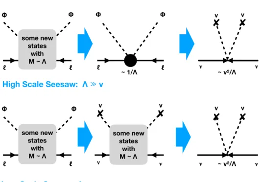
ν =−v2c[5]Λ−1. Herev = 174 GeV is the Higgs field expectation value and c[5]Λ−1 is some flavour matrix of dimension 1/mass. The dimension-5 operator (10) is not renormalisable; in an effective field theory approach it can be understood as the low energy limit of renormalisable operators that is obtained after ”integrating out” heavier degrees of freedom, see Fig. 1. The Majorana mass term (9) can be diagonalised by a transformation
mν =Uνdiag(m1, m2, m3)UνT. (11)
2.3. Neutrino mass and New Physics
The previous considerations show that the explanation of neutrino masses within the framework of renormalisable relativistic quantum field theory certainly requires adding new degrees of freedom to the SM. Leaving aside the somewhat boring possibility of Dirac neu-trinos discussed after Eq. (8),11 this implies the existence of new particles. Hence, neutrino
masses may act as a ”portal” to a (possibly more complicated) unknown/hidden sector that may yield the answer to deep questions in cosmology, such as the origin of matter and DM. There are different possible explanations why these new particles have not been found. One possibility is that their masses are larger than the energy of collisions at the LHC. Another
10This is in contrast to all SM particles, for which such a term is forbidden by gauge symmetry unless it
is generated by a spontaneous symmetry breaking.
11It should be emphasised that there exist more interesting ways to generate Dirac neutrinos than simply
some new states
with M ~ Λ
Φ
Φ Φ Φ
~ 1/Λ ℓ
ℓ ℓ ℓ
~ v²/Λ v v
ν ν
some new states
with M ~ Λ
Φ Φ
ℓ ℓ
v v
~ v²/Λ
ν ν
some new states
with M ~ Λ
ν ν
v v
High Scale Seesaw: Λ
≫
vLow Scale Seesaw: Λ
≲
vFigure 1: If the new states associated with neutrino mass generation are much heavier than the energies E in an experiment (ΛE), then they do not propagate as real particles in processes, and the Feynman diagram on the left can in good approximation be replaced by a local “contact interaction” vertex that we e.g. represent by the black dot in the diagram in the middle in the first row. This is analogous to the way the four fermion interaction ∝GF in Fermi’s theory is obtained from integrating out the weak gauge
bosons. In high scale seesaw models (Λ v mi, upper row in the figure) this description holds for
all laboratory experiments. At energiesE v, there are no real Higgs particles, and one can replace the Higgs field by its expectation value, Φ→(0, v)T. Then the operator (10) reduces to the mass term (9) with mν =−v2c[5]Λ−1, which can be represented by the diagram on the right. Here the dashed Higgs lines that
end in a cross represent the insertion of a Higgs vev v. They and the effective vertex are often omitted, so that the Majorana mass term is simply represented by “clashing arrows”. In low scale seesaw models (v >Λmi, cf. sec.2.4.2) the order of the two steps (in terms of energy scales) is reversed, as illustrated
possibility is that the new particles couple only feebly to ordinary matter, leading to tiny branching ratios.
Any model of neutrino masses should explain the “mass puzzle”, i.e. the fact that the mi are many orders of magnitude smaller than any other fermion masses in the SM. A key unknown is the energy scale Λ of the New Physics that is primarily responsible for the neutrino mass generation. Typically (though not necessarily) one expects the new particles to have masses of this order,12 and we assume this in the following. The fact that current
neutrino oscillation data is consistent with the minimal hypothesis of three light neutrino mass eigenstates suggests that Λ is much larger than the typical energy of neutrino oscillation experiments,13 so that neutrino oscillations can be described in the framework of Effective Field Theory (EFT) in terms of operators O[in] = ci[n]Λn−4 of mass dimension n > 4 that
are suppressed by powers of Λn−4. Here the c[n]
i are flavour matrices of so-called Wilson coefficients. If the underlying theory is required to preserve unitarity at the perturbative level, Λ should be below the Planck scale [60]. The only operator with n = 5 is given by eq. (10). The smallness of the mi can then be explained by one or several of the following reasons: a) Λ is large, b) the entries of the matricesc[in] are small, c) there are cancellations between different terms inmν.
a) High scale seesaw mechanism: Values of Λ v far above the electroweak scale automatically lead to smallmi, which has earned this idea the nameseesaw mechanism (”as Λ goes up, the mi go down”). The three tree level implementations of the seesaw idea [61] are known as type-I [62–67] type-II [67–71] and type-III [72] seesaw. The type I seesaw is the extension of the SM byn right handed neutrinos νRi with Yukawa couplings `LF νRΦ and a Majorana mass˜ νRMMνRc (hence Λ ∼ MM). It is discussed below in 2.4 and gives rise to the operator (10) with c[5]Λ−1 = F M−1
M FT, cf. (13). In the type-II seesaw, mν is directly generated by an additional Higgs field ∆ that transforms as a SU(2) triplet, while the type-III mechanism involves a fermionic SU(2) triplet ΣL.
b) Small numbers: The mi can be made small for any value of Λ if the Wilson coeffi-cientsc[in]are small, which can be explained in different ways. One possibility is that it is the consequence of a small coupling constant. The Dirac neutrino scenario discussed below Eq. (8) is of this kind. A popular way of introducing very small coupling
con-12 Light (pseudo) Goldstone degrees of freedom can e.g. appear if the smallness of neutrino masses is
caused be an approximate symmetry. Moreover, some dimensionful quantities (e.g. the expectation value of a symmetry breaking field) can take very small values while the masses of the associated particles remain well above the energy scale of neutrino oscillation experiments.
13Several comments are in place here. First, while the good agreement of the three light neutrino picture
with data clearly suggests that Λ eV, this is not a necessity, cf. e.g. [58]. Moreover, while the lack of evidence for deviations η from unitarity in Vν or exotic signatures in the near detectors of neutrino
stants without tuning them ”by hand” is to assume that they are created due to the spontaneous symmetry breaking of a flavour symmetry by one or several flavons [73]. This may also help to address the flavour puzzle. Small c[in] can further be justified if the Oi[n] are generated radiatively, cf. e.g. [74–78] and many subsequent works. The suppression due to the “loop factor” (4π)2 alone is not sufficient to explain the
small-ness of themi, and the decisive factor is usually the suppression due to a small coupling of the new particles in the loop, possibly accompanied by a seesaw-like suppression due to the heavy masses of the particles in the loop. More exotic explanations e.g. involve extra dimensions [79,80], string effects [81, 82] or the gravitational anomaly [83].
c) Protecting symmetry: The physical neutrino mass squares m2
i are given by the eigenvalues of m†νmν. Individual entries of the light neutrino mass matrix mν are not directly constrained by neutrino oscillation experiments and may be much larger than themi if there is a symmetry that leads to cancellations inm†νmν. These cancellations can either be ”accidental” (which often requires come fine-tuning) or may be explained by an approximate global symmetry. A comparably low New Physics scale can e.g. be made consistent with small mi in a natural way if a generalised B-L symmetry is approximately conserved by the New Physics. Popular models that can implement this idea include the inverse [84–86] and linear [87, 88] seesaw, scale invariant models [89] and theνMSM [90].14
Of course, any combination of these concepts may be realised in nature, including the simul-taneous presence of different seesaw mechanisms. For instance, a combination of moderately large Λ∼TeV and moderately small Yukawa couplingsF ∼10−5(similar to that of the
elec-tron) is sufficient to generate a viable low scale type-I seesaw mechanism without the need of any protecting symmetry. If a protecting symmetry as added, a TeV scale seesaw is feasible with O[1] Yukawa couplings or, alternatively, even values of Λ below the electroweak scale can explain the observed neutrino oscillations in a technically natural way [90]. Models with Λ at or below the TeV scale are commonly referred to aslow scale seesaw cf. sec.2.4.2. The typical seesaw behaviour thatmi decreases if Λ is increased holds in such scenarios as long as Λmi, in spite of the fact thatv/Λ is not a small quantity. The EFT treatment in terms of Oi[n] may still hold for neutrino oscillation experiments, but the collider phenomenology of low scale seesaw models [94] has to be studied in the full theory if Λ is near or below the collision energy, cf. fig. 1.
In addition to the smallness of the neutrino masses, it is desirable to find an explanation for the “flavour puzzle”, i.e., the observed mixing pattern of neutrinos. Numerous attempts have been made to identify discrete or continuous symmetries inmν. An overview of scenarios
that are relevant in the context of sterile neutrino DM is e.g. given in Ref. [95]. The basic problem is that the reservoir of possible symmetries to choose from is practically unlimited. For any possible observed pattern of neutrino masses and mixings one can find a symmetry that “predicts” it. Models can only be convincing if they either predict observables that have not been measured at the time when they were proposed, such as sum rules for the mass [95–99] or mixing [95,100–102], or are “simple” and aesthetically appealing from some (subjective) viewpoint. Prior to the measurement ofθ13, models predictingθ13= 0 appeared
very well-motivated, such as those with tri/bi-maximal mixing [103–107]. The observed θ136= 0, however, makes it difficult to explain mν in terms of a simple symmetry and a small number of parameters, as the number of parameters that have to be introduced to break the underlying symmetries is usually comparable to or even larger than the number of free parameters in mν that one wants to explain. An interesting alternative way to look at this is to compare the predictivity of different models to the possibility that the values inmν are simply random [108].
2.4. Sterile Neutrinos
2.4.1. Right Handed Neutrinos and Type-I Seesaw
The terms ”sterile neutrino”, ”right handed neutrino”, ”heavy neutral lepton” and ”sin-glet fermion” are often used interchangeably in the literature. In what follows we apply the term “sterile neutrino” to singlet fermions that mix with the neutrinos νL, i.e., we consider this mixing as a defining feature that distinguishes a sterile neutrino from a generic singlet fermion. Such particles are predicted by many extensions of the SM, and in particular in the type-I seesaw model, which is defined by adding n RH neutrinos νR to the SM. The Lagrangian reads15
L =LSM+i νRi6∂νRi−
1 2
νRic (MM)ijνRj+νRi(MM† )ijνRjc
−Fai`Laεφ∗νRi−Fai∗νRiφTε†`La . (12)
LSM is the Lagrangian of the SM. The Fai are Yukawa couplings between the νRi, the Higgs field φand the SM leptons`a. Here we have suppressed SU(2) indices; ε is the totally antisymmetric SU(2) tensor. MM is a Majorana mass matrix for the singlet fields νRi. The Majorana mass term MM is allowed for νR because the νR are gauge singlets. The lowest New Physics scale Λ should here be identified with the smallest of the eigenvaluesMI (with I = 1, . . . n) of MM. At energiesE Λ, theνR can be “integrated out” and (12) effectively reduces to
Leff = LSM+
1 2
¯
`LΦF M˜ M−1F TΦ˜T`c
L (13)
and thus generates the term (10) with c[5]Λ−1 =F M−1
M FT. The Higgs mechanism generates the Majorana mass term (9) from (13), and mν is given by
mν =−v2F MM−1FT, (14)
15Here we represent the fields with left and right chirality by four component spinors ν
L and νR with
where v = 174 GeV is the Higgs field expectation value. The full neutrino mass term after electroweak symmetry breaking reads
1 2(νL ν
c R)M
νc
L νR
+h.c.≡ 1
2(νL ν c R)
0 mD
mT
D MM
νc L νR
+h.c., (15)
where mD ≡ F v. The magnitude of the MI is experimentally almost unconstrained, and different choices have very different implications for particle physics, cosmology and astro-physics, see e.g. [30] for a review. For MI 1 eV there is a hierarchy mD MM (in terms of eigenvalues), and one finds two distinct sets of mass eigenstates: Three light neutrinos νi that can be identified with the known neutrinos, and n states that have masses ∼ MI. Mixing between the active and sterile neutrinos is suppressed by elements of the mixing matrix
θ ≡mDMM−1. (16)
This allows to rewrite (14) as
mν =−v2F MM−1F
T =−m
DMM−1m T
D =−θMMθT. (17)
All 3 +n mass eigenstates are Majorana fermions and can be represented by the elements of the flavour vectors16
ν=Vν†νL−Uν†θνRc +VνTνLc −UνTθ
∗
νR (18)
and
N =VN†νR+ ΘTνLc +V T Nν
c R+ Θ
†
νL, (19)
The unitary matrices Uν and UN diagonalise the mass matrices mν and MN ≡ MM +
1 2 θ
†θM
M+MMTθTθ
∗
of the light and heavy neutrinos, respectively, as MNdiag =UT
NMNUN = diag(M1, M2, M3) andmdiagν =Uν†mνUν∗ = diag(m1, m2, m3). The eigenvalues ofMM andMN coincide in good approximation, we do not distinguish them in what follows and refer to both as MI. The light neutrino mixing matrix in Eq. (4) and its heavy equivalent VN are given by
Vν ≡
I− 1 2θθ
†
Uν andVN ≡
I− 1 2θ
Tθ∗
UN, (20)
16 In principle there is no qualitative difference between the mass states ν
i and NI, the difference is a
quantitative one in terms of the values of the masses and mixing angles. One could simply use a single index i = 1. . .3 +n and refer to NI as νi=3+I, with mass mi=3+I = MI. This is indeed often done in
and comparison with (5) reveals η = −1 2θθ
†.17 The active-sterile mixing is determined
by the matrix
Θ≡θUN∗. (21)
An important implication of the relation (17) is that one NI with non-vanishing mixing θαI is needed for each non-zero light neutrino mass mi. Hence, if the minimal seesaw mech-anism is the only source of light neutrino masses, there must be at leastn = 2 RH neutrinos because two mass splittings ∆msol and ∆matm have been observed. If the lightest neutrino
is massive, i.e. mlightest≡min(m1, m2, m3)6= 0, then this implies n ≥3, irrespectively of the
magnitude of the MI. A heavy neutrino that is a DM candidate (let us call it N1) would
not count in this context [110]: to ensure its longevity, the three mixing angles θα1 must
be so tiny that their effect on the light neutrino masses in Eq. (17) is negligible. This has an interesting consequence for the scenario in which the number n of sterile flavours equals the number of generations in the SM (n = 3): If one of the heavy neutrinos composes the DM, then the lightest neutrino is effectively massless (mlightest ' 0). If, on the other hand,
mlightest >10−3 eV, then all NI must have sizeable mixings θαI, which implies that they are
too short lived to be the DM , cf. Eq. (29). These conclusions can of course be avoided for n >3, or if there is another source of neutrino mass.
2.4.2. Low Scale Seesaw
In conventional seesaw models, it is assumed that the scale Λ is not only larger than the mi, but even much larger than the electroweak scale. This hierarchy is suggested in Eq. (13). In this case the smallness of the mi is basically a result of the smallness of v/Λ or, more precisely, v/MI 1. If they are produced via the weak interactions of their θαI -suppressed components νLα, then heavy neutrinos NI that compose the DM usually must have masses below the electroweak scale (MI < v). Otherwise the upper bound on the magnitude of theθαI from the requirement that their lifetime exceeds the age of the universe prohibits an efficient thermal production in the early universe. MM therefore has at least one eigenvalue below the electroweak scale in such scenarios. A particular motivation for so-called low scale seesaws comes from the fact that they avoid the hierarchy problem due to contributions from superheavy NI to the Higgs mass [111]. Moreover, the fact that the properties of the Higgs boson and top quark appear to be precisely in the narrow regime where the electroweak vacuum is metastable [112] and a vacuum decay catastrophe [113] can be avoided may suggest the absence of any new scale between the electroweak and Planck scale [114, 115].
Popular low scale seesaw scenarios include the inverse [84–86] and linear [87, 88] seesaw, the νMSM [90] and scenarios based on on classical scale invariance [89]. They often involve some implementation of a generalisedB−Lsymmetry, and the smallness of the light neutrino masses mi is explained as a result of the smallness of the symmetry breaking parameters (rather thanv/MI). Sterile neutrino DM candidates can be motivated in the minimal model
17Unfortunately, unitarity violation due to heavy neutrinos does not appear to be able to resolve the
(12) [36,90] as well as various different extensions, cf. ref. [43,116] for reviews and e.g. refs. [117–120] for specific examples.
For n = 3, and in the basis where MM and the charged lepton Yukawa couplings are diagonal in flavour space, one can express MM and F as
MM = Λ
µ0 0 0
0 1−µ 0
0 0 1 +µ
, F =
0e Fe+e i(Fe−e) 0µ Fµ+µ i(Fµ−µ) 0τ Fτ+τ i(Fτ −τ)
(22)
without any loss of generality. Here Λ is the characteristic seesaw scale, the Fα are generic Yukawa couplings and the dimensionless quantities α, 0α, µ, µ0 are symmetry breaking pa-rameters. In the limitα, 0α, µ, µ
0 →0 the quantityB−L¯ is conserved, where the generalised
lepton number
¯
L=L+LνR (23)
is composed of the SM lepton number L and a charge LνR that can be associated with
the right handed neutrinos in the symmetric limit; the combination √1
2(νR2+iνR3) carries
LνR = 1, the combination
1
√
2(νR2 −iνR3) carries LνR = −1 and νR1 carries LνR = 0. Such
scenarios can provide a sterile neutrino DM candidate (hereN1) in a technically natural way:
The smallness of µ0explains its low mass, while the small of the 0α can ensure its longevity. Recent reviews of models including keV sterile neutrinos can e.g. be found in refs. [43,116]. The parametrisation (22) is completely general; specific models can make predictions how exactly the limit α, 0α, µ, µ
0 →0 should be taken.
An appealing feature of low scale scenarios is that the heavy neutrinos can be searched for experimentally in fixed target experiments [121] like SHiP [122, 123] or NA62 [124,125], at the existing [126–131] or future [132–135] LHC experiments or at future colliders [136–138]. Observable event rates
[90, 139, 140]. The interactions of the light and heavy neutrinos can be determined by inserting the relation νL = PL(Vνν+ ΘN) from eq. (18) into eq. (3). The unitarity viola-tion in Vν implies a flavour-dependent suppression of the light neutrinos’ weak interactions Eq. (18). The NI haveθ-suppressed weak interactions [141–143] due to the doublet compo-nent ΘT
IανLαc + Θ
†
IανLα in (18). In addition, the NI directly couple to the Higgs boson via their Yukawa coupling to the physical Higgs field h in (12) in unitary gauge. The full NI interaction term at leading order in θ can be expressed as
L ⊃ − √g
2NΘ
†
γµeLWµ+− g
√
2eLγ
µΘN W−
µ
− g
2 cosθWNΘ
†
γµνLZµ− g
2 cosθWνLγ
µΘN Z µ
− √g
2 MN mW
ΘhνLN −√g
2 MN mW
Θ†hN νL . (24)
DM sterile neutrinos because the tiny mixing angle that is required to ensure their stability on cosmological time scales implies that the branching ratios are too small. We discuss dedicated experimental searches for DM sterile neutrinos in Sec. 5.
2.4.3. The Neutrino Minimal Standard Model
Since all of the problems I)-IV) summarised in sec.1.2should be explained in a consistent extension of the SM, it is instructive to address them together. One possible guideline in the search for a common solution is provided by the “Ockham’s razor” approach, which has been highly successful in science in the past: one tries to minimise the number of new entities introduced but maximise the number of problems which can be addressed simultaneously. A specific low scale seesaw model that realises this idea was suggested in 2005 [36, 37], see [146] for a review. This Neutrino Minimal Standard Model (νMSM) provides a new systematic approach that addresses the beyond-the-Standard-Model problems in a bottom-up fashion, not introducing particle heavier than the Higgs boson and attempting to be complete [114, 151] and testable [121, 136, 138, 152–154]. In this approach the three right-handed neutrinos are responsible for neutrino flavour oscillations, generate the BAU via low scale leptogenesis [37, 155] and provide a DM candidate. The DM candidate has a keV mass and very feeble interactions, while the other two have quasi-degenerate masses between
∼ 100 MeV and the electroweak scale; these particles are responsible for the generation of light neutrino masses and baryogenesis. This os precisely the pattern predicted by eq. (22) if all symmetry breaking parameters are small. The feasibility of this scenario was proven with a parameter space study in Refs. [156,157]. In theνMSM the interactions of the DM particles with the Standard model sector are so feeble that these particles never enter the equilibrium with primordial plasma and therefore their number density is greatly reduced (as compared to those of neutrinos). In this way they evade the combination of Tremain-Gunn [21] and cosmological bounds.
3. Properties of Sterile Neutrino Dark Matter
As originally suggested in [31], sterile neutrinos with the mass in the keV range can play the role of DM.18 Indeed, these particles are neutral, massive and, while unstable, can have
their lifetime longer than the age of the Universe (controlled by the active-sterile mixing pa-rameterθ).19 Such sterile neutrinos are produced in the early Universe at high temperatures.
18In this section we almost exclusively focus on the minimal scenario where sterile neutrino DM is produced
thermally via theθ-suppressed weak interactions, which favours the keV scale due to constraints onθcoming from X-ray observations discussed further below. If the DM is produced via another mechanism which does not rely on this mixing, cf. sec.4, then there is no lower bound on the|θαI|and X-ray constraints can be
avoided by making them arbitrarily small. This means that the DM particles can be much heavier than keV. However, while these are perfectly viable models of singlet fermion DM, they do not fall under our definition ofsterile neutrinos because the new particles practically do not mix with the SM neutrinos, cf. sec.2.4.
19In this section we consider the case of one sterile neutrinoN with massM and mixingsθ
αwith the SM
Unlike other cosmic relic particles (e.g. photons, neutrinos or hypothetical WIMPs) the feeble interaction strength of sterile neutrinos means that they were never in thermal equilibrium in the early Universe and that their exact production mechanism is model-dependent (see Section4). In the following we discuss the most important observational constraints on these particles as DM candidates. These can broadly be classified into three main categories,
• the phase space density in DM dense objects, cf. sec.3.1,
• indirect detection through emission from the decay of sterile neutrino DM, cf. sec.3.2,
• the effect of their free streaming on the formation of structures in the universe, cf. sec. 3.3.
A selection of constraints is summarised in sec. 3.4.
3.1. Phase Space Considerations
Being out of equilibrium implies nN nν for the number densitynN of sterile neutrinos, where the number of relic neutrinos, nν, is given by Eq. (1). As a result, the observed DM densityρDM =M nN can be achieved with the mass of DM particles that satisfy (even satu-rate) the lower bound for the fermionic DM, the Tremaine-Gunn bound [21], assuming that the phase-space density of DM particles in a galaxy does not exceed that of the degenerate Fermi gas. The strongest lower bound comes from the dwarf spheroidal satellites of the Milky way (dSph) and is O(100) eV. We do not quote the exact numerical value, as it depends on the set of dSphs used, and on the way to estimate the phase-space density of DM particles based on the observational data (for the discussion see [22,158–160]). Assuming a particular primordial phase-space distribution of DM particles that obeys the Liouville theorem in the process of evolution, one may additionally strengthen the bounds [22] (see also [161] where the several newly-discovered satellite galaxies from wide-field optical surveys such as the Dark Energy Survey (DES) and Pan-STARRS were included). A pedagogical review of this argument is given e.g. in [22] or in [43, Section 4.1].20
3.2. Decaying Dark Matter 3.2.1. Existing Constraints
For sterile neutrino masses below twice the value of the electron mass the dominant decay channel is N → νανβν¯β (all possible combinations of flavours are allowed, including charge conjugated decay channels as N is a Majorana particle). The total decay width N → 3ν is given by [165, 166]
ΓN→3ν = G2
FM5 96π3
X
α
|θα|2 ≈ 1
1.5×10¹⁴sec
M 10 keV
5 X
α
|θα|2 (25)
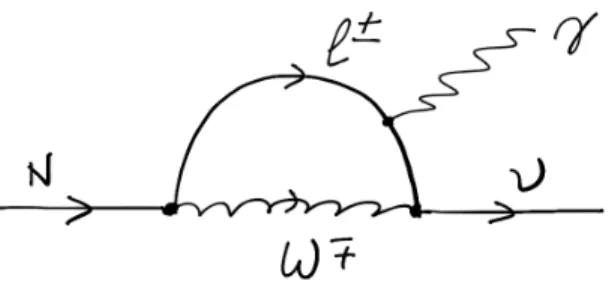
Figure 2: Radiative decay of sterile neutrinoN→γ+να. A similar diagram where a photon couples to the
W-boson is not shown. TheN coupling to weak gauge bosons exists for each flavour and is proportional to θα, cf. (24).
From now on we will discuss the total mixing angle and use the simplified notation
θ2 ≡ X
α=e,µ,τ
|θα|2, (26)
within this section, not to be confused with the full mixing matrixθ in eq. (16) and following. If one requires that the lifetime corresponding to the process (25) should be (much) longer than the age of the Universe,tUniverse = 4.4×10¹⁷sec [18] the bound on the sum of the mixing
angles θ2
α becomes (see Fig. 14)
θ2 <3.3×10⁻⁴
10 keV M
5
— lifetime longer than the age of the Universe (27)
Already the requirement that the sterile neutrino lifetime is longer than the age of the Universe (bound (27)) implies that the contribution of DM sterile neutrino to the neutrino masses,δmν ∼M θ2, is smaller than the solar neutrino mass differencemsol= 0.0086 eV) [36,
110]. Therefore, at least two more sterile neutrinos are required to explain to observed mass differences, as discussed already in 2.4. If the neutrino masses are due to exactly two sterile neutrinos, the lightest active mass eigenstate, m1 is essentially zero, which bounds the total
sum of neutrino masses to be
X
i
mi 'κmatm (28)
where κ = 1 for the case of normal hierarchy and κ = 2 for the case of inverted hierarchy. This is a non-trivial prediction that can be checked by ESA’s Euclid space mission [167].
Along with the dominant decay channel, N → 3ν sterile neutrino also possesses a loop mediated radiative decay N →ν+γ [165] (Fig. 2). The decay width of this process is [165,
166]
ΓN→γν =
9α G2
F 256π4 θ
2M5 = 5.5×10⁻²²θ2
M 1 keV
5
sec−1 . (29)
While it is suppressed by 278πα ≈ 1
128 as compared to the main decay channel, such a decay
4x101 4x10³
1x10² 1x10³
2 4 6 8 10 12 14 16 18 20
10 20 30 40 50 60 70 80
DM column density [M
Sun
/pc
2 ]
Off-center distance [kpc] Off-center distance [arcmin]
Widrow Dubinski (2005), M31B Chemin et al. (2009), ISO
Corbelli et al. (2009), rB = 28 kpc Maximum disk, Kerins et al.’00
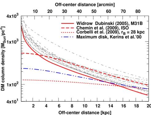
Figure 3: DM column density (DM density distributions, integrated along the line of sight) for different DM density profiles of Andromeda galaxy (M31). The profiles used are [170–176]. The extreme profiles of
Corbelli et al.[174] andKerins et al.[176] are unphysical but demonstrate how much matter can be “pushed” into baryonic, rather than DM mass.
the DM, then such a mono-chromatic signal is potentially detectable from spots on the sky with large DM overdensities [34,41,168]. This opens an exciting possibility of astrophysical searches of sterile neutrino DM.
The number of photons from DM decay is proportional to the DM column density – integral of the DM distribution along the line of sight (l.o.s.):
S = Z
l.o.s.
ρDM(r)dr (30)
Averaged over a sufficiently large field-of-view (of the order of 100 or more) this integral becomes only weakly sensitive to the underlying DM distributions (see, e.g. Fig. 3 where this is illustrated for the case of Andromeda galaxy, based on [169]).21
As a result a vast variety of astrophysical objects of different nature would produce a comparable decay signal [40,177, 178]. Therefore,
• one has a freedom of choosing the observational targets, avoiding complicated astro-physical backgrounds;
21The same scatter in the DM density profiles gives a much larger uncertainty in the annihilationJ-factor
• if a candidate line is found, its surface brightness profile may be measured, distinguished from astrophysical lines (which usually decay in outskirts) and compared among several objects with the same expected signal.
In this way one can efficiently distinguish the decaying DM line from astrophysical back-grounds.
Searches of this decaying DM signal in the keV–MeV mass range have been conducted using a wide range of X-ray telescopes: XMM-Newton [39, 40, 179–190], Chandra [169,
191–199], Suzaku [183, 200–203], Swift [204], INTEGRAL [205, 206], HEAO-1 [39] and Fermi/GBM [207, 208], as well as a rocket-borne X-ray microcalorimeter [209–211], NuS-tar [212–214] (we use a more conservative of two NuStar bounds [213] and [214] for our final summary plot in Section 6). The bounds from the non-observation of DM decay line in X-rays discussed in more detail in Refs.[43, 215].
3.2.2. Status of the 3.5 keV Line
Recently, an unidentified feature in the X-ray spectra of galaxy clusters [184, 188] as well as Andromeda [188] and the Milky Way galaxies [187] have been reported by two independent groups. The signal can be interpreted as coming from the decay of a DM particle with the mass ∼ 7 keV (in particular of a sterile neutrino with the mixing angle sin22θ ' (0.2− 2)×10−10). The signal sparked a great deal of interest. A number of
works have subsequently found the line in the spectra of galaxies clusters [186, 201, 216] or galaxies [185, 213, 214, 217]). Other DM-dominated objects did not reveal the presence of the line [198, 202, 203, 211, 212, 218, 219]. Possible explanations of the origin of the line also included: statistical fluctuation, unknown astrophysical line; an instrumental feature.
Statistical fluctuation? The original detections were at the level 3−4σ. By now the line has been observed in the spectra of many objects, with its formal statistical significance exceeding 5σ [184, 187, 188] (even taking into account the “look elsewhere effect” ). The intensity of the line is consistent with the estimates of DM column density [185, 187, 216]. So, while in some object the line can be just a fluctuation “in the right position”, this cannot be the only explanation of its origin. Recent observation of the line at 11σ in the blank sky dataset with the NuStar satellite [213] made the “statistical fluctuation” even less likely.22
An unknown instrumental effect (systematics)? Given high statistical power of the datasets (with the statistical errors being 1% or less) a natural “suspect” would be a systematics of the instrument (for example, a per-cent level unknown feature in the effective area of the telescope would explain such a “bump” in the spectrum). However, many works have demonstrated that such an explanation does not hold. First of all, the line was shown to scale correctly with the redshift of the source (see [184, 188, 216]) which is impossible to explain with any feature related to the instrument. In addition, the line has been observed by 4 instruments. Therefore any explanation should appeal to instrumental featurecommon
in all 4 telescopes. In particular. the presence of the Au M-absorption edge at energy
∼3.4249 keV [221,222], invoked as a reason for explaining the feature inXMM-Newton and Suzaku would not explain the feature in the spectra observed with Chandra [217] (where Iridium is used instead of Gold [223]) or inNuStar [213,214] (where observations are based on “bounce-0” (stray) photons not collected by the mirrors). In addition, the systematics related to the properties of CCD detector (common inXMM-Newton,Chandra, andSuzaku) would not explain the feature in the spectrum of NuStar with its Cadmium-Zinc-Telluride detectors. Finally, an 11σ detection of the 3.5 keV signal by NuStar from a quiescent region of the sky [213] and a subsequent confirmation of this result with the Chandra X-ray observatory [217] suggest that the line is not a statistical fluctuation and nor an artefact of the XMM-Newton’s instrumentation.
Atomic transition as the origin of the line? It was argued that the line could originated from atomic transition (e.g. Potassium XVIII with lines at 3.47 and 3.51 keV [198,
224–226] or Charge Exchange between neutral Hydrogen and bare sulphur ions leading to the enhanced transitions between highly excited states and ground states of S XVI [227–
229]. The corresponding sulphur transitions have energies in the range 3.4−3.45 keV – close to the nominal position of the detected line (for further discussion see [189, 217, 230, 231] or [43]). It should be noted that the spectral resolution ofXMM-Newton (as well as Suzaku, Chandra or NuStar) does not allow to resolve the intrinsic width of the lines (or separate lines of the multiplet of K XVIII).
Recently the centre of the Perseus galaxy cluster has been observed with the Hitomi spectrometer [232] whose energy resolution at energies of interest is few eV. The observation did not reveal any atomic lines around 3.5 keV (and only minor residuals at 3.4−3.45 keV that could be interpreted as S XVII charge exchange, insufficient to account for a strong signal
from the centre of the Perseus cluster, as found byXMM-Newton andSuzaku [184,186,201]. While these observations rule out atomic transitions as the origin of 3.5 keV line, they leave room for DM interpretation. Indeed, typical broadening of the atomic lines in the centre of the Perseus cluster are determined by thermal and turbulent motions and correspond go the width vtherm ∼ 180 km/sec [232]. The width of a DM decay line, on the other hand, is determined by the virial velocity that is of the order vvir ∼ 1300 km/sec [233]. The corresponding Doppler broadening is wider than the spectral resolution of the Hitomi spectrometer and therefore the bounds on the putative DM decay line are much weaker than the limit on the astrophysical line. As a result the bounds of Hitomi are consistent with XMM-Newton detection in galaxies and galaxy clusters.
Future progress with our understanding of the nature of 3.5 keV line will come with the next generation of high-resolution X-ray missions, including XARM (Hitomi replace-ment mission)23, LYNX24 and Athena+ [234]. Additionally, microcalorimeters on sounding rockets [211] looking into the direction of Galactic Centre may confirm the origin of the line.
23https://heasarc.gsfc.nasa.gov/docs/xarm
3.3. Sterile Neutrinos and Structure Formation
All production mechanisms discussed in Section 4 tend to predict non-thermal sterile neutrino momentum distributions that potentially exhibit a non-negligible free streaming length in the early universe and will thereby affect the formation of structures in the early universe. In the following we review the observational constraints on the free streaming in a mostly model-independent manner. The conversion of these results into constraints on the mass and mixing of sterile neutrinos is highly model dependent, and there are still considerable uncertainties in different aspects of the problem (including the production in the early universe, the simulation of non-linear structure formation as well as the difficulty to observe small scale structures). Here we mostly focus on the (non-resonant or resonant) thermal production mechanism described in Section 4.2 as an example.25
3.3.1. Warm Dark Matter
The production of sterile neutrinos occurs at temperatures much higher than the de-coupling temperature of active neutrinos, Tdec ∼ 1 MeV. Therefore, for masses in the keV range sterile neutrino particles are bornrelativistic. DM candidates with such properties are commonly referred to as Warm Dark Matter (or WDM).26 The original idea of WDM dates back to 1980s and was revitalised from mid-1990s onward (largely due to the idea of sterile neutrino DM [31, 237]). It is very difficult to give proper credits, for an incomplete list of early papers see e.g. [31–33, 237–245].
Warm DM particles change the formation of structures in the Universe as compared to the cold DM case. While DM particles are still relativistic, they do not cluster, but rather stream freely. This erases primordial density perturbations at scales below their free-streaming horizon (usually called simplyfree streaming scale, see [246] for discussion of some subtleties and confusions associated with the definitions). This quantity is defined in the usual way:
λfs(t)≡a(t)
Z t
ti
dt0 v(t
0)
a(t0) ≈1 Mpc
keV M
hpDMi
hpνi
(31)
(see [246] for details). Here v(t) is a typical velocity of DM particles, ti is the initial time (its particular value plays no role); a(t) is the scale factor as a function of (physical) time. In the last equality, hpDMi and hpνi are the average absolute values of momentum of DM particles and active neutrinos. The integral is saturated at early times when DM particles are relativistic (v(t)≈1).
The free-streaming horizon indicates at what scales matter power spectrum of warm DM particles will be distinguishable from that of CDM.The scales affected by the keV-scale warm DM are Mpc or below.
25 The other mechanisms have also been studied in detail in the literature, recent results and references
can e.g. be found in Refs. [43, 235,236].
26 Following common convention, we use the term WDM for particles that are relativistic when they are
0 2 4 6 8 q [=p/Tν]
10−5 10−4 10−3 10−2 q 2f(q)
L6= 0.0
1.0 2.0 4.0 6.0 8.0 10.0 16.0 20.0 50.0 120.0 700.0
Ms=7keV
×102
0.1 1.0 10.0 100.0
k [h Mpc−1]
1 10 100 1000 k 3P(k) CDM 0.0 1.0 2.0 4.0 6.0 8.0 10.0 16.0 20.0 50.0 120.0 700.0
Mth=1.4 keV
Ms=7 keV
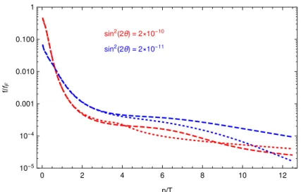
Figure 4: Sterile neutrino DM vs. thermal relics. Left: Sterile neutrino momentum distributions for different values ofL6, the lepton asymmetry in units of 10−6, withL6= [0,700] as indicated by the legend. Each distributionf(q) is multiplied by the momentum squared,q2×f(q), to reduce the dynamic range. Solid black line – the Fermi-Dirac distribution of a thermal relic with the massMth= 1.4 keV (the temperature of this distribution is different fromTν). Dashed black line – Fermi-Dirac distribution withT =Tν, multiplied
by 10−2 to fit into the plot. The momenta are plotted for the thermal plasma at a temperature of 1 MeV. The sterile neutrino mass is 7 keV. Right: Matter power spectra generated from the 7 keV distribution functions shown in the left panel. The CDM power spectrum is shown as a solid black line. The dashed line corresponds to the power spectrum of a thermal relic of mass 1.4 keV, which is the thermal relic counterpart of the non-resonantly produced 7 keV sterile neutrino. From [248].
Historically the first warm DM candidates were heavier analogues of neutrinos – particles that decoupled from the equilibrium with primordial plasma while being relativistic. To reconcile their mass with the Tremaine-Gunn bound, discussed above, such particles – known as relativistic thermal relics – needed to decouple much earlier than the ordinary neutrinos and one had to arrange for a significant entropy dilution that would reduce the number density of the thermal relics, ntr nν, thus reconciling astrophysical and cosmological DM observables. For thermal relics the suppression of power spectrum at small scales (large comoving k) behaves as k−10 [245, 247]. This scale can be directly related to the
free-streaming (31) (see [246]).
The situation is different for sterile neutrino DM produced via non-resonant [31, 35, 38,
249] or resonant [32, 250–252] mixing with active neutrinos, cf sec. 4.2. These particles are produced out of thermal equilibrium (see Section 4) and therefore there is no universal be-haviour of their primordial velocity spectrum, Fig.4. As a result primordial power spectrum depends on the whole primordial momentum distribution function (see Fig.4). In particular, the small scale behaviour of the matter power spectra differs drastically even for the particles of the same mass. The power spectra of sterile neutrino DM can be roughly approximated as a mixture of cold and warm components [253].
1. Measure the matter power spectrum at relevant scales (Lyman-α forest; weak lensing; 21 cm line). We discuss the Lyman-α forest in Section3.3.2 and comment very briefly on the other methods.
2. Determine the number of collapsed structures as a function of their masses and redshifts (dwarf galaxy counts; reionisation history; collapsed objects at high-z Universe). We discuss some of these approaches and their limitations in Section 3.3.4.
3. Determine the distribution of matter within individual DM dominated objects (cores in galactic halos). We shall not discuss this question in the current review and refer an interested reader to [43, Section 3.3].
Below we will discuss the most powerful methods, and overview the other ones briefly.
3.3.2. Lyman-α Forest Method
The power spectrum of matter at scales ∼ 0.1–1 Mpc and redshifts z = 2−6 can be determined by the so-called Lyman-α forest method [254–258].
At these redshifts large fraction of primordial hydrogen fills a network of mildly non-linear structures (filaments), forming the so-called intergalactic medium (IGM). The hydro-gen makes filaments “visible” via absorption features in the spectra of distant quasars. The statistics of these absorption features allows to reconstruct the distribution of neutral hy-drogen and, under the assumption that it traces the matter distribution, the matter power spectrum itself [254–258]. The structure of the filaments is different in cold- and warm DM cosmologies [259–261] which makes Lyman-α forest method a powerful probe of DM free-streaming [53, 246, 247, 253, 262–270].
The basic observable of the method is the one-dimensionalflux power spectrum– a Fourier transform of the transmitted flux correlation function averaged along the lines of sight. It is not possible to de-project this observable and to reconstruct the underlying matter power spectrum [271]. Therefore the common approach is to compare the data to the mock spectra extracted from hydrodynamical simulations. Extraction and analysis process attempts to closely replicate the physics of real experiments, in particular, taking into account spectral resolution of the instruments, because the probed scales are directly related to the ability to resolve nearby absorption lines.
The flux power spectra of medium resolution instruments (e.g. those coming from SDSS or SDSS-III/BOSS surveys) resembles that of 1D projection of CDM matter power spectrum (grows with the wavenumberk and with time). Therefore the WDM bounds, based on these datasets [246, 253, 263, 264, 266–268] essentially probe for deviations from the CDM flux power spectrum in excess to the data error bars. The strongest bounds to-date have been provided by the Lyman-α data based on the BOSS DR9 dataset [266–268] due to the large number of quasars it surveyed. The bounds, based on the BOSS data without two highest redshift bins (z = 4.2,4.6) should be considered as the most reliable ones, as the cross-correlation between Ly-α and Si III (discussed in [53, 265–268]) affects mostly the highest
![Figure 4: Sterile neutrino DM vs. thermal relics. Left: Sterile neutrino momentum distributions for different values of L 6 , the lepton asymmetry in units of 10 −6 , with L 6 = [0, 700] as indicated by the legend.](https://thumb-us.123doks.com/thumbv2/123dok_us/8308772.2200505/25.918.121.807.118.381/sterile-neutrino-neutrino-momentum-distributions-different-asymmetry-indicated.webp)
![Figure 7: The keV sterile neutrino capture rate as a function of the kinetic energy of electrons with 106 Ru (left panel) and 3 H (right panel) as the capture targets [526]](https://thumb-us.123doks.com/thumbv2/123dok_us/8308772.2200505/47.918.150.762.136.357/figure-sterile-neutrino-function-kinetic-electrons-capture-targets.webp)


