NONPENALIZED MODEL SELECTION VIA GENERALIZED FIDUCIAL
INFERENCE AND BAYESIAN HIDDEN MARKOV MODELS
Jonathan P Williams
A dissertation submitted to the faculty of the University of North Carolina at
Chapel Hill in partial fulfillment of the requirements for the degree of Doctor of
Philosophy in the Department of Statistics and Operations Research.
Chapel Hill
2019
c 2019
ABSTRACT
JONATHAN P WILLIAMS: NONPENALIZED MODEL SELECTION VIA GENERALIZED FIDUCIAL INFERENCE AND BAYESIAN HIDDEN MARKOV MODELS
(Under the direction of Jan Hannig)
This dissertation is comprised predominantly of two topics of research. On the first topic, standard penalized methods of variable selection and parameter estimation in the linear regression model rely on the magnitude of coefficient estimates to decide which variables to include in the final model. However, coefficient estimates are unreliable when the design matrix is collinear. To overcome this challenge an entirely new perspective on model selection is presented within a generalized fiducial inference framework. This new procedure is able to effectively account for linear dependencies among subsets of covariates in a high-dimensional setting where p can grow almost exponentially in n. Furthermore, with a typical sparsity assumption, it is shown that the proposed method is consistent in the sense that the probability of the true sparse subset of covariates converges in probability to 1 as n→ ∞, or as n→ ∞ and p→ ∞.
The model selection methodology is also extended from the linear regression setting to the vector autoregressive (VAR) setting. In the extension, we construct methodology via the ε-admissible
subsets (EAS) approach for posterior-like inference of relative model probabilities over all sets of active/inactive components of the VAR transition matrix. We provide a mathematical proof of pairwise and strong graphical selection consistency for the EAS approach for stable VAR(1) models, and demonstrate numerically that it is an effective strategy in high-dimensional settings.
ACKNOWLEDGEMENTS
For this dissertation, and most importantly the published papers of which it is comprised, I am forever indebted to the guidance of my advisors Jan Hannig at UNC and Curt Storlie at Mayo Clinic. From them I truly received a world-class education, and the foundation for a career in research. A large part of my success in graduate school is because, as advisors, both Jan and Curt focus attention and efforts on specific research questions which are relevant to the academic community and are within a reasonable scope for the timeline of dissertation research projects. This particular quality is rather rare to find in an advisor, and in retrospect is arguably the most important for the success of a graduate student in the current state of the field of Statistics. Moreover, Jan and Curt are both approachable, caring, curious, and hold the highest of integrity for standards of research. I simply would not have the opportunities I have now without their guidance. I am also grateful to the Mayo Clinic for financially supporting half of my graduate studies at UNC, and to Curt for making that possible.
TABLE OF CONTENTS
LIST OF TABLES . . . ix
LIST OF FIGURES . . . x
1 Introduction . . . 1
1.1 Nonpenalized model selection via generalized fiducial inference . . . 1
1.2 A Bayesian approach to multi-state HMM: application to dementia progression . . . 2
1.3 An exposition of the false confidence theorem . . . 3
2 Nonpenalized variable selection in high-dimensional linear model settings via generalized fiducial inference . . . 4
2.1 Introduction . . . 4
2.2 Methodology . . . 7
2.2.1 Remarks on computation . . . 11
2.3 Theoretical results . . . 13
2.3.1 Discussion of the conditions . . . 13
2.3.2 Main result . . . 16
2.4 Simulation results . . . 18
2.4.1 Simulation setup 1 . . . 18
2.4.2 Simulation setup 2 . . . 21
2.5 Concluding remarks . . . 23
2.6 Technical details for algorithm computations . . . 24
2.6.1 Evaluating the model complexity decision function . . . 24
2.6.2 Setting up the MCMC algorithm . . . 25
3 The EAS approach for graphical selection consistency in vector autoregression models . . . . 38
3.1 Introduction . . . 38
3.2 Methodology . . . 41
3.3 Theoretical results . . . 46
3.3.1 Conditions . . . 46
3.3.2 Results . . . 50
3.3.3 Standalone supporting results . . . 54
3.4 Simulation results . . . 55
3.4.1 Definitions of performance metrics . . . 57
3.4.2 Low-dimensional setting . . . 58
3.4.3 High-dimensional setting . . . 60
3.5 Real data application . . . 63
3.6 Concluding remarks . . . 65
3.7 Additional lemmas and select proofs . . . 66
3.8 Derivation of the generalized fiducial mass of Gand the Jacobian . . . 70
3.9 Proofs . . . 76
4 A Bayesian Approach to Multi-State Hidden Markov Models: Application to Dementia Progression . . . 112
4.1 Introduction . . . 112
4.2 Methodology . . . 115
4.2.1 Description of the Mayo Clinic Study of Aging data . . . 115
4.2.2 The HMM state space and emitted response variables . . . 116
4.2.3 Continuous-time transition probabilities . . . 118
4.2.4 Likelihood function . . . 120
4.2.4.1 Treating time of death as known without error . . . 123
4.3 Population-based study challenges for an HMM . . . 123
4.3.1 Thedeath rate bias. . . 124
4.3.3 Demonstrating the effect of adelayed enrollment bias . . . 125
4.4 Synthetic Mayo Clinic Study of Aging data . . . 129
4.5 Analysis of the Mayo Clinic Study of Aging Data . . . 133
4.5.1 Sensitivity to prior densities . . . 138
4.6 Conclusions & Future work . . . 139
5 An exposition of the false confidence theorem . . . 141
5.1 Introduction . . . 141
5.2 Main ideas . . . 143
5.3 Uniform with Jeffreys’ prior . . . 144
5.4 Marginal posterior from two uniform distributions . . . 147
5.5 Marginal posterior from two Gaussian distributions . . . 148
5.6 Concluding remarks and future work . . . 150
5.7 Acknowledgments . . . 151
5.8 Gaussian with Gaussian prior . . . 151
5.9 Coefficient of variation . . . 153
LIST OF TABLES
2.1 The average number of covariates in the MAP estimator, MMAP,
(|MMAP|) is presented in the first column, the average RMSE in
the second, and the averager(MMAP|y) orP(MMAP|y) in the third.
Averages are over 1000 synthetic data sets from model (2.9). The
RMSE is computed on an out-of-sample test set of 30 observations. . . 22
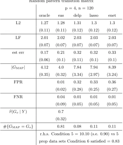
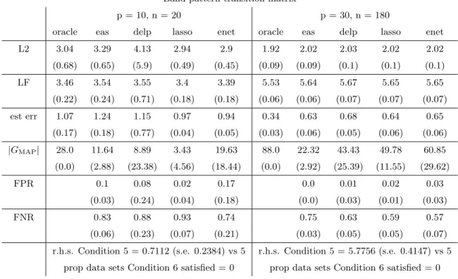
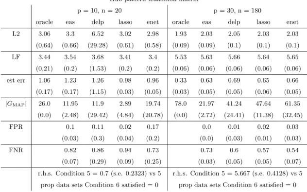
3.1 See Section 3.4.1 for definitions of each performance metric, except for the last two which are described in Section 3.4.2. All metrics are quantities averaged over 100 generated data sets, and standard errors are in parentheses. The ‘oracle’ column displays correspond-ing characteristics in the case that the oracle graph, Go, is known, and using the least squares estimate ofA0. Note that for Condition 5, 4(1 +c2) = 5. Recall that a new set of active componentsGo are generated for each data set, which gives the variability for |GMAP|
in the ‘oracle’ column. . . 59
3.2 See caption for Table 3.1. . . 61
3.3 See caption for Table 3.1. Recall that a new set of active components
Go are generated for each data set, which gives the variability for
|GMAP|in the ‘oracle’ column. . . 61
3.4 See caption for Table 3.1. . . 62
3.5 See caption for Table 3.1. Recall that a new set of active components
Go are generated for each data set, which gives the variability for
|GMAP|in the ‘oracle’ column. . . 62
3.6 See caption for Table 3.1. . . 63
4.1 Misclassification response function. . . 126
4.2 Displayed are the means and standard deviations of the (indepen-dent) normal priors placed on the 81 model parameters. Standard deviations are in parentheses, and these priors assume that the data have been centered. The parametersc1, . . . , c8are the control points
used to estimate the cubic spline for the state 1 to state 2 transition
(for baseline and age), as discussed at the end of Section 4.2.3. . . 132
4.3 Posterior mean estimates of the dementia diagnosis response pa-rameters. The components are probabilities. Note that each row corresponds to only one parameter, but both columns have been filled in for ease of interpretability (rows must sum to one). The brackets represent 95 percent credible intervals (for the components
LIST OF FIGURES
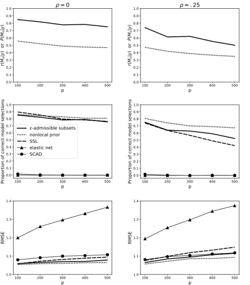
2.1 The average r(Mo|y), or average P(Mo|y) is displayed in the first row, the average proportion of correct model selections in the second row, and the average RMSE in the third. Averages are over 1000 synthetic data sets (for ρ = 0 and ρ = .25, respectively). For the GFI and Bayesian procedures the MAP subset is used as the estimator of the true model, and in the frequentist procedures the estimated model is considered to be the subset of covariates with nonzero coefficient estimates. The RMSE is computed on an
out-of-sample test set of 100 observations. . . 19
3.1 Directed graph of inclusion probabilities of components of the tran-sition matrix, A, for monthly closing stock price of 8 companies. First differences of the data are used. Each edge label represents the marginal generalized fiducial (or posterior-like) inclusion prob-ability of a particular component of A. That is, the proportion of graphs, G, (over all MCMC-sampled graphs) in which each com-ponent (i.e., edge) of A is active. Line widths are proportional to inclusion probabilities, and inclusion probabilities less than .05 are
omitted. . . 64
3.2 See description for Figure 3.1. . . 65
4.1 State space. Emitted response variables are displayed in brackets above the respective hidden state. A+ corresponds to high amyloid burden, and N+ corresponds to high neuro-degenerative burden.
States 1-4 are all non-demented. . . 116
4.3 Observed response data for PIB which is a measure of amyloid buildup from a PET scan, and (cortical) Thickness which is as-sociated with neuro-degeneration. Note that the response densities for PIB correspond to the data transformation, log(PIB−1). The component density estimates correspond to the posterior mean esti-mates from Section 4.5. The blue dashed lines represent the normal
mixture density estimates. . . 117
4.2 Observed response data for MMSE test scores associated with the six non-death states in the state space. The component density estimates here correspond to the posterior mean estimates from Section 4.5. The blue dashed line represents the normal mixture
density estimate. . . 117
4.4 Annualized natural logarithm of Minnesota overall population death rates. Solid line corresponds to female, and dashed line corresponds
4.5 Intercept coefficient estimates for a traditional study in which all subjects are enrolled at a common baseline time. ‘Bayes’ corre-sponds to the Bayesian posterior mean estimates, and ‘MLE (msm)’ corresponds to maximum likelihood estimates computed from the ‘msm’ function. Green dashed lines represent the true values. Cov-erage is the proportion of .95 probability credible intervals (con-fidence intervals for the MLE) which contain the true parameter
value. . . 128
4.6 Intercept coefficient estimates for a delayed enrollment study. ‘Bayes’ corresponds to the Bayesian posterior mean estimates, ‘MLE’ corresponds to the MLE obtained via optimizing the like-lihood function from Section 4.2.4 using the ‘optim’ function in R, and ‘MLE (msm)’ corresponds to maximum likelihood estimates computed from the ‘msm’ function. Green dashed lines represent the true values. Coverage is the proportion of .95 probability cred-ible intervals (confidence intervals for the MLE) which contain the
true parameter value. . . 129
4.7 Intercept and death rate bias coefficient estimates for the synthetic MCSA data, see (4.5) and (4.12). Note that the covariates in the data are centered. Presented are box plots of posterior means of the labeled parameters, from 50 synthetic MCSA data sets. Green dashed lines represent the true values. Coverage is the proportion of .95 probability credible intervals which contain the true parameter
value. . . 134
4.8 Evolution of transition probabilities. The curves represent the prob-ability of transitioning to the respective state for each given age, computed using the posterior mean estimates of the HMM parame-ters. The probabilities are conditional on not transitioning to state 7 (Dead), and correspond to an individual in state 1 (A−N−) at the baseline age of 50. The label ‘apoe4 negative’ corresponds to an individual with no APOE-ε4 alleles, and ‘apoe4 positive’ cor-responds to an individual with at least one APOE-ε4 allele. The curve labeled ‘Alzheimer’s’ depicts the probability of making the
transition from state 4 (A+N+) to state 6 (A+Dem), given not dead. . . 135
4.9 Posterior mean estimate of the death rate bias (4.12). Values are interpreted as the proportion of the population death rate that is experienced by subjects in the MCSA, for each integer year a subject is enrolled in the study. For example, subjects just enrolled in the study experience a death rate which is 31 percent of the population
4.10 Posterior mean estimates of thereciprocal transition rate compo-nents of Q at age 60. The numerical values can be interpreted as the estimated mean times (in years) to transition, conditional on age. These plots correspond to an individual with a college degree. Recall that transitions to dead from states 1-4 are constrained to
be equal, and so for ease of presentation only one transition arrow is shown. . 137
4.11 Posterior mean estimates of thereciprocal transition rate
compo-nents of Q at age 80. . . 138
5.1 A sample of realizations from the sampling distribution of the poste-rior density of the mean,θ, for Gaussian data with known variance and normal prior on θ. The green shaded region (Ac) is an ε-ball
around the true parameter value of θ. . . 143
5.2 The leftmost panel is a plot of the sampling probability, p, as a function ofε, as given by equation (5.3), forα=.5. The center and rightmost panels are randomly observed realizations of the posterior density of θ, with a .3-ball around θ0 represented by the shaded
green regions. In all panels, the true parameter value is set at θ0= 1. . . 146
5.3 The leftmost panel is a plot of the estimated sampling probability, b
pk, as a function of ε, as given by equation (5.4), for α =.5. The center and rightmost panels are randomly observed realizations of the posterior density of Ψ, with a 6-ball around ψ0 represented by
the shaded green regions. In all panels, the true parameter value is
set at ψ0 = 10. . . 148
5.4 Each panel is a plot of the estimated sampling probability ofp, as a function ofε, using the posterior density equation (5.5), and setting
α=.5. The true parameter value isψ0 = 10. . . 150
5.5 Each panel is a plot of the estimated sampling probability ofp, as a function ofε, using the posterior density equation (5.5), and setting
α=.05. The true parameter value isψ0 = 10. . . 150
5.6 Each panel exhibits randomly observed realizations of the posterior density of ψ, equation (5.5), with a 4-ball around ψ0 = 10
repre-sented by the shaded green regions. . . 151
5.7 Contour plots ofεas a function ofα andpfor three different values of n when θ0 = 1 and σ2 = 1. The value of ε for α = 0.5 and
p= 0.95 is marked with an X. . . 152
5.8 Gaussian model. εas a function ofnwhereα andpare fixed at 0.5
and 0.95, respectively. The true parameter isθ0 = 1. . . 152
5.9 Coefficient of variation. εas a function ofnwhereαandpare fixed
CHAPTER 1
Introduction
This dissertation is comprised predominantly of two topics of research. One involves exten-sive theoretical work on nonpenalized model selection problems encompassing both the high-dimensional linear regression and vector autoregression setting. The second is an application of a hidden Markov model (HMM) to the study of aging and the progression of dementia. Significant contributions of these projects are the implementation of alternative frameworks for statistical in-ference, namely, generalized fiducial inference (GFI) and Bayesian inference. A major theme of my research is to develop methods of statistical inference from epistemic perspectives which more naturally facilitate the interpretation of uncertainty quantification from data based on degrees of believe.
The nonpenalized model selection methodology and theory are presented in Chapters 2 and 3, the Bayesian HMM application is given in Chapter 4, and an additional chapter, Chapter 5, presents an exposition of an important theorem introduced recently in the literature which broadly impacts the foundations of statistical inference. Note that Chapter 3 is research which extends from the foundations built in Chapter 2. Nonetheless, each chapter in this dissertation represents completely developed and standalone research ideas. Each of these research topics are briefly introduced the remaining subsections.
1.1 Nonpenalized model selection via generalized fiducial inference
redundant information. Such subsets are common in situations with collinear covariates, and if it happens that the “true” data generating covariates are collinear, then only a strict subset of the covariates are needed to predict/explain the observed response data. We argue that in finite sample settings, focusing only on these nonredundant subsets is an avenue in which one can begin to relax assumptions of sparsity. Nevertheless, we prove mathematically that under a standard sparsity assumption, our variable selection procedure will assign probability 1 to the true model with probability converging to 1 as both the number of data observations, n, and covariates,p, are taken to infinity. Furthermore,p can be allowed to grow almost exponentially in n.
In extending the variable selection methodology from the linear regression setting to the multi-variate vector autoregressive (VAR) setting, we demonstrate an analogous asymptotic consistency result assuming the data are generated from a VAR(1) model (VAR model of order 1). Model selec-tion in this setting is best described as graph selecselec-tion (determining the active/inactive components of the transition matrix) because all variables (i.e., components of the VAR(1) model) are a part of the observed data, and thus cannot be omitted in the way covariates in a linear regression can. Theoretical investigations into high-dimensional VAR models are a very unexplored topic within the Bayesian, and of course GFI, literature. However, we are able to prove pairwise and strong
graphical selection consistency of the true graph, and demonstrate the effectiveness of our approach on high-dimensional synthetic data as well as real data.
1.2 A Bayesian approach to multi-state HMM: application to dementia progression
This research was entirely motivated by the Mayo Clinic Study of Aging (MCSA) and how the resulting data can be used to draw inference on the role of aging in the development of dementia. The goal was to create a model of progression to dementia which can accommodate: (1) a wide variation in age (the dominant variable under consideration), (2) significant fluctuation in the time between subject visits, (3) different amount of information available for each subject (e.g., missing visits and/or clinical data), and (4) subject specific covariates.
progression for studies like the MCSA. First, we provide an approach for correcting a common bias in delayed enrollment studies which has been overlooked in the literature. Second, we introduce a methodological framework for estimating the strength and persistence of a separate death rate biasspecific to death rates, which could be present in any study relying on enrollment of subjects. Our final methodological innovation is a Bayesian approach to estimating the biomarker regions most associated with high/low burden states in a manner that does not require the specification of cut-points. Hard cut-points for discretizing continuous measurements of biological processes are practically and philosophically problematic, and have to be chosen more or less arbitrarily.
Note, the termdelayed enrollment, here, is used to describe a study with a given baseline (age 50 in the case of the MCSA) such that some or all subjects are not observed at baseline. We demonstrate empirically that the effects of this bias cannot be ignored, and existing software is not equipped to handle this feature. Moreover, we illustrate a general and effective framework for fitting a continuous-time, discrete-state HMM within the Bayesian paradigm, and the infinitesimal generator matrix of the underlying Markov process is allowed to be truly time-inhomogeneous (as a function of an individual’s age).
1.3 An exposition of the false confidence theorem
CHAPTER 2
Nonpenalized variable selection in high-dimensional linear model settings via
generalized fiducial inference
2.1 Introduction
A strategy for developing variable selection procedures with desirable consistency properties entails exploiting some distinguishing property of the theoretical true data generating model. For example, standard penalized methods of variable selection within a linear model framework such as LASSO of Tibshirani (1996), SCAD of Fan and Li (2001), and the Dantzig Selector of Candes and Tao (2007) rely on the magnitude of the coefficients in the true data generating model being relatively larger than those of the other coefficients. Johnson and Rossell (2012) use this property to construct nonlocal prior densities over all subsets of covariates. The defining property of their nonlocal density is that it takes the value of zero for subsets containing a covariate with a zero-valued coefficient.
We propose a more desirable way for eliminating redundancies from the sample space of candi-date subsets which does not explicitly rely on coefficient magnitudes. That is, any candicandi-date true model should be non-redundant in the sense that it contains the minimal amount of information necessary for explaining and/or predicting the observed data. One such criterion to exploit this non-redundancy property is that the only subsets with nonzero posterior probability should be those which cannot be predicted to some chosen precision by a subset of fewer covariates. Such a criterion requires constructing a probability distribution on the space of candidate models, which is consis-tent with a Bayesian or fiducial variable selection paradigm. The literature on high-dimensional linear models is vast, but we hope to contribute to it by using this setting to build a foundation for a fresh perspective on variable selection.
the credible set approach of Bondell and Reich (2012), and Narisetty and He (2014) who propose a method based on shrinking and diffusing coefficient priors in which the variance of the priors are sample size dependent. Lai et al. (2015) layout framework for penalized estimation within a GFI approach.
Ghosh and Ghattas (2015) provide insights into complications in Bayesian variable selection. Namely, the size of the sample space (2p) is often too large to compute all model probabilities, and even typically larger than can reasonably be sampled by Markov chain Monte Carlo (MCMC) methods. Thus, the nonlocal prior approach of Johnson and Rossell (2012) can achieve asymptotic consistency (where other approaches can only achieve asymptotic pairwise consistency) because it is able to effectively eliminate a large enough portion of the 2p subsets from the sample space. To illustrate this point, consider the following simple example. Let
Y ∼Nn
β1·x(1)+· · ·+βp·x(p), σ2In
, (2.1)
where βj ∈ R and x(j) ∈ Rn for j ∈ {1, . . . , p}, and σ > 0. Further, suppose that the
true but unknown values of (β1, β2, β3, . . . , βp)0 are (b1, b2,0, . . . ,0)0. Within the nonlocal prior
framework, the only subsets with non-negligible posterior probability are contained in the set
{x(1)},{x(2)},{x(1), x(2)} .
When viewed as a prior density on the coefficients, nonlocal priors assign zero prior density to the true parameter value when the true parameter value is zero. From a Bayesian perspective this is philosophically problematic, but very insightful for consistency of model selection. The insight lends itself to the question: What other properties might the true model have which can be exploited to develop a statistical procedure with the ability to effectively eliminate subsets from the sample space?
To further illustrate the intuition behind our proposal, consider an example where x(2) is highly collinear with all of x(3), . . . , x(p) but is notcorrelated with x(1), and where the true values of (β1, β2, β3, . . . , βp)0are (b1, b2, b3, . . . , bp)0withbj 6= 0 for allj∈ {1, . . . , p}. In this case, assuming strong enough collinearity,∃c∈R withc·x(2) ≈b2·x(2)+· · ·+bp·x(p), i.e.,
b1·x(1)+· · ·+bp·x(p)
− b1·x(1)+c·x(2)
< ε
where ε > 0 is some desired precision. Thus, for much of the parameter space the subset {x(1), . . . , x(p)} is not ε-admissible, but would be assigned nonzero posterior probability in the
nonlocal prior framework.
We construct a posterior-like probability distribution over all subsets, which assigns negligible probability to elements that are not ε-admissible. In constructing the posterior-like probability distribution we adopt a generalized fiducial inference (GFI) approach because it has similar to an objective Bayes interpretation with data driven priors, gives a systematic method of constructing a distribution function given a data generating equation such as a linear model, and it does not suffer from the issue of arbitrary normalizing constants which arise in many objective Bayesian priors (Berger and Pericchi (2001)). In this manuscript we will provide a gentle introduction to GFI. A fuller account of GFI is given in the recent review paper Hannig et al. (2016).
An advantage of both our approach and the nonlocal prior approach of Johnson and Rossell (2012) is that in addition to providing theoretical guarantees, our statistical procedures yield es-timates of the posterior distribution over subsets of covariates. This is in contrast to frequentist penalization based methods or Bayesian procedures fully dedicated to maximum a posteriori prob-ability (MAP) estimation. Such methods do not yield the posterior probprob-ability of a chosen model (i.e., the relative probability, given the observed data, of a given model against competing models). Furthermore, Ghosh and Ghattas (2015) argue that joint summaries of subsets of covariates are more robust to collinearity.
almost exponentially in n. The reason being that the true model yields a stronger signal since it no longer has to compete within an overly redundant sample space.
The paper is organized as follows. Section 2.2 serves to introduce the general methodology and computational algorithm for carrying out our variable selection procedure based on a recent algorithm for explicit L0 minimization (Bertsimas et al. (2016)), which is fast enough to be used
on real data. The conditions needed for the main results, and the main results are presented and discussed in Section 2.3. Proofs are organized in the appendix. We demonstrate the empirical per-formance of our procedure and compare it to other Bayesian and frequentist methods in simulation setups on synthetic data in Section 2.4. Computer code implementing our procedure is provided
athttps://jonathanpw.github.io/software.html.
2.2 Methodology
As described in the previous section, our idea behind exploiting a non-redundancy property of the true data generating model relies on constructing a probability distribution concentrated on what we denote asε-admissiblesubsets. This object is defined precisely in Definition 2.1, but first an aside on the notation used throughout the paper.
The function|·|denotes the absolute value function if its argument is scalar-valued, and denotes the cardinality function if its argument is set-valued. The normsk · k2 andk · k0 refer, respectfully, to the usualL2 andL0 norms defined on finite-dimensional Euclidean spaces. Lastly,k · kF denotes the matrix Frobenius norm.
Let Y be an n-dimensional random vector, X an n×p matrix with columns scaled to have unit norm, and β0 a fixed p-dimensional vector with nonzero (or active) components indexed by the subsetMo ⊂ {1, . . . , p}, with
Y ∼Nn
XMoβ 0
Mo,(σ 0
Mo) 2I
n
. (2.2)
The design matrix denoted by XMo is defined as the matrix composed of only those columns of
X corresponding to the index set Mo. The subscript ‘o’ refers to the interpretation of Mo as corresponding to the ‘oracle’ subset of covariates. Moreover, βM0
o denotes the true values of the
oracle coefficients, while βMo is understood as a random vector whose uncertainty resides in not
column space ofXM on the true coefficientsβ0Mo, that is,β
0
M = (XM0 XM)−1XM0 XMoβ
0
Mo =Ey(βbM).
The subscript on Ey(·) is used to denote the expectation taken with respect to the sampling distribution of the data Y. Lastly, σ0Mo > 0 denotes the true unknown error standard deviation, whileσMo is a random variable whose distribution expresses the uncertainty from not knowingσ
0
Mo,
under the oracle model.
The objective is to construct a statistical procedure which can be shown, asymptotically and demonstrated empirically, to be able to identifyMoas the index set of the oracle model within the sample space of all 2p candidate subsets M ⊂ {1, . . . , p}. For each index set, M, in the sample space the conditional sampling distribution of the data is assumed as
Y|βM, σM2 ∼Nn
XMβM, σM2 In
. (2.3)
The centerpiece of our methodology is then the following definition.
Definition 2.1. Assume fixedε >0. A givenβM coupled within some index subsetM ⊂ {1, . . . , p} is said to beε-admissibleif and only if h(βM) = 1, where
h(βM) := I n1
2kX
0(X
MβM −Xbmin)k22≥ε
o
, (2.4)
and bmin solves min
b∈Rp 1 2kX
0(X
MβM −Xb)k22 subject to kbk0 ≤ |M| −1.
Observe that this definition is consistent with the heuristic description of ε-admissiblesubsets given in the previous section. In particular, if the subset of covariates indexed by M is linearly dependent or if one of the components ofβM is zero, thenh(βM) = 0. The subtlety in this definition is assuming an appropriately chosenεwhich is able to strike an optimal balance for distinguishing signal from noise. Intuitively, ε = ε(n, p, M), i.e., is a function of the amount of information available given byn, the difficulty of the problem represented byp, and information about a given
M being considered such as |M|. For instance, if |M|> n then h(βM) = 0 because XM cannot have full rank. In this case any ε >0 will work, but the choice ofε matters a lot if |M| ≤n. The choice of εis a major focus of Section 2.3 where the main results of the paper are presented, and from where we suggest the following default choice:
ε= ΛMbσ2M n0.51
9 +|M|
log(pπ)1.1
9 −po
+
, (2.5)
where ΛM := kHMXk2F and bσ
2
M := RSSM/(n− |M|) with RSSM := y
0(I
n−HM)y and HM :=
po represents prior belief about|Mo|, the number of covariates in the true modelMo. In practice, a value of po can be directly specified or selected by cross-validation. A built-in cross-validation procedure is included in the accompanying software to this paper. Details are provided with the simulation study in Section 2.4.
Within the h function in Definition 2.1 the quantity 12kX0(XMβM −Xbmin)k22 represents the
difference in prediction for a subset M against all subsets with fewer covariates. This measure of distance has been adapted from Candes and Tao (2007), but they deal with the errorkX0(y−Xb)k∞
overb∈Rp. This is very different from usingX
MβM in place of y because the former results in a noiseless measure of distance. To illustrate, observe that
Ey kX0(Y −Xb)k22
=kX0(XMoβMo −Xb)k
2
2+σM2o ·p.
There are various reasons for using the quantity X0(XMβM −Xb) from the Dantzig selector (Candes and Tao (2007)) versus simply the difference in predictions (XMβM−Xb) as in the LASSO (Tibshirani (1996)). One reason is that X0(XMβM −Xb) accounts for difference in predictions as well as correlations with the explanatory data, as discussed in Berk (2008). If the difference in predictions is small but is highly correlated with the design matrix, then it is likely that the smaller subset of covariates is unable to account for the effect of one or more of the covariates inM. Thus, using X0(XMβM −Xb) instead of just the difference in predictions is a method of controlling for potential omitted variable effects which could incorrectly find a close fitting subset toM. Another advantage ofX0(XMβM−Xb) is that it is invariant under orthogonal transformations of the design matrix, as pointed out in Candes and Tao (2007).
To illustrate as in Hannig et al. (2016), suppose that some dataY =G(U, θ) for some determin-istic data generating equation G(·,·), some parameters θ, and some random component U whose distribution is independent ofθ and is completely known. The generalized fiducial distribution of
θ is then given by
r(θ|y) = R f(y, θ)J(y, θ)
Θf(y, θ0)J(y, θ0)dθ0 ,
wheref is the likelihood function and
J(y, θ) =D
d
dθG(u, θ)
u=G−1(y,θ)
with D(A) = (detA0A)12. The component J(y, θ) is termed the J acobian because it results from
inverting the data generating equation on the data. We are committing a slight abuse of notation as r(θ|y) is not a conditional density in the usual sense. Instead, we are using this notation to stress that the generalized fiducial distribution is a function of the observed datay.
To make matters concrete in the linear model setting of (2.3), the parameters areθ= (βM, σM), the data generating equation is specified asG U,(βM, σM)
=XMβM+σMU whereU ∼Nn(0, In), and the Jacobian term reduces to J y,(βM, σM)
=σ−M1|det(XM0 XM)|
1
2RSS
1 2
M. Thus,
r (βM, σM)|y
∝σM−ne−
ky−XM βMk22
2σ2
M σ−1
M |det(X
0
MXM)|
1
2RSS
1 2
M ·h(βM),
where the factor ofh(βM) appears in the likelihood from only considering ε-admissiblesubsets of the parameter space. Accordingly, as is done with a Bayesian posterior density and in Section 3 of Hannig et al. (2016), define the GFI probability of a given subset M to be proportional to the normalizing constant of r (βM, σM)|y
. That is,
r(M|y) :=
R
f y,(βM, σM)
J y,(βM, σM)
h(βM)d(σM, βM) p
P j=1
P
|M|=j R
f y,(βM, σM)
J y,(βM, σM)
h(βM)d(σM, βM)
∝
Z
RpM Z ∞
0
h(βM)
|det(XM0 XM)|
1 2RSS
1 2
M
σnM+1e
(y−XM βM)0(y−XM βM) 2σ2
M
dσM dβM,
which simplifies to
r(M|y)∝π|M2|Γ
n− |M| 2
RSS−(
n−|M|−1 2 )
M E(h(βM)), (2.6)
where the expectation is taken with respect to the location-scale multivariate T distribution,
tn−|M|
b
βM,
RSSM
n− |M|(X
0
MXM)−1
with βbM := (XM0 XM)−1XM0 y. Notice that the quantity E(h(βM)) is a function of the observed datay.
Observe that (2.6) expresses the relative likelihood of the subsetM over all 2ppossible subsets. The expression can be described as a product of two terms, the first being comprised of information from the sampling distribution of the data and largely driven by the residual sum of squares, RSSM, and the second having to do with the ε-admissibility of βM, in the form of E(h(βM)). Thus, the support ofr(M|y) in (2.6) is dominated by the ε-admissiblesubsets, as desired.
Section 2.3 provides the conditions and supporting lemmas and theorems needed to show that
r(Mo|Y) → 1 in probability as n, p → ∞. First however, a few remarks are provided about computing r(M|y) on actual data.
2.2.1
Remarks on computation
With a probability distribution now defined overε-admissiblesubsets, it must be demonstrated thatr(M|y) in (2.6) can be efficiently computed. There are two main computational issues to deal with. The first is to evaluate h(βM) for a given βM, and the second is to sample subsets M via pseudo-marginal based MCMC. The computational complexity and the need for pseudo-marginal based MCMC arises because neitherh(βM) nor E(h(βM)) have a closed form solution.
To evaluateh(βM) for a givenβM we adapt an explicitL0 minimization algorithm introduced
in Bertsimas et al. (2016). The authors state that their algorithm borrows ideas from projected gradient descent and methods in first-order convex optimization, and solves problems of the form minb∈Rpg(b) subject tokbk0 ≤κ, where g(b) ≥0 is convex and has Lipschitz continuous gradient:
k∇g(b)− ∇g(eb)k2 ≤lkb−ebk2. The algorithm is not guaranteed to find a global optimum (unless formal optimality tests are run, which can take a long time), but Bertsimas et al. (2016) provide provable guarantees that the algorithm will converge to a first-order stationary point, which is defined as a vector ˜b ∈ Rp with k˜bk
0 ≤ κ which satisfies ˜b = ˜b− 1l∇g(˜b). Paraphrasing from
Bertsimas et al. (2016), their algorithm detects the active set after a few iterations, and then takes additional time to estimate the coefficient values to a high accuracy level. In our application of their algorithm we are not first-most interested in finding a global optimum. To evaluate h(βM), we need only determine if minb∈Rp1
2kX
0(X
quickly via our implementation of the L0 minimization algorithm. To illustrate how consider the
following specifics of our implementation. The precise details regarding the algorithm can be found accompanying our software documentation at https://jonathanpw.github.io/software.html.
First, to estimateE(h(βM)) we use a sample mean of sample vectors drawn from the location-scale multivariate T distribution in (2.7). This multivariate T distribution is centered at the least squares estimator, βbM, and multivariate theory suggests that βbM will on average be close to the coefficientsβ0
M. By warm starting theL0minimization algorithm atβbM with the smallest coefficient removed, subsets corresponding toβM0 with at least one zero coefficient typically yield h(βM) = 0 within a few steps of the algorithm.
Second, as per the definition ofh(·) in (2.4) the objective function is minimized over allb∈Rp withkbk0≤ |M| −1. Hence, theκrequired for theL0 minimization algorithm from Bertsimas et al.
(2016) is naturally chosen for us as κ = |M| −1. Knowing how to choose κ greatly reduces the
L0 optimization problem. Moreover, our implementation is further simplified by the fact that the
closest prediction to XMβM for a givenM is guaranteed to have|M| −1 covariates. Accordingly, the objective function in h(βM) need notbe minimized over all b∈ Rp with kbk0 ≤ |M| −1, but
can be minimized over allb∈Rp withkbk
0 =|M| −1.
The second computational issue is to sample subsetsM via pseudo-marginal based MCMC. We do this by using the Grouped Independence Metropolis Hastings (GIMH) algorithm from Andrieu and Roberts (2009), but originally introduced in Beaumont (2003). The reason standard MCMC techniques do not apply is that there is no obvious closed form expression for the probability mass function (2.6) because of the expectation,E(h(βM)), in the expression. As described in Andrieu and Roberts (2009) such situations warrant introducing a latent variable to yield analytical expressions or easier implementation.
from slower mixing than if we were able to integrate the βM out of the mass function r(M|y) in (2.6), i.e., analytically evaluate E(h(βM)). However, this is not possible given the h function in (2.4). Additionally, the mixing associated with pseudo-marginal approaches is known to be poor when the number of importance samples (N, the sample size of B) is small. These practical bottlenecks outline avenues for future research. Nonetheless, we demonstrate in Section 2.4 that our computational strategies are efficient enough to be implemented on actual data, in comparison to other common penalized likelihood and Bayesian approaches.
2.3 Theoretical results
The main objective of this section is to show under what conditions, asymptotically, r(Mo|Y) in (2.6) will converge to 1, particularly if p >> n. The ε-admissible subsets approach is able to achieve such a strong consistency result because the resulting sample space is effectively reduced to only those subsets with no redundancies. The essence of the mathematical result is that the space ofε-admissiblesets is small enough that the true model can be detected. This addresses the issue raised in Ghosh and Ghattas (2015) that high-dimensional settings often lead to arbitrarily small probabilities for all models (including the true model) simply because there are too many models to consider.
2.3.1
Discussion of the conditions
The first two conditions, Condition 1 and Condition 2, are to ensure that the true model,
Mo, is identifiable. Observe from (2.4) that ε is used to control the sensitivity and specificity for identifyingε-admissiblesubsets. In particular, if εis too large, then h(βMo) will incorrectly be set
to zero implying thatβMo is notε-admissible. Condition 1 specifies how large εcan be whilst the
true model remains identifiable. This condition turns out to be critically important in actual data applications because computingh(βMo) is closely related to the comparison in equation (2.8).
Condition 1. For large n andp,
1 18kX
0(X
Moβ 0
Mo−Xbmin)k 2
2≥ε (2.8)
where bmin solves min
b∈Rp
1 2kX
0(X
Moβ
0
Mo −Xb)k
2
Condition 2 is born from Lemma 3 which is an important necessary result for the main result of this paper, Theorem 3. The term log(n)γ represents the sparsity assumption for the true model, i.e., the number of covariates in the true model must not exceed log(n)γ for some fixed scalarγ >0. The γ parameter indicates that the asymptotic results remain true if the true model grows faster than log(n), but not faster than some power of log(n). In finite-sample applications, γ has no consequence and can be ignored.
The constant α ∈ (0,1) reflects the only explicit restriction needed on the sample space of 2p subsets to show thatr(Mo|Y) → 1 in probability for large n and p, Theorem 3. The residual sum of squares term inr(M|Y) in (2.6) cannot be controlled (as a ratio tor(Mo|Y)) for arbitrary subsetsM with|M|=O(n) because the column span ofXM includesy ∈Rnwhen rank(XM) =n. To eliminate such subsets from the sample space, Condition 2 requires that only subsets of size |M| ≤ nα can be given nonzero probability. However, recall from Definition 2.1 thath(βM) = 0 if |M|> n because in this case the columns ofXM must be linearly dependent. Accordingly, all subsets M with|M|> n are given zero probability, by definition. Evidenced by this fact, the only explicit restriction placed on the sample space is that subsets M with |M| ∈(nα, n) are excluded. In sparse settings it is assumed that |Mo|<< n anyway, so neglecting such subsets is reasonable. Convergence to the true model Mo will be quicker for smaller α because there are less models to consider, but too small of anα will exclude Mo from the sample space.
In Condition 2, and for the remainder of this section assume that γ > 0, say γ = 1, and
α∈(0,1), say α=.5, have been chosen and fixed at appropriate values.
Condition 2. The true model Mo satisfies |Mo| ≤log(n)γ, and
lim n→∞
p→∞
minn ∆M |Mo|log(p)
:M 6=Mo,|M| ≤ |Mo| o
=∞,
lim infn→∞ p→∞
n1−α
log(p) >2, and log(p)<
n− |Mo| −1 4 log(n)γ ,
for large nand p, where ∆M :=kXMoβ
0
Mo −HMXMoβ
0
Mok
2
2 as in Lai et al. (2015).
This is a slightly weaker version of condition (11) in Lai et al. (2015). They relate Condition 2 to the sparse Riesz condition (Zhang and Huang (2008)) which requires that the eigenvalues of XM0 XM/n are uniformly bounded away from 0 and ∞. Essentially, ∆M is a measure of how distinct the true model predictions XMoβ
0
XM for M 6=Mo and |M| ≤ |Mo|. Recall that HM := XM(XM0 XM)−1XM0 . In particular, if XM is orthogonal to XMo, then ∆M = kXMoβ
0
Mok
2
2 which will be much larger than the denominator, |Mo|log(p). The requirements of this condition are reasonable because ∆M grows very fast forM such thatMo 6⊆M.
Condition 2 is important for being able to identify the true model amongst other models M
with|M| ≤ |Mo|. The next two conditions address the requirements forM with|M|>|Mo|, which primarily rely on the fact that such subsets are notε-admissible.
Conditions 3 and 4 demonstrate how largeεneeds to be to achieve the consistency result of the main theorem. Condition 3 states that for subsets of covariates with redundancies, ε needs to be larger than the difference in projections of the true model prediction,XMoβ
0
Mo, ontoM and onto a
strict subset ofM. This condition facilitates the intuition that the variable selection procedure will not concentrate on subsets M with redundant covariates. If a given subset M is notε-admissible, then the difference in projections will be small so that the condition is easily achieved.
Condition 3. For any M with |M|>|Mo|, for large n or p, 9
2kX
0(H
M −HM(−1))XMoβ
0
Mok
2 2 < ε,
where HM(−1) is the projection matrix for M after omitting the covariate which minimizes kX0(HM −HM(−1))XMoβ
0
Mok
2 2.
In fact, if Mo ⊂ M with |Mo| < |M|, then HMXMoβ
0
Mo = HM(−1)XMoβ
0
Mo in which case
Condition 3 holds trivially.
Lastly, Condition 4 describes the rate at which ε needs to grow to achieve the consistency of the main result. The distinction between Condition 3 and Condition 4 is that the former provides a necessary lower bound for arguing that E(h(βM)) vanishes for M such that |M|> |Mo|, while the latter provides the rate at whichεmust grow to achieve the consistency result of Theorem 3.
Condition 4.
lim n→∞
p→∞
min
|M|≤nα
ε
18ΛMσb
2
M
+D1|Mo| −ϕ(M, n, p) log(n) =∞,
where
ϕ(M, n, p) := 4e2nα+ (D1+ (1 + 4e2) log(p))|M|+ log
|M| 1− 1
n−|M|
!
,
and D1 = 12log
6π
1−nαn+2
. Additionally, 9Λ ε
Mbσ
2
M
The terms which compete with ε arise in the proofs of Lemma 3 and Theorem 3. Recall that
b
σM2 := RSSM/(n− |M|), where RSSM is the classical residual sum of squares for model M, and that ΛM := kHMXk2F. The ΛM term arises from Lemmas 1 and 2. It is intimately related to the presence of collinearity amongst the covariates, and Condition 4 implies that ε must account for collinearity by controlling for ΛM. Observe that ifX is orthogonal, then ΛM =|M|.
2.3.2
Main result
The first two results are lemmas which are needed in the proofs of Theorems 1 and 2. Lemma 1 illustrates the rate at which βM concentrates around its mean, βbM, the least squares estimator, and Lemma 2 illustrates the rate at which βbM concentrates around its mean, Ey(βbM). Theorem 1 uses these two lemmas to bound the rate at which βM concentrates around Ey(βbM) for subsets
M with|M|>|Mo|. This yields an upper bound onE(h(βM)) with a probabilistic guarantee, and implies that E(h(βM)) vanishes for large n and p, for large non-ε-admissible subsets. The proofs are relegated to Appendix 2.7.
Lemma 1. For any fixed c1 ∈(0,1) assume |M| ≤c1n, and choose n and p such that 9Λ ε
Mbσ
2
M
<
n−|M|
2 . If
βM ∼tn−|M|
b
βM,
RSSM n− |M|(X
0
MXM)−1
,
where βbM = (XM0 XM)−1XM0 y, then
P
1 2kX
0
XM(βM −βbM)k22 ≥
ε
9
≤ 2 3
23|M|
b
σM √
ΛMe−
ε
18ΛMbσ
2
M
√
πε(1− 1
n−|M|) .
In the next lemma,Py is used to denote the probability measure associated with the sampling distribution of the dataY.
Lemma 2. Assume |M|< n, and Y|βM, σM2 ∼Nn
XMβM, σ2MIn
. Then the least squares
esti-mator βbM ∼N|M|
Ey(βbM), σM2 (XM0 XM)−1
, and
Py 1
2kX
0
XM βbM −Ey(βbM)
k22≥ ε 9
≤ 3|M|σM √
ΛM √
πε e
− ε
9σ2
MΛM.
Theorem 1. For any fixed c1 ∈ (0,1) suppose |Mo| < |M| ≤ c1n, choose n and p such that
ε
9ΛMbσ
2
M
< n−|2M|, and assume thatε satisfies Condition 3. Then
Py
E(h(βM))≤
2323|M|
b
σM √
ΛM √
πε(1− 1
n−|M|) e−
ε
18ΛMbσ
2
M
≥1− 3|M|σM √
ΛM √
επe
ε
9σ2
MΛM
.
The next result is a probabilistic guarantee the true model is ε-admissible given ε satisfies Condition 1. This result is a statement that Mo is identifiable.
Theorem 2. For any fixed c1 ∈ (0,1) suppose |Mo| ≤ c1n, choose n and p such that 9Λ ε
Moσb
2
Mo
<
n−|Mo|
2 , and assume thatε satisfies Condition 1. Then
Py E(h(βMo))≥1−
2323pM
obσMo
p ΛMo
√
πε(1− 1
n−pMo)e ε
18ΛMobσ
2
Mo
!
≥1−3pMoσMo
p ΛMo
√
επe
ε
9σ2
MoΛMo
.
The following result is the main result of the paper. It shows that the ratio of the generalized fiducial probability of the true model to the sum over that of all other subsets of covariates M
satisfying |M| ≤nα will converge to 1 in probability for largenandp. Note that the restriction to subsetsM with|M| ≤nαis a stronger restriction than|M| ≤c1n, which is sufficient for Theorems
1 and 2. The reason being that the main result is stronger than the results of these two theorems. In fact, Theorems 1 and 2 are non-asymptotic results that hold for each fixed modelM separately, while Theorem 3 is an asymptotic result which applies uniformly over all|M| ≤nα. Just like with a conditional distribution, r(M|Y) is obtained by replacing the observed data y with the random variableY (random with respect to the sampling distribution), in (2.6).
Theorem 3. Given Conditions 1-4, the true model Mo satisfies,
r(Mo|Y) Pnα
j=1
P
M:|M|=jr(M|Y) Py
−→1
as n→ ∞ or n, p→ ∞.
2.4 Simulation results
This section serves to demonstrate the empirical performance of our algorithm on synthetic data. It is comprised of essentially two simulation setups. The first setup, similar to that presented in Johnson and Rossell (2012), compares our procedure to the nonlocal prior approach, the spike and slab LASSO of Roˇckov´a and George (2018), the elastic net as implementated in the P ython
module scikit-learn (Pedregosa et al. (2011)), and to the SCAD as implementated in the R
packagencvreg(Breheny and Huang (2011)). The authors of the nonlocal prior and the spike and slab LASSO, respectively, have made available the R packages mombf and SSL for implementing their methods.
The second setup illustrates a critical difference between our ε-admissible subsets and the nonlocal prior approach. Namely, for highly collinear finite-sample settings in which the true model is not uniquely expressed, given the level of noise in the data (i.e., σM0 o), we demonstrate that our approach concentrates (in the sense of the MAP estimator) on subsets with fewer covariates without sacrificing prediction error. The intuition for why this should be the case was discussed in Section 2.1.
2.4.1
Simulation setup 1
Here we generate 2000 data vectorsyaccording to model (2.2) withMoconsisting of 8 covariates corresponding to βM0
o = (−1.5,−1,−.8,−.6, .6, .8,1,1.5)
0, and σ0
Mo = 1. The n×p design matrix
X is generated with rows from the Np(0,Σ) distribution, where the diagonal components Σii = 1 and the off-diagonal components Σij =ρ fori6=j. The first 1000 y correspond to an independent design withρ= 0, while the last 1000ycorrespond toρ=.25, as in the simulation setup of Johnson and Rossell (2012). Note that 2000 design matricesX are generated, and oney is generated from each design. The sample size nis set atn= 100, andp= 100,200,300,400,500 are all considered. We implement our algorithm on each of the 2000 synthetic data sets for 15000 MCMC steps with the first 5000 discarded. Squared coefficient estimates from elastic net (using scikit-learn) added by n−2 serve as MCMC covariate proposal weights. The default εin (2.5) is used, and we
100 200 300 400 500 p
0.0 0.1 0.2 0.3 0.4 0.5 0.6 0.7 0.8 0.9 1.0
r(Mo
|y)
o
r
P(
Mo
|y)
= 0
100 200 300 400 500
p 0.0
0.1 0.2 0.3 0.4 0.5 0.6 0.7 0.8 0.9 1.0
r(Mo
|y)
o
r
P(
Mo
|y)
= . 25
100 200 300 400 500
p 0.0
0.1 0.2 0.3 0.4 0.5 0.6 0.7 0.8 0.9 1.0
Proportion of correct model selections
-admissible subsets nonlocal prior SSL elastic net SCAD
100 200 300 400 500
p 0.0
0.1 0.2 0.3 0.4 0.5 0.6 0.7 0.8 0.9 1.0
Proportion of correct model selections
100 200 300 400 500
p 1.0
1.1 1.2 1.3 1.4
RMSE
100 200 300 400 500
p 1.0
1.1 1.2 1.3 1.4
RMSE
Figure 2.1: The averager(Mo|y), or averageP(Mo|y) is displayed in the first row, the average proportion
of correct model selections in the second row, and the average RMSE in the third. Averages are over 1000 synthetic data sets (for ρ= 0 andρ=.25, respectively). For the GFI and Bayesian procedures the MAP subset is used as the estimator of the true model, and in the frequentist procedures the estimated model is considered to be the subset of covariates with nonzero coefficient estimates. The RMSE is computed on an out-of-sample test set of 100 observations.
the Bayesian information criterion (BIC) on the held-out test set, and the computed BIC values are averaged over the 10 test sets, for each po ∈ {1,2, . . . ,10}. The po corresponding to the minimum average test set BIC is then selected.
Finally, for our implementation of the algorithm post-selection ofpo, the number of importance samples for estimatingE(h(βM)) within each step of the algorithm is set atN = 100 which, through empirical experimentation, seems to be enough. All competing variable selection procedures are implemented using existing software at default specifications. The one exception is that the nonlocal prior procedure is set to run for 5000 steps, as is the case in the simulation setup of Johnson and Rossell (2012). The nonlocal prior procedure/software did not scale well for increased p, and required over a weeks worth of parallel computations on a computing cluster to obtain the results for the first simulation setup. The tuning parameters for all methods are chosen with the default cross-validation procedures provided with the software. Lastly, as in the simulation section for Roˇckov´a and George (2018) theirλ1 is set at 1 (with a grid of 20λ0 values ending at 50), and their
adaptive (best performing) procedure is used withθ∼Beta(1, p).
Figure 2.1 shows results of the first simulation setup. The first row of plots displays the average generalized fiducial probability of the true model (i.e., average r(Mo|y)), or the average posterior probability of the true model for the Bayesian nonlocal procedure (i.e., averageP(Mo|y)), over the 1000 synthetic data sets (for ρ = 0 and ρ = .25, respectively). Conditional on the data, these plots address the consistency of the procedures with respect to the uncertainty from not knowing
Mo. This generalized fiducial or Bayesian-like consistency is that which is dealt with in Theorem 3. Note that frequentist and MAP estimators do not yield posterior probability estimates, and thus cannot be compared to in the first row of plots.
MAP estimated model is used to compute the RMSE for the GFI and Bayesian procedures. For all procedures, the RMSE is computed on an out-of-sample test set of 100 observations.
Note that the criterions used in the first two rows of Figure 2.1 are very strict. They only reflect instances when the procedures are exactly correct, and count the procedure as incorrect if it is missing even one covariate from the true model or includes even one spurious covariate. Often the elastic net and SCAD are able to identify all of the true covariates but estimate extra coefficients to be nonzero. This results in poor identification of the true subset, and worse out-of-sample prediction error. The remaining procedures (including our ε-admissible subsets method) struggle to identify the two covariates with smallest coefficient magnitudes, but typically do not introduce more than one or two false positives.
Our ε-admissiblesubsets procedure evidently performs the best at assigning highest posterior probability to the true model. And even in comparison to the frequentist-oriented metrics, pro-portion of correct model selections and out-of-sample RMSE, our ε-admissible subsets procedure performs more or less on par with the best performing methods considered.
In collinear design settings (i.e., ρ > 0) it may be the case that a strict subset of the true data generating model is identified as the ‘true’ model within the ε-admissible framework. This is meaningful because it manifests the fact that the true model may not be minimal (i.e., con-tains redundant predictors) in collinear, finite-sample settings. Furthermore, it explains the larger difference in proportion of true model selections between the ε-admissibleand nonlocal prior per-formances in the ρ =.25 case (versus the ρ= 0 case), which is accompanied by only a very small change in the difference between RMSE performance. An interpretation is that for highly correlated covariates theε-admissible subsets method may not recover the correct set of predictors (or does so less frequently), but instead it recovers a smaller set that results in almost the same predictions (as can be seen from the RMSE in Figure 2.1). This phenomenon is illustrated in a more extreme case of collinearity in the next simulation setup.
2.4.2
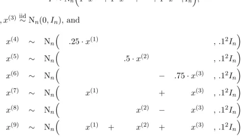
Simulation setup 2
following setup in which the true data generating model lacks uniqueness for the small sample size
n= 30:
Y ∼Nn
1·x(1)+ 1·x(2)+· · ·+ 1·x(9), In
, (2.9)
wherex(1), x(2), x(3) iid∼Nn(0, In), and
x(4) ∼ Nn
.25·x(1) ,.12In
x(5) ∼ Nn
.5·x(2) ,.12In
x(6) ∼ Nn
− .75·x(3) ,.12In
x(7) ∼ Nn
x(1) + x(3) ,.12In
x(8) ∼ Nn
x(2) − x(3) ,.12In
x(9) ∼ Nn
x(1) + x(2) + x(3) ,.12In
With standard deviations of .1 and a model error standard deviation of 1, covariates x(4), . . . , x(9)
can all be approximately expressed as a linear combination of x(1), x(2), x(3). Accordingly, with a small increase in error variance, model (2.9) can be re-expressed using various combinations of the 9 predictors. However, observe that a subset with 4 or more predictors predominantly contains redundant information.
Recall from Section 2.1 that the nonlocal prior approach of Johnson and Rossell (2012) is designed to assign negligible probabilities to subsets containing predictor(s) with coefficients of zero. So, in theory, the full subset{x(1), . . . , x(9)}will remain the best candidate for the true model within the nonlocal prior framework. In fact, this is demonstrated to be the case in Table 2.1 which shows the performance of both the nonlocal prior and the ε-admissible subsets approach on 1000 data vectors y generated according to (2.9), with each covariate having a ‘true’ coefficient of 1. Note that as in the first simulation setup 1000 design matrices X are generated to generate the 1000y vectors.
model size RMSE r(MMAP|y) or P(MMAP|y)
ε-admissiblesubsets 3.476 1.138 .365
nonlocal prior 8.997 1.197 .333
Table 2.1: The average number of covariates in the MAP estimator,MMAP, (|MMAP|) is presented in the
first column, the average RMSE in the second, and the average r(MMAP|y) or P(MMAP|y) in the third.
Table 2.1 shows that the MAP estimate for the ε-admissible subsets approach contains 3-4 covariates, on average, and that in fact the average RMSE is smaller than that of the nonlocal prior approach. Indeed, the MAP estimates for the nonlocal prior procedure typically includes all 9 covariates even though the y vectors can be mostly explained by only 3 of the predictors. This simple simulation illustrates a pivotal difference between the nonlocal prior andε-admissible
subsets approaches. With p = 9 the implication of not discriminating against redundant subsets may seem trivial. However, the 2p size of the sample space grows rapidly in p and thus, puts exponentially more burden on procedures which do not discriminate based on redundancies. This is reflected by comparing the differences in strength of asymptotic consistency achieved for the two procedures. Though, the consistency result of the nonlocal prior method from Johnson and Rossell (2012) is argued to be stronger in an as-of-yet unpublished manuscript by Shin et al. (2018).
2.5 Concluding remarks
In this paper we have developed a new perspective for variable selection to exploit a non-redundancy property of a true data generating model. The basic idea calls for defining a true model as one which contains minimal amount of information necessary for explaining and/or pre-dicting the observed data. The difference between our definition of a true model and the usual definition arises only in finite-sample applications, and was illustrated in Section 2.4.2. Within our variable selection framework, this definition allows us to show that under a typical sparsity assumption the posterior-like probability of the true model converges to 1 asymptotically, even withpgrowing almost exponentially inn, with the intuition that redundancies in the sample space are very effectively eliminated. Moreover, our empirical simulation results are consistent with this strong consistency result, and as desired, it is demonstrated in a situation of high collinearity that the ε-admissible subsets approach yields a posterior-like distribution which is concentrated over subsets with fewer covariates, without sacrificing prediction error.
been to establish the potential feasibility of exploiting such a property. In future work we hope to extend our methods to more complicated settings.
2.6 Technical details for algorithm computations
2.6.1
Evaluating the model complexity decision function
The purpose of this section is to provide the technical details for evaluating h(·) as defined in (2.4). Algorithm 1 which is adapted from (Bertsimas et al., 2016) is implemented for this purpose. Following the discussion in Section 2.2.1, evaluating h(βM) amounts to solving
min b∈Rp
g(b) subject to kbk0≤ |M| −1,
with
g(b) = 1 2kX
0
(XMβM −Xb)k22.
As discussed in (Bertsimas et al., 2016), thisL0minimization problem can be solved for a first-order
stationary point with Algorithm 1 sinceg(b)≥0 is convex and has Lipschitz continuous gradient:
∇g(b) =X0XX0(Xb−XMβM) and k∇g(b)− ∇g(eb)k2 ≤λmax((X0X)2)kb−ebk2,
whereλmax((X0X)2) is the maximum of the eigenvalues of (X0X)2.
The basic intuition is to update the solution vector iteratively in a gradient decent fashion. The cardinality constraint is imposed by only retaining the |M| −1 largest in magnitude vector components in the gradient direction, at every iteration.
Algorithm 1. (1) Initialize with some b(0) ∈Rp withkb(0)k
0 ≤ |M|, and setb(1)=b (0)
−1 where b (0)
−1 is the vector b(0) with its smallest component (in absolute value) removed.
(2) For m≥1, set
b(im+1)=
ci if i∈ {(1), . . . ,(|M| −1)}
0 else
, for i∈ {1, . . . , p},
c=b(m)−1
l∇g(b
(m)) =b(m)−X0XX0(Xb(m)−XMβM)
λmax((X0X)2) , and |c(1)| ≥ |c(2)| ≥ · · · ≥ |c(p)|.
(3) Repeat until one of the following conditions are satisfied.
(i) g(b(m+1)) = 12kX0(XMβM−Xb(m+1))k22 < ε, or
(ii) g(b(m))−g(b(m+1)) is arbitrarily small (not in absolute value), or
(iii) Some maximum number of iterations has been exceeded.
2.6.2
Setting up the MCMC algorithm
This section serves to provide the details of pseudo-marginal MCMC from (Andrieu and Roberts, 2009) used to compute the subset probabilities, r(M|y) as in (2.6). Begin by defining
r(M, v|y) :=C·π|M2|Γ
n− |M| 2
RSS−(
n−|M|−1
2 )
M h(v),
for some normalizing constantC, which is not a probability density function. Further, let
rM(v|y) :=
r(M, v|y)QM(v) R
r(M, v|y)QM(v) dv
denote the conditional density of v given a subset of covariates M, where QM(v) is the density function associated with the location-scale multivariate T distribution in (2.7). Then
rM(v|y)
QM(v) Z
r(M, v|y)QM(v) dv
| {z }
=r(M|y)
=r(M, v|y). (2.10)
Lastly, let the columns B(i) of a new matrix B consist of a sample of size N from distribution (2.7), and denote the joint density function of the sample as QNM(B) := QNi=1QM(B(i)), by in-dependence. Then, in the convention of (Andrieu and Roberts, 2009), the GIMH algorithm has target distribution
rN(M, B|y) :=r(M|y)·QNM(B)· 1
N
N X
i=1
rM(B(i)|y)
QM(B(i))
=QNM(B)· 1
N
N X
i=1
where the second line is true by (2.10). Observe that rN(M, B|y) has the desired distribution,
r(M|y), as its marginal distribution. The results of (Andrieu and Roberts, 2009) guarantee that MCMC with target distributionrN(M, B|y) will produce samples ofMaccording tor(M|y) asymp-totically, as long as N is large enough.
UseM(t) andB(t)to denote the subset of covariates and sample of vectors, respectively, at step t of the GIMH algorithm. Then at step t+ 1 propose a new model, Mf ∼ q(·|M(t)), and a new sample of vectors,Be∼QN
f
M(·). This results in the following acceptance ratio
ρ(M(t),Mf) = min
rN(M ,f Be|y)q(M(t)|Mf)QNM
(t)(B(t))
rN(M
(t), B(t)|y)q(Mf|M(t))QN
f
M(Be)
,1 = min h 1 N PN
i=1r(M ,f Be(i)|y) i
q(M(t)|Mf) h
1
N PN
i=1r(M(t), B(t)(i)|y)
i
q(Mf|M(t))
,1 . (2.11)
The pseudo-code for the constructed MCMC algorithm is presented next.
Algorithm 2. Given some subset, M(t), of the p covariates at timet,
(1) Sample. f M =
M(t)∪ {a new covariate} w.p. 13
M(t)\ {an existing covariate} w.p. 13
M(t)\ {an existing covariate}
∪ {a new covariate} w.p. 13
where a covariate is added to the subset M(t) with probability w (t)
j for j∈ {1, . . . , p− |M(t)|}, and is dropped from M(t) with probability v
(t)
i for i∈ {1, . . . ,|M(t)|}. This yields the proposal probability function
q(Mf|M(t)) = 1 3w
(t)
j if |Mf|>|M(t)|
1 3v
(t)
i if |Mf|<|M(t)|
1 3w
(t)
j v
(t)
i if |Mf|=|M(t)|
,
for j ∈ {1, . . . , p− |M(t)|} and i ∈ {1, . . . ,|M(t)|}. The vectors w~(t) and ~v(t) are vectors of weights depending on M(t), which sum to 1.