Reverse Mortgage Loans:
A Quantitative Analysis
∗
Makoto Nakajima
†Federal Reserve Bank of Philadelphia
Irina A. Telyukova
‡University of California, San Diego
August 4, 2011
Preliminary and Incomplete
Abstract
Reverse mortgages allow elderly homeowners with limited income or financial wealth to borrow against their housing wealth without downsizing or selling out and becoming a renter. Although the proportion of elderly homeowners using reverse mortgages has been increasing rapidly, only 1.4 percent of elderly homeowners are using reverse mortgages. In this paper, we analyze reverse mortgage loans in a rich structural life-cycle model in retirement. Our model can replicate the low take-up rate with a reasonable calibration. When the model is calibrated to match the observed take-up rate, the welfare gain from introducing reverse mortgages is small – equivalent to a one-time transfer of 4 dollars for all households, or 300 dollars for those who benefit from reverse mortgage loans. Our model indicates that the reverse mortgages are used by the borrowers to pay for medical expenses while remaining in their home. Through a variety of counterfactual experiments, we iden-tify that bequest motives, moving shocks, and house price fluctuations, as well as costs of insurance, contribute to the observed low take-up rate. Finally we also find that the HECM Saver, which is a recently-introduced reverse mortgage contract, pushes up demand for reverse mortgages. Going forward, we are planning to investigate the optimal design of reverse mortgage loans using our framework.
JEL classification: D91, E21, G21, J14
Keywords: Reverse Mortgage, Mortgage, Housing, Retirement, Home Equity Conversion Mortgage, HECM
∗We thank the participants of the 2011 SAET Meetings in Faro, and SED Meetings in Ghent, for their
feedback. The views expressed here are those of the authors and do not necessarily represent the views of the Federal Reserve Bank of Philadelphia or the Federal Reserve System.
†Research Department, Federal Reserve Bank of Philadelphia. Ten Independence Mall, Philadelphia, PA
19106-1574. E-mail: [email protected].
‡Department of Economics, University of California, San Diego. 9500 Gilman Drive, San Diego, CA
1
Introduction
Reverse mortgage loans (RMLs) allow elderly homeowners to borrow against their housing wealth without moving out of the house, while insuring them against significant drops in house prices. Despite potentially large benefits to elderly homeowners, many of whom want to stay in their house as long as possible, frequent coverage in the media, and the attempts by the Federal Housing Administration which administers RMLs to change the contract to make it more appealing to borrowers, little research has been done on reverse mortgages. This paper is intended to fill the void.
In previous work, Nakajima and Telyukova (2011) find that elderly homeowners become severely borrowing-constrained as they age, as it becomes very costly to access their home equity, and that these constraints force many homeowners to sell their homes, when faced with large expense shocks. In this environment, it seems that an equity borrowing product targeted toward the elderly would be able to relax that constraint, and hence benefit many homeowners. Empirical studies have come to similar conclusions. For example, Rasmussen et al. (1995) argue, using 1990 U.S. Census data, that almost 80 percent of homeowner households of age 69 or above should benefit from reverse mortgages. Using a more conservative approach, Merrill et al. (1994) find that about 9 percent of homeowner households over age 69 could benefit from reverse mortgage loans. Despite the apparent benefits, only about 1.4 percent of elderly homeowners were using reverse mortgages in 2009, although this represents the highest level of demand to date, as the take-up of reverse mortgages increased dramatically between 2000 and 2009.
In this paper, we want to answer three key questions about reverse mortgages. First, we want to understand who benefits from reverse mortgages, and how large are welfare gains from introducing RMLs. Second, we ask, given the current available RML contract, what prevents retirees from taking the loans more frequently. Here we focus on retirees’ environment, such as the nature of uncertainty that they face, and motivations, such as their bequest motives, which in previous work we established to be strong. Third, we want to understand what about the nature of the contract itself may prevent retirees from borrowing, and how this contract can be changed to make the RML more beneficial to retirees and this increase the take-up rate. We are motivated here by the frequently-advanced argument that the low take-up rate in the data is due to the high upfront fees of RMLs.
To answer these questions, we will use a rich structural model of housing and saving/borrowing decisions in retirement based on Nakajima and Telyukova (2011), and study reverse mortgage loans through the lens of this model. In the model, households are able to choose between homeownership and renting, and homeowners can choose at any point to sell their house or to borrow against their home equity. Retirees face uncertainty in their lifespan, health, medical expenses, and house prices. The model is estimated to match life-cycle profiles of net worth, housing and nonhousing assets, homeownership rate, and home equity debt. Into this model, we introduce reverse mortgages, to understand who takes RMLs and to quantify welfare gains to different types of households, and then conduct counterfactual experiments to answer the questions we posed above.
percent) with a reasonable calibration. The households who use reverse mortgages tend to be low-income, low-wealth and poor-health households. Second, the welfare gain from introducing RMLs into a world where they do not exist is small – equivalent to 4 dollars of one-time transfer for all households, or about 300 dollars for RML borrowers. Third, our model indicates that reverse mortgages are used by borrowers to pay for medical expenses while allowing them to remain in their home, where the alternative in the world without RMLs would have been to sell the house. Fourth, through counterfactual experiments, we identify that bequest motives, moving shocks, and house price fluctuations are the features of the environment that particularly discourage the elderly from using RMLs. Interestingly, we find that eliminating some of these environment features changes the reasons for why homeowners take up RMLs; without bequest motives, for example, retirees not only take RMLs much more frequently, but also use them overwhelmingly for non-medical consumption. Fifth, on the contract side, we find that reducing costs of insurance against house price drops, like in the HECM Saver loan, increases demand for RMLs. Strikingly, we find that retirees do not value the insurance component of RMLs at all, due to low borrowed amounts and availability of government-provided programs such as Medicaid, so that eliminating altogether this insurance against house price fluctuation increases RML demand dramatically. Thus, the oft-heard claim that large contract costs suppress RML demand is supported by our model.
The current paper is related to four branches of the literature. First, the literature on reverse mortgage loans is gradually appearing, reflecting the growth of the take-up rate and the aging population. Shan (Forthcoming) empirically investigates the characteristics of reverse mortgage borrowers. Redfoot et al. (2007) explore better design of reverse mortgage loans by interviewing reverse mortgage borrowers and those who considered reverse mortgages, but eventually decided not to utilize them. Michelangeli (2010) is closest to our paper in approach. She uses a structural model with moving shocks and finds that, in spite of the benefits, many households would suffer from using reverse mortgages because of involuntary moving shocks. Our model can provide more realistic estimates of the share of beneficiaries of reverse mortgages, and the size of their welfare gains, by modeling various kinds of shocks that elderly households face, such as health status, medical expenditures, moving, and price of their house. Moreover, by taking the initial type distribution of elderly households from the data, our model can also predict the take-up rate and what types of households benefit from availability of reverse mortgage loans. Finally, we model two popular options – line of credit RMLs and tenure RMLs – while she assumes that borrowers have to borrow the maximum amount at the time of the closing. We find that this distinction in the form of the contract matters.
The second relevant strand of literature addresses saving motives for the elderly, or solving the so-called “retirement saving puzzle.” Hurd (1989) estimates the life-cycle model with mortality risk and bequest motives and finds that the intended bequests are small. Ameriks et al. (2011) estimate the relative strength of the bequest motives and public care aversion, and find that the data imply both are significant. De Nardi et al. (2010) estimate in detail out-of-pocket (OOP) medical expenditure shocks using the Health and Retirement Study, and find that large OOP medical expenditure shocks are the main driving force for retirement saving, to the effect that bequest motives no longer matter. Venti and Wise (2004) study how elderly households reduce home equity. In out previous work, Nakajima and Telyukova (2011) emphasize the role of housing
and collateralized borrowing in shaping the retirement saving, and find that bequest motives and homeownership motives are key in accounting for the retirement saving puzzle, in addition to medical expense uncertainty.
Third is the literature on mortgage choice, which is growing in parallel with developments in the mortgage markets. Chambers et al. (2009) construct a general equilibrium model with a focus on the optimal choice between conventional fixed-rate mortgages and newer mortgages with alternative repayment schedules. Campbell and Cocco (2003) investigate the optimal choice for homebuyers between conventional fixed-rate mortgages (FRM) and more recent adjustable-rate mortgages (ARM). We model the choice between conventional mortgages and two types of RMLs, line-of-credit and tenure, though we focus only on retirees.
Finally, since one of the characteristics of the reverse mortgage loans is the availability of the tenure option, which is equivalent to annuitizing one’s house, the paper is related to the “annuity puzzle” literature. Since the seminal work by Yaari (1965), many explanations for the low demand of annuities are proposed. Dushi and Webb (2004) argue that individuals already have significant amount of annuitized wealth in the form of Social Security and Defined Benefits pension plans. Mitchell et al. (1999) find that annuity prices are too high compared with actuarially fair prices in the U.S. data. Lockwood (forthcoming) find importance of bequest motives and the inability of annuitized wealth to be bequeathed. Turra and Mitchell (2004) study the role of medical expenditure risks. A recent paper by Pashchenko (2004) investigates the relative importance of the existing explanations of the annuity puzzle.
The remainder of the paper is organized as follows. Section 2 provides an overview of the reverse mortgages. Section 3 develops the structural model that we use for experiments. Section 4 discusses the calibration of the model. In Section 5, we use the model to analyze the demand for reverse mortgages through a number of counterfactual experiments. Section 6 concludes.
2
Reverse Mortgage Loans: An Overview
Currently, the most popular type of reverse mortgage is administered by the government, while the private market for reverse mortgages has been shrinking.1 The government-administered reverse mortgage is called a home equity conversion mortgage (HECM). These mortgage loans are administered by the Federal Housing Administration (FHA), which is part of the U.S. De-partment of Housing and Urban Development (HUD). According to Shan (Forthcoming), HECM loans represent over 90 percent of all reverse mortgages originated in the U.S. market.2
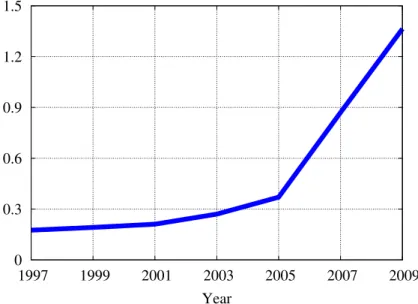
The number of households with reverse mortgages is growing rapidly. Figure 1 shows the proportion of homeowner households of age 65 or above that had reverse mortgages between 1987 and 2009. Both the government-administered HECM loans and private mortgage loans are included. As the figure shows, the use of reverse mortgages was limited before 2000. In 2001, the share of eligible homeowners who had reverse mortgages was about 0.2 percent. This
1This section is based on, among others, AARP (2010), Shan (Forthcoming), Nakajima (Forthcoming), and
information available on the HUD website.
2Many other reverse mortgage products, such as Home Keeper mortgages, which were offered by Fannie Mae,
or the Cash Account Plan offered by Financial Freedom, were recently discontinued, in parallel with the expansion of the HECM market. See Foote (2010).
0 0.3 0.6 0.9 1.2 1.5 1997 1999 2001 2003 2005 2007 2009 Year
Figure 1: Percentage of elderly (age≥65) homeowners with reverse mortgages. Source: AHS.
share increased rapidly since then, reaching 1.3 percent in 2009. Although the level is still low, the growth is all the more impressive if one considers that the popularity of reverse mortgages continued to rise even though the housing market and mortgage markets in general have been stagnating since the beginning of the ongoing housing market downturn.
Reverse mortgages differ from conventional mortgages in six major ways. First, as the name suggests, a reverse mortgage loan works in thereverse way from the conventional mortgage loan. Instead of paying interest and principal and accumulating home equity, reverse mortgage loans allow homeowners to cash out the home equity they’ve accumulated. That is why RMLs are targeted to older households.
Second, government-administered reverse mortgages (HECM loans) have different require-ments than conventional mortgage loans. These mortgages are available only to borrowers age 62 or older,3 who are homeowners and live in their house. 4 Finally, borrowers must have repaid all or almost all of their other mortgages at the time they take out a reverse mortgage. On the other hand, reverse mortgage loans do not have income or credit history requirements, because repayment is promised not based on the borrower’s income but solely on the value of the house the borrower already owns. According to Caplin (2002), reverse mortgage loans are beneficial for elderly homeowners since many of them fail to qualify for conventional mortgage loans because of income requirements.
Third, reverse mortgage borrowers are required to seek counseling from a HUD-approved
3For a household with multiple adults who co-borrow, “age of the borrower” refers to the youngest borrower
in the household.
4Properties eligible for HECM loans are (1) single-family homes, (2) one unit of a one- to four-unit home, and (3) a condominium approved by HUD.
counselor in order to be eligible for a HECM loan. The goal is to be certain that older borrowers understand what kind of loan they are getting and what the potential alternatives are before taking out a reverse mortgage loan.
Fourth, there is no pre-fixed due date; repayment of the borrowed amount is due only when the house is sold and all the borrowers move out, or when all the borrowers die. As long as at least one of the borrowers continues to live in the same house, there is no need to repay any of the loan amount. There is no gradual repayment with a fixed schedule, as with a conventional mortgage loan or line of credit; repayment is made in a lump sum from the proceeds from the sale of the house.
Fifth, HECM loans are non-recourse; borrowers are insured against substantial drops in house prices. Borrowers (or their heirs) can repay the loan either by letting the reverse mortgage lender sell the house, or by repaying. Most use the first option. If the sale value of the house turns out to be larger than the sum of the total loan amount and the various costs of the loan, the borrowers receive the remaining value. In the opposite case, where the house value cannot cover the total costs of the loan, the borrowers are not liable for the remaining amount. The mortgage lender does not have to absorb the loss either, because the loss is covered by insurance, with the premium included as a part of a HECM loan cost structure.
Finally, there are various ways to receive payments from the RML. Borrowers can choose one of five options, and these can be changed during the life of the loan, at a small cost. The options are:
• Tenure: Borrowers continue to receive a fixed amount as long as one of the borrowers continues to live in the same house.
• Term: Borrowers receive a fixed amount for a fixed length of time.
• Line of credit: Borrowers can flexibly draw cash, up to a limit, during a pre-determined drawing period.
• Modified tenure: Combination of the tenure option and the line of credit option. • Modified term: Combination of the term option and the line of credit option.
Of the payment options listed, the line of credit option has been the most popular. HUD reports that the line of credit plan is chosen either alone (68 percent) or in combination with the tenure or term plan (20 percent). In other words, it appears that older homeowners use reverse mortgages mainly to flexibly withdraw cash out of accumulated home equity.
How much can one borrow using a reverse mortgage? Let’s start with the case in which borrowers receive a one-time cash payment under a reverse mortgage. The starting point is the appraised value of the house, but there is a federal limit for a government-administered HECM loan. Currently, the limit is 625,500 dollars for most states.5 The less of the appraised value and 5The limit was raised in 2009 from 417,000 dollars as part of the Housing and Economic Recovery Act of 2008. The 625,500 limit is valid until December 2011.
0 0.01 0.02 0.03 0.04 0.05 0 10 20 30 40 50 60 70 80 90 Initial Principal Limit as a percentage of house value
Figure 2: Initial Principal Limit as a percentage of house value. Source: Shan (Forthcoming). 0 0.02 0.04 0.06 62 67 72 77 82 87 92 97 Age of borrowers
Figure 3: Age of borrowers of reverse mortgage loans. Source: Shan (Forth-coming).
the limit is called the Maximum Claim Amount (MCA).6 Reverse mortgage borrowers cannot receive the full amount of the MCA because there are various costs that have to be paid from the house value as well. There are two types of costs: non-interest costs and interest costs. Moreover, if borrowers have outstanding mortgages, part of the new mortgage loan will be used to pay off the outstanding balance of other mortgages. Non-interest costs include an origination fee, closing costs, the insurance premium, and a loan servicing fee. The insurance premium depends on the value of the house and how long the borrowers live and stay in the same house. More specifically, the insurance premium is 2 percent of the appraised value of the house (or the limit if the value is above the limit) initially and 1.25 percent of the loan balance annually.7 Interest costs depend on the interest rate, the loan amount, and how long the borrowers live and stay in the house. The interest rate can be either fixed or adjustable. In case of an adjustable interest rate, the borrowing interest rate is the sum of the reference interest rate plus margin charged by the mortgage lender, and there is typically a ceiling on how much the interest rate can go up per year or during the life of a loan. The Initial Principal Limit (IPL) is calculated by subtracting expected interest costs from the MCA. The Net Principal Limit is calculated by subtracting various upfront costs from the IPL.
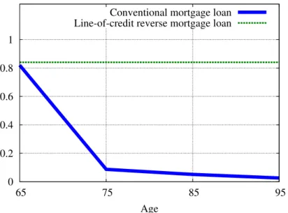
The IPL, which is the amount available for reverse mortgage borrowers at the time of closing, is thus larger the larger the house value, the lower the outstanding mortgage balance, the older the borrower, and the lower the interest rate. Figure 2 shows the distribution of the initial principal limit as a percentage of the house value against which mortgage loans are borrowed. It is clear that many homeowners can borrow around 60 to 70 percent of the appraised house value using reverse mortgages. If the term option is chosen, the total loan amount is divided depending
6Private mortgage lenders offer jumbo reverse mortgage loans, which allow borrowers to cash out more than
the federal limit. However, borrowers have used jumbo reverse mortgages less and less often as the federal limit has been raised.
on the number of times the borrower receives cash. With the tenure option, the amount of cash payment per period is determined by the number of times the borrowers are expected to receive cash.
To understand who the reverse mortgage borrowers are, Shan (Forthcoming) looked at the characteristics of areas with more reverse mortgage borrowers and investigated how those char-acteristics changed over time. She found that areas with more reverse mortgage borrowers tend to have lower household income, higher house value, relatively higher homeowner costs, and lower credit scores. The median house value among reverse mortgage borrowers was 222,000 dollars in 2007, which was about 25 percent higher than the median house value of all older homeowners (175,000 dollars). Figure 3 shows the age distribution of borrowers when they took reverse mortgage loans, during 2003-2007. Observe that there is a spike at age 62, which is the first eligibility age. Shan (Forthcoming) also showed that the distribution is shifting to the right over time, implying that reverse mortgage borrowers got younger, with the spike at age 62 more pronounced.
3
Model
We will set up the decision problem of retired homeowners and renters, based on our previous work (Nakajima and Telyukova (2011)). Renters face a simple decision of consumption, savings, and the size of the house to rent each period, subject to various kinds of shocks. Renters are subject to shocks to health status (including mortality), medical expenditures, and house price. We do not allow renters to buy a house and become homeowners. This assumption is motivated by our data (Health and Retirement Study), in which the proportion of retired households switching from renting to owning is small. Homeowners choose how much to consume and save, and whether to stay in their house or move out and become a renter. Homeowners face the same set of shocks as renters, and, in addition, may exogenously be forced to move out of their house. This shock is intended to capture the deterioration of health and the possibility of moving involuntarily into a nursing home as a result. In addition, homeowners can borrow against their home equity using traditional mortgage arrangements, but this collateral constraint is age-dependent, and tightens with age, as we found in our previous work.
Into this benchmark, we introduce reverse mortgage loans for homeowners. We consider two types of RML’s, namely line-of-credit and tenure options, since they are the most popular ones. We do not model the term option because the more flexible line of credit can perfectly replicate the term option, as long as the pricing is fair. Homeowners utilizing different types of reverse mortgages face different constraints over the life-cycle. In addition, homeowners who utilize reverse mortgages cannot also borrow using a traditional mortgage, which mirrors the restriction of the in the data.
We will characterize the problem recursively. The state space for a household is given by its age i, pension income b, health status m, medical expenditures x, house price p, house size h, financial asset holdingsa, and the type of reverse mortgage j that the household takes, if it is a homeowner.
3.1 Renter’s Problem
We start from describing the renter’s decision problem, the simpler of the two types of house-holds, since renting is the absorbing tenure state. We define the problem recursively. Following convention, we use a prime to denote a variable in the next period. In order to save notation, we useh= 0 to represent a renter. h >0 means that the household is a homeowner with a house size ofh. We use j to denote the type of RML that a household is utilizing. Since reverse mortgages are only available for homeowners, j = 0 for renters. The renter’s problem is as follows:
V(i, j = 0, b, m, x, p, h= 0, a) = max ˜ h∈H,a0≥0 n u(c,h,˜ 0) + β X m0>0 πm,mm 0 X x0 πxi+1,m0,x0 X p0 πp,pp 0V(i+ 1,0, b, m0, x0, p0,0, a0) +βπm,m0v(a0) ) (1) subject to: ˜ c+a0+rh˜hp+xb = (1 +r)a+b (2) c= max{c,˜c} if a0 = 0 and ˜h=h1 ˜ c otherwise (3)
Naturally a renter has no house (h = 0), and no reverse mortgage (j = 0). A renter, taking the states as given, chooses consumption (c), savings (a0), and the size of the house to rent (˜h). (m, x, p) are the shocks. ˜h is chosen from a discrete set H = {h1, h2, ..., hH}, where h1 is the smallest andhH is the largest house available. a0 is assumed to be non-negative. In other words, only home equity borrowing is available in the model. πm
m,m0, πxi+1,m0,x0, and πp,pp 0 denote the
transition probabilities of (m, x, p), respectively. m > 0 indicates health levels, with a higher m indicates better health. Moreover, the transition of m also includes mortality risk; m0 = 0 implies that the renter does not survive to the next period. The current utility of the renter depends on non-housing consumption (c), services generated by the rental property (which are assumed to be linear in the size of the rental property ˜h), and tenure status (o). o= 1 represents ownership while o = 0 indicates renting. The tenure status in the utility function is intended to capture the additional private value of owned housing. The continuation value is discounted by the subjective discount factor β. Following De Nardi (2004), we assume warm-glow bequest motive with utility v(a0).
Equation (2) is the budget constraint for a renter. The left-hand side represents expendi-tures, which consist of consumption (˜c), savings (a0), rent payment (rhtildehp), and medical
expenditures, which are proportional to the level of pension income (xb). rh is the rental rate
for a unit of housing. The right-hand side represents various income, which consists of financial asset holdings and interest income (1 +r)a and pension income b. Equation (3) represents the consumption floor, which is supported by the government. If ˜cimplied in the budget constraint (2) is lower than the consumption floor (c), the household can consume cwith the support from the government, if the household chooses the smallest rental property (h1) and gives up all the savings (a0 = 0).
3.2 Mortgage Choice
We assume that households are born at age 65 (age i = 1 in the model), and those who own a house in the initial period can choose whether to stay in their home or move out. Those who stay can borrow using a reverse mortgage with the line-of-credit option (j = 1), one with the tenure option (j = 2), or not to use a RML at all (j = 0). For now, we do not allow households to obtain or change reverse mortgages later in their life. Formally:
j = arg max
j∈{0,1,2}
V(1, j, b, m, x, p, h, a) (4)
3.2.1 Homeowner’s Problem: No Reverse Mortgage
Here we describe the problem of the homeowner who decides not to take a reverse mortgage. Such a household can also make a tenure decision: to stay a homeowner, or sell and become a renter. Thus, the Bellman equation that characterizes the problem of a homeowner without a reverse mortgage (j = 0) is as follows:
V(i, j = 0, b, m, x, p, h, a) = πni,mV0(i,0, b, m, x, p, h, a) + (1−πi,mn ) max{V0(i,0, b, m, x, p, h, a), V1(i,0, b, m, x, p, h, a)} (5) V1(i,0, b, m, x, p, h, a) = max a0≥−h(1−λi){u(c, h,1) +β X m0>0 πm,mm 0 X x0 πxi+1,m0,x0 X p0 πp,pp 0V(i+ 1,0, b, m0, x0, p0, h, a0) +βπmm,0v(hp+a0) ) (6) subject to: c+a0+xb+hpδ= (1 + ˜r)a+b (7) ˜ r= r if a≥0 r+ιm if a <0 (8) V0(i,0, b, m, x, p, h, a) = max a0≥0 {u(c, h,1) +β X m0>0 πm,mm 0 X x0 πxi+1,m0,x0 X p0 πp,pp 0V(i+ 1,0, b, m0, x0, p0,0, a0) +βπm,m0v(a0) ) (9) subject to (8) and: ˜ c+a0+xb+hp(δ+κ) =hp+ (1 + ˜r)a+b (10) c= max{c,˜c} if a0 = 0 ˜ c otherwise (11)
Equation (5) represents the tenure decision as well as the nursing-home moving shock. With probability πni,m, the homeowner has to move out of the house involuntarily, a shock that will be calibrated based on nursing home transitions in the data. With probability (1− πn
i,m), a
homeowner can choose whether to remain an owner (V1(.)), or voluntarily sell the house and become a renter (V0(.)).
Bellman equation (6) is conditional on remaining a homeowner. The homeowner chooses financial asset holdings for the next period (a0) to maximize the sum of the current utility and the continuation value. Current utility depends on consumption (c), house size (h), and tenure status (o), which is 1 for homeowners. New (m0, x0, p0) are drawn for the next period. As the household remains a homeowner, and chooses no reverse mortgage, it can borrow up to a fixed fraction of the value of the house using a conventional equity loan. a0 ≥ −h(1−λi) is the collateral
constraint; the household can borrow up to (1−λi) of the house value. Age dependence of λi
reflects the fact that it is difficult for elderly homeowners to borrow using conventional home equity loans, as estimated in Nakajima and Telyukova (2011). The household keeps the house in the next period, and the amount of its bequest in case the household does not survive to the next period ishp+a0. Equation (7) is the budget constraint. The left-hand side includes consumption (c), saving (a0), medical expenditures (xb), and the maintenance cost (hpδ). The right-hand side is the same as for renters, consisting of principal and interest income of financial assets ((1 + ˜r)a) and pension income (b). Equation (8) characterizes the interest rate. The saving rate isr, while borrowing interest rate is the saving interest rate plus the conventional mortgage premium ιm.
Bellman equation (9) is conditional on moving out and becoming a renter. There are three differences from equation (6). First, the household becomes a renter in the next period (h0 = 0). Second, if the household does not survive to the following period, its bequest is a0, as the household will have sold the house. Third, since the household is selling the house, it cannot borrow against home equity; thus we have a0 ≥0. Equation (10) is the budget constraint. The house-seller pays the selling cost hpκ, and receives the sale value of the house (hp). Equation (11) characterizes the consumption floor provided by the government. A homeowner becomes eligible for the consumption floor c by selling the housing and decumulating all financial assets to zero.
3.2.2 Homeowner’s Problem: Reverse Mortgage with Line-of-Credit Option
We introduce a stylized version of a reverse mortgage loan with the line-of-credit option, which is characterized by a triplet{λ`, ι`, ν`}. λ` determines the maximum amount as a proportion of the
house value at the time of closing that the borrower can take out. The subscript`represents line-of-credit option. ι` is the margin, or per-period cost proportional to debt balance, in addition
to interest rate. ν` is the upfront cost due at the time of the closing, as a proportion of the
house value. Moreover, the borrower is liable for paying upfront cost νi and annual cost ιi as
the insurance premium against house price shocks. Insurance is mandatory and the premium is determined by the government. Given {λ`, ι`, ν`, νi, ιi}, the problem of homeowners with a
line-of-credit reverse mortgage can be recursively defined as follows: V(i, j = 1, b, m, x, p, h, a) = πni,mV0(i,1, b, m, x, p, h, a) + (1−πi,mn ) max{V0(i,1, b, m, x, p, h, a), V1(i,1, b, m, x, p, h, a)} (12) V1(i,1, b, m, x, p, h, a) = max a0≥−h(1−λ`){u(c, h,1) +β X m0>0 πm,mm 0 X x0 πix+1,m0,x0 X p0 πpp,p0V(i+ 1,1, b, m0, x0, p0, h, a0) +βπm,m0v(w1(i, p, h, a0)) ) (13) subject to: c+a0+xb+hpδ= (1 + ˜r)a+b (14) ˜ r= r if a≥0 r+ι`+ιi if a <0 (15) w1(i, p, h, a0) = max{hp−h(ν`+νi)(1 +r+ι`+ιi)i−1,0}+a0 if a0 ≥0 max{hp−h(ν`+νi)(1 +r+ι`+ιi)i−1+a0,0} if a0 <0 (16) V0(i,1, b, m, x, p, h, a) = max a0≥0 {u(c, h,1) +β X m0>0 πm,mm 0 X x0 πix+1,m0,x0 X p0 πpp,p0V(i+ 1,0, b, m 0 , x0, p0,0, a0) +βπmm,0v(a0) ) (17) subject to (11), (15), (16), and: ˜ c+a0+xb+hp(δ+κ) =w1(i, p, h, a) + ˜ra+b (18)
Equation (12) once again represents the tenure decision. Equation (13) is the Bellman equation conditional on staying in the same house. Since the homeowner utilizes the RML, the collateral constraint is a0 ≥ −h(1−λ`). That is, the reverse mortgage replaces conventional mortgages
for any borrower, mirroring the restriction in the data that an RML borrower cannot have outstanding mortgage debt. Thus, for an RML borrower, the collateral is not age-dependent. The budget constraint (14) is nearly the same as the budget constraint for homeowners without an RML, except for the interest rate applied to borrowing. As defined in equation (15), the margin and the insurance premium (ι` +ιi) are added to the saving interest rate. Equation
(16) defines consolidated wealth in the following period in case the borrower with a line-of-credit reverse mortgage loan does not survive; this captures two distinguishing features of RMLs. First, the upfront cost plus the accumulated interest associated with it (h(ν`+νi)(1 +r+ι`+ιi)i−1) is
deducted from the sales value of the house (hp). Second, the loan is non-recourse, in the sense that if the sales value of the house turns out to be insufficient to cover the upfront cost and the
outstanding debt, the borrower is not liable for the difference. This could happen as the sales price of the house depends on the current price (p), while the borrowing constraint only depends on the price of the house at the time of closing, which is normalized to unity.
The Bellman equation (17) conditional on selling the house is the same as for the homeowner without a reverse mortgage loan. The difference in the budget constraint (18) is that the RML becomes due when the homeowner moves out of the house. In particular,w1(i, p, h, a) represents how the sales value of the house and outstanding reverse mortgage loan with line-of-credit option, if any, is consolidated (equation (16)).
Let us make one remark in terms of modeling the line-of-credit option. The line-of-credit in the model is slightly different from the line-of-credit option in reality. In reality, borrowers do not explicitly pay the interest and the flow costs every period. Instead, the total expected sum of interest and other flow costs is computed at the time of the closing, and the amount is subtracted from the amount of the credit line. Naturally, if a borrower lives and stays in the house for a long time, the actual interest and other flow costs exceed the expected interest payment, and the lender cannot cover the total costs associated with the loan by the sales value of the home. Some of the costs associated with the reverse mortgage must be used to cover such potential loss. In this sense, the line-of-credit option modeled here is more flexible than the real counterpart; the lender does not carry such risk. In other words, the costs associated with the line-of-credit option in the model might be understated (overstated) for the point of view of the mortgage lenders (borrowers).
3.2.3 Homeowner’s Problem: Reverse Mortgage with Tenure Option
The stylized version of the reverse mortgage loan with the tenure option is characterized by a triplet {bt(h), ιt, νt}. bt(h) is the annuity income each period, which depends on the value of
the house in the initial period, when p is normalized to one. The subscript t represents tenure option. As long as the household is alive and lives in the same house of sizeh, the household can receivebt(h). ιt is the margin added to the interest rate. νt is the upfront cost due at the time of
closing. As with other types of reverse mortgages, the borrower is liable for paying upfront cost of νi and the margin ιi as the insurance premium against house price shocks.
Before describing the problem of a homeowner with tenure reverse mortgage, let us discuss the simplifying assumption for the stylized version of the reverse mortgage. In reality, how much a borrower can receive under the tenure option depends not only on the value of the house at the time of the closing (h), but also the outstanding balance of the conventional mortgage loan. This is because when a homeowner takes a reverse mortgage, the outstanding balance of the conventional mortgage loan is repaid using the reverse mortgage and replaced. Therefore, the per-period income under the tenure option is calculated based onh−ainstead ofhin casea <0. However, this incurs a large computational cost as the income under the tenure option depends not only onh but (h, a). To reduce the computational burden, we assume that the conventional mortgage loan must be repaid at the time of the closing of the tenure reverse mortgage loan. Naturally, households with a large outstanding balance of the conventional reverse mortgage loans will not take the tenure option because of it. However, as we mention in Section 2, since a borrower of a reverse mortgage loan has to have repaid all or almost all of the other conventional
mortgage loans, this assumption is not far from reality. Since the existing mortgage loans are repaid at the signing of the reverse mortgage, and the tenure option only provides fixed amount of flow income each period, the borrower cannot borrow under the tenure option, i.e.,a0 ≥0 for alli.
Now, given {bt(h), ιt, νt, νi, ιi}, the problem of homeowners with a tenure reverse mortgage
can be recursively defined as follows:
V(i, j = 2, b, m, x, p, h, a) = πni,mV0(i,2, b, m, x, p, h, a) + (1−πi,mn ) max{V0(i,2, b, m, x, p, h, a), V1(i,2, b, m, x, p, h, a)} (19) V1(i,2, b, m, x, p, h, a) = max a0≥0 {u(c, h,1) +β X m0>0 πm,mm 0 X x0 πix+1,m0,x0 X p0 πpp,p0V(i+ 1,2, b, m0, x0, p0, h, a0) +βπm,m0v(w2(i, p, h, a0)) ) (20) subject to: c+a0+bx+hpδ= (1 +r)a+b+bt(h) (21) w2(i, p, h, a0) = max ( hp−h(νt+νi)(1 +r+ι`+ιi)i−1− i X k=1 (1 +r+ιt+ιi)k−1bt(h),0 ) +a0 (22) V0(i,2, b, m, x, p, h, a) = max a0≥0 {u(c, h,1) +β X m0>0 πm,mm 0 X x0 πix+1,m0,x0 X p0 πpp,p0V(i+ 1,0, b, m 0 , x0, p0,0, a0) +βπmm,0v(a0) ) (23) subject to (11), (22) and: ˜ c+a0+xb+hp(δ+κ) =w2(i, p, h, a) +ra+bt(h) (24)
Equation (19) characterizes the tenure choice as well as the move-out shock. Equation (20) is the Bellman equation conditional on remaining a homeowner. The budget constraint includes the extra pension incomebt(h) which is associated with the tenure reverse mortgage. Moreover,
since households can only save under the tenure option, the interest rate is always r. Equation (22) defines how the assets and debts are consolidated in the case of death. The first term (hp) is the sales value of the house. The second term (h(ν`+νi)(1 +r+ι`+ιi)i−1) denotes the upfront
cost plus accumulated interest and flow costs associated with it. The third term is the sum of all pension income together with accrued interests (r), and premiums and fees (ιt+ιi). The pension
which is the last period in which the borrower received the pension income under the tenure reverse mortgage. The borrower is not liable for the loss if the sum of the three terms turns out to be negative. This happens when the house price is so low, or the borrower lives and receives the pension income for long. Notice thata is outside the max operator.
Equation (23) is the Bellman equation conditional on moving out and becoming a renter. The budget constraint (21) includes the additional pension income (bt(h)) and the consolidated
asset balance (computed based on equation (22)).
To conclude this section, let us discuss the trade-offs among mortgage choices. There are two benefits of taking a reverse mortgage. First, since the collateral constraint associated with con-ventional mortgages tightens as households age, reverse mortgages allow homeowners to access home equity when it becomes difficult to do through other means. Second, reverse mortgages protect homeowners from house price risk, since reverse mortgages are non-recourse loans. More-over, reverse mortgages with the tenure option provide additional insurance against longevity. The costs of the RML are the fixed upfront cost and interest premia. For example, if a household takes a reverse mortgage loan, and is forced to move out right after taking it, the household is liable for the fixed cost without enjoying the benefits of reverse mortgage loans. The line-of-credit and tenure options combine these costs and benefits in different ways. The line-of-line-of-credit option gives homeowners the ability to borrow flexibly according to their needs, and so long as they don’t use the line of credit, borrowers do not need to pay for the interest and other flow costs. Instead, the tenure option provides partial insurance against longevity risk, but the interest costs acumulate inflexibly in our model, which can be detrimental when borrowers are relatively young and don’t need the extra income. We use the calibrated version of the model to analyze the trade-offs quantitatively.
For now, we focus below only on the line-of-credit option, which is by far the most popular.
4
Calibration
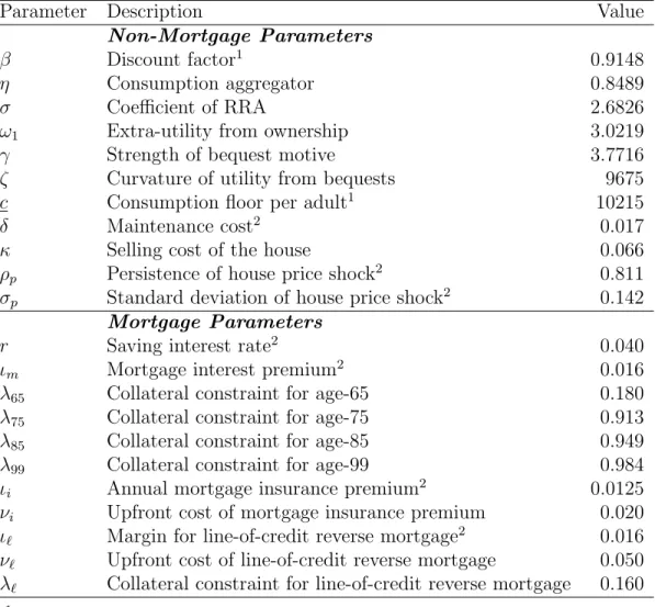
In order to calibrate the model, we use a two-step estimation procedure, where in the first step we calibrate all the parameters exogenous to the model, and in the second step, estimate the rest of the parameters to match relevant lifecycle facts. Since the model employed in this paper is based on Nakajima and Telyukova (2011), we use the parameter values estimated by our previous work whenever reasonable. There, the facts employed in the second step of the estimation are the lifecycle profiles of homeownership rates, net worth, housing versus nonhousing assets, and home equity debt among retirees, all estimated in the data from the Health and Retirement Study (HRS) over the period 196-2006. One model period is set to two years. Households are born in the model at age 65, and can live up to 99 years of age. Table 1 summarizes the calibrated parameter values; below we discuss the details.
4.1 Preferences
Households use discount factorβ to discount future value. The following period utility function with constant relative risk aversion is used.
u(c, h, o) = (c
η(ω
oh)1−η)
1−σ
Table 1: Calibration Summary
Parameter Description Value
Non-Mortgage Parameters
β Discount factor1 0.9148
η Consumption aggregator 0.8489
σ Coefficient of RRA 2.6826
ω1 Extra-utility from ownership 3.0219
γ Strength of bequest motive 3.7716
ζ Curvature of utility from bequests 9675
c Consumption floor per adult1 10215
δ Maintenance cost2 0.017
κ Selling cost of the house 0.066
ρp Persistence of house price shock2 0.811
σp Standard deviation of house price shock2 0.142
Mortgage Parameters
r Saving interest rate2 0.040
ιm Mortgage interest premium2 0.016
λ65 Collateral constraint for age-65 0.180
λ75 Collateral constraint for age-75 0.913
λ85 Collateral constraint for age-85 0.949
λ99 Collateral constraint for age-99 0.984
ιi Annual mortgage insurance premium2 0.0125
νi Upfront cost of mortgage insurance premium 0.020
ι` Margin for line-of-credit reverse mortgage2 0.016
ν` Upfront cost of line-of-credit reverse mortgage 0.050
λ` Collateral constraint for line-of-credit reverse mortgage 0.160
1 Biennial value. 2 Annualized value.
η is the Cobb-Douglas aggregation parameter between non-housing consumption goods (c) and housing services (h). σ is the risk aversion parameter. ωo represents the extra utility attached to
housing that households already own. For renters (o = 0), ω0 is normalized to unity. For home-owner (o= 1), ω1 >1 represents nonfinancial benefits of homeownership, such as attachment to one’s house and neighborhood, as well as financial benefits not captured explicitly by the model, such as tax benefits and insurance against rental rate fluctuation.
A household gains utility from leaving bequests. When a household dies with the consolidated wealth of a, the household’s utility function takes the form:
v(a) =γ(a+ζ) 1−σ
1−σ . (26)
Table 2: Income Levels1
Group Group 1 Group 2 Group 3 Group 4 Group 5
Income 5831 12049 17844 25868 50227
1 Annualized income in 1996 dollars. Source: HRS 1996 wave.
The parameters associated with the preference are taken from the baseline estimate of Naka-jima and Telyukova (2011). We obtained β = 0.9148, η = 0.8429, σ = 2.6826, ω1 = 3.0219, γ = 3.7716, and ζ = 9,675. These estimates are discussed in detail in that paper.
4.2 Nonfinancial Income
We use five levels of nonfinancial income. Table 2 summarizes five nonfinancial income bins. Our definition of nonfinancial income includes Social Security, pension, disability, annuity, and government transfer income. Because some of our retirees are only partly retired, we also in-clude labor income in this measure. However, labor income plays a small role in our sample, constituting on average about 6% of total income. Following Nakajima and Telyukova (2011), we adjust income of two-adult households by dividing the income by 1.5. This factor is obtained by computing the drop in income when the number of adults in a household drops from two to one in HRS. We compute the nonfinancial income of households of age between 63 and 67 in 1996 HRS sample, sort them, allocate them into five bins equally, and compute the median income in each quintile.
4.3 Consumption Floor
The consumption floor c supported by the government through various welfare programs is estimated together with other parameters in our previous work (Nakajima and Telyukova (2011)). We estimated c = 10,215 in 1996 dollars, which aligns well with empirical estimates of such program benefits (Hubbard et al. (1994)).
4.4 Health Status and Mortality Risk
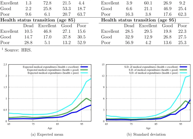
As in Nakajima and Telyukova (2011), we group the five self-reported health status categories in the HRS into three categories: excellent, good, and poor. We also add death as one of the health states. Then we compute the transition probabilities across health states, including probability of death, using the HRS sample pooled across all waves. Table 3 shows the resulting transition probabilities for people of age 65, 75, 85, and 95.
4.5 Medical Expenditures
As in Nakajima and Telyukova (2011), we estimate the distribution of out-of-pocket medical expenditures as a proportion of income, conditional on age and health status. First, we compute the probability that medical expenditures are zero in a given period, conditional on age and health status. Then we estimate the mean and standard deviation of medical expenses as a share of income, assuming a log-normal distribution, also conditional on age and health state.
Table 3: Health Status Transition (Percent)
Health status transition (age 65) Health status transition (age 75)
Dead Excellent Good Poor Dead Excellent Good Poor
Excellent 1.3 72.8 21.5 4.4 Excellent 3.9 60.1 26.9 9.2
Good 2.2 25.8 53.3 18.7 Good 6.6 21.1 46.9 25.4
Poor 9.6 6.1 20.7 63.7 Poor 16.3 3.8 17.6 62.3
Health status transition (age 85) Health status transition (age 95)
Dead Excellent Good Poor Dead Excellent Good Poor
Excellent 10.5 46.8 27.1 15.6 Excellent 28.5 29.5 19.8 22.3 Good 14.7 17.0 37.8 30.5 Good 32.9 12.9 26.8 27.5 Poor 28.8 5.1 13.2 52.9 Poor 56.9 4.2 13.6 25.3 1 Source: HRS. 0 0.5 1 1.5 2 2.5 65 75 85 95 Age
Expected medical expenditures (health = excellent) Expected medical expenditures (health = good) Expected medical expenditures (health = poor)
(a) Expected mean
0 3 6 9 12 15 65 75 85 95 Age
S.D. of medical expenditures (health = excellent) S.D. of medical expenditures (health = good) S.D. of medical expenditures (health = poor)
(b) Standard deviation
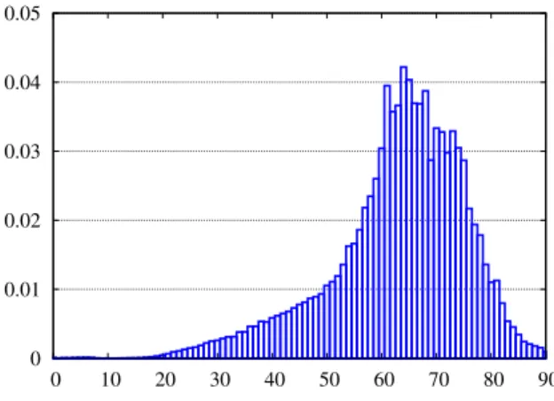
Figure 4: Distribution of out-of-pocket medical expenditures. Source: HRS.
Figure 4 exhibits the resulting mean and standard deviation. Unsurprisingly, both are high for the less healthy and the older, and increase particularly dramatically for the oldest old.
4.6 Involuntary Nursing Home Moves
Using the HRS, we compute the 2-year probability that a household moves into a nursing home, conditional on the household’s age and health status. Table 4 shows the probabilities for age 65, 75, 85, and 95. We interpret the event of moving into a nursing home as compulsory moves out of the house, which are important when considering a loan which depends critically on how long a household stays in the house. Not surprisingly, the probability is generally higher for older and less healthy households. There are two caveats to these estimates. First, not all elderly move into nursing homes involuntarily. If we take into account that some of the moves are voluntary, the
Table 4: Probability of Moving to Nursing Home (Percent)
Health status
Age Excellent Good Poor
65 0.15 0.30 0.86
75 0.59 1.47 3.03
85 5.16 7.66 11.19
95 25.32 22.07 25.13
1 Source: HRS.
Table 5: House Size Bins1
Bin 1 2 3 4 5 6 7 8 9 10
Size 21792 44935 63613 77839 88087 101358 125114 152107 195244 360683
1 Value in 1996 dollars. Source: HRS.
probability that a household is forced to move out is upward-biased. On the other hand, some older retirees might move to their children’s homes instead of a nursing home. This consideration implies that the probability of a moving shock might be underestimated. Since the data limit how well we can identify these events, we consider our estimates of the moving shock to be reasonable.
4.7 Housing
We create 10 house size bins, by sorting house values of all homeowners of age 63-67 in 1996 HRS sample, equally allocating them into 10 bins, and computing the median value of each bin. Housing requires maintenance, whose cost is a fractionδof the house value. δis set at 1.7 percent per year, which is the average depreciation rate of residential structures in National Income and Product Accounts (NIPA). When a household sells the house, the sales cost, which is a fraction κ of the sales price, has to be paid. The selling cost of a house (κ) is set at 6.6% of the value of the house. This is the estimate obtained by Greenspan and Kennedy (2007). Grueber and Martin (2003) report the median selling cost of 7.0% of the value of the house. Rent is the sum of maintenance costs (δ) and the conventional mortgage interest rate (r+ιm).
To calibrate idiosyncratic house price shocks, we assume that the house price is normalized to one in the initial period, and follows an AR(1) process thereafter. Contreras and Nichols (2010) estimate the AR(1) process of house prices for nine Census regions as well as the U.S. as a whole Their estimate of the persistence parameter associated with the Census regions varies between 0.704 and 0.940. Their estimate for the national sample is 0.811, which we use as our persistence parameter. Their estimates for the standard deviation of the shocks from Census regions varies between 6.5 percent and 9.3 percent, while the estimate from the national sample is 7.9 percent. On the other hand, Flavin and Yamashita (2002) estimate the standard deviation of individual house prices using Panel Study of Income Dynamics (PSID) and obtain the standard deviation
0 0.2 0.4 0.6 0.8 1 65 75 85 95 Age
Conventional mortgage loan Line-of-credit reverse mortgage loan
Figure 5: Collateral constraint as a proportion of house value.
of 14.2 percent. We use 14.2 percent as our standard deviation to house price shocks, since the shock in our model is associated with individual house value. The AR(1) process is discretized into a first-order Markov process. Since one period in the model spans two years, while the house price shocks constructed above are at annual frequency, we square the obtained Markov process to make it into a biennial process.
4.8 Mortgage Loans
The interest rate is set at 4% per year (8% biennially). For conventional mortgage loans, we assume a borrowing premium of 1.6% annually. This is the average spread between 30-year conventional mortgage loans and Treasury bills of the same maturity between 1977 and 2009. The age-dependent collateral constraint for conventional mortgages is characterized by{λi}. We
pin down λi for age 65, 75, 85, and 99 and linearly interpolate the values between these ages.
Estimates of Nakajima and Telyukova (2011) for ages 65, 75, 85, and 99 are 0.18, 0.91, 0.95, and 0.98, respectively. The profile implies that the collateral constraint tightens quickly for the elderly, consistent with the fact that retired households fail income requirements inherent in most equity borrowing contracts (Caplin (2002)). Figure 5 shows {λi}Ii=1.
To calibrate the RML contract, we rely on the contracts in the data and set most parameters exogenously. The upfront and per-period costs associated with insurance against house price shocks are νi = 0.02, and ιi = 0.0125 per year, respectively. The reverse mortgage with
line-of-credit option is characterized by a triplet{λ`, ι`, ν`}. The upfront cost is set at 5% of the house
value. This is the sum of the origination fee and the closing cost. The origination fee is typically 2 percent of the house value up to 200,000 dollars and 1 percent above it, with the cap of 6,000 and the floor of 2,500. Considering that most house values in the model are below 200,000, but half of the houses are below 100,000, where the floor of 2,500 dollars binds, 2.5 percent is reasonable. The closing cost is typically around 2,000 −3,000. Dividing the amount by the
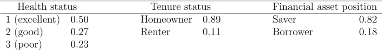
Table 6: Selected Characteristics of the Initial Distribution, Age 65, 1996
Health status Tenure status Financial asset position
1 (excellent) 0.50 Homeowner 0.89 Saver 0.82
2 (good) 0.27 Renter 0.11 Borrower 0.18
3 (poor) 0.23
median house value in the sample, 2.5 percent is the reasonable number. The sum of the two yieldsν` = 0.05. The borrowing limit as a proportion of house value (λ`) is calibrated to match
the observed take-up rate of 1.3 percent. The value we estimate is about 16%, implying that any elderly household can borrow up to 84% of its housing equity through the reverse mortgage. This is in line with the equity limits we see in the data. Figure 5 compares the collateral constraint under the line-of-credit reverse mortgage and the conventional mortgage. It is clear that the former provides a comparatively lax borrowing constraint, especially for older households. As for the interest margin, we set the margin for the line-of-credit reverse mortgages the same as for the conventional mortgage loans, i.e.,ι` = 0.016.
4.9 Initial Type Distribution
The type distribution of age-65 households is constructed using the HRS. Table 6 exhibits some dimensions of the initial distribution. Half of the households are in excellent health. Homeown-ership rate is close to 90 percent. And most of them are in net positive financial asset position. In other words, their total wealth (net of all the debt) is above the value of their house.
5
Results
5.1 Life-Cycle Profiles without Reverse Mortgages
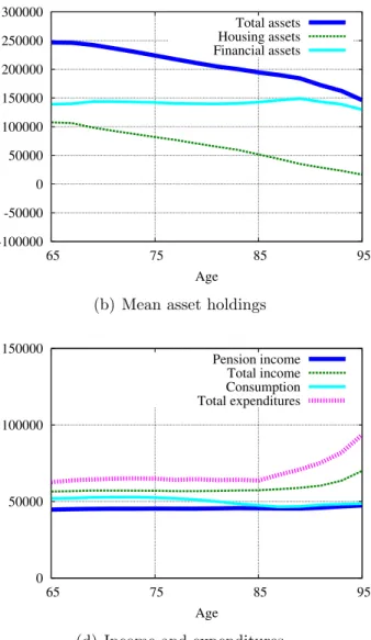
We begin by describing the properties of the model without reverse mortgage loans, to have a benchmark against which to judge the changes that reverse mortgages introduce into the economy. Figure 6 exhibits the relevant life-cycle profiles of retirees. In panel (a), homeownership rate is 89 percent for 65-year-old households, and gradually declines with age, as in the data. Panel (b) shows life-cycle profiles of mean total assets, further broken down into mean housing assets and mean financial (non-housing) assets. In the mean, households decumulate asset holdings very slowly, starting from about 250,000 dollars at age-65 to 150,000 dollars at age-95. We analyze in detail the reasons for the lack of dissaving in this model in Nakajima and Telyukova (2011); we show that slow asset decumulation is characteristic of homeowners, but not renters, and homeowners are motivated by a combination of bequest motives, financial and nonfinancial benefits of homeownership, medical expense risk earlier in the retirement spell and large medical expenses late in life. Panel (c) shows the proportion of households in debt. Consistent with the data, it declines from 17 percent at age-65 to below 1 percent at age-95, as households repay the existing collateralized loans or sell their house and become renters. Panel (d) exhibits income and expenditures. The life-cycle profiles of pension income and consumption are approximately flat. Total expenditures go up sharply towards the end of households’ life as the average medical
0 0.25 0.5 0.75 1 1.25 1.5 65 75 85 95 Age Homeownership rate
(a) Homeownership rate
-100000 -50000 0 50000 100000 150000 200000 250000 300000 65 75 85 95 Age Total assets Housing assets Financial assets
(b) Mean asset holdings
0 0.05 0.1 0.15 0.2 0.25 65 75 85 95 Age Proportion in debt (c) Proportion in debt 0 50000 100000 150000 65 75 85 95 Age Pension income Total income Consumption Total expenditures
(d) Income and expenditures
0 0.02 0.04 0.06 0.08 0.1 0.12 65 75 85 95 Age Movers: total Movers: Voluntary Movers: Shock
(e) Proportion of movers
0 0.25 0.5 0.75 1 1.25 1.5 65 75 85 95 Age
Baseline: Homeownership rate RML: Homeownership rate
(a) Homeownership rate
0 0.2 0.4 0.6 0.8 1 65 75 85 95 Age
Baseline: Proportion in debt RML: Proportion in debt (b) Proportion in debt -10000 0 10000 20000 30000 65 75 85 95 Age
Baseline: Housing assets Baseline: Financial assets RML: Housing assets RML: Financial assets
(c) Mean housing and financial assets
0 5000 10000 15000 20000 25000 30000 65 75 85 95 Age
Baseline: Total assets RML: Total assets
(d) Mean total assets
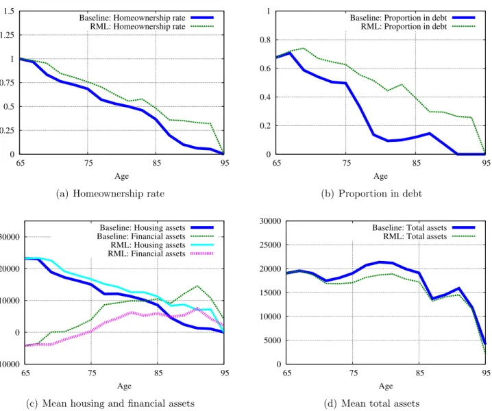
Figure 7: Changes in the life-cycle profiles of reverse mortgage borrowers
expenditures balloon. Income increases in parallel as more households are forced to rely on the consumption floor, and receive the associated transfers. Finally, panel (e) shows the proportion of homeowners who move out of their house at each age. For relatively younger retirees, most households move out voluntarily. As households age, they are increasingly forced to move out into nursing homes. This figure indicates that the worst realization associated with taking a RML – namely, borrowing and immediately moving out of the house involuntarily – is not common for those who take reverse mortgage loans at an earlier age, but becomes more of a threat later on.
5.2 Life-Cycle Profiles with Reverse Mortgages
Figure 7 shows how the life-cycle profiles of households who take line-of-credit RMLs change. Here we track only the life-cycle profiles of the households who, when given the option, borrow against a RML. Panel (a) shows that reverse mortgage loans allow the borrowers to remain
Table 7: Take-up Rate of RMLs, Share of Homeowners Data1 All households 1.36 Model All homeowners 1.37 No outstanding mortgages 0.55 With outstanding mortgages 4.74
Low income 7.13
Medium income 0.18
High income 0.19
Poor health 1.69
Excellent health 0.73
1 2009 American Housing Survey.
in the house longer, which appears as higher homeownership rate in the economy with RMLs. Obviously, these households extract more home equity, which is shown in panel (b). For example, at age 85, 40% of reverse mortgage borrowers have a negative balance of mortgage loans, while only 10% of the same households would have borrowed at the same age without the RML option. Panel (c) exhibits mean housing and financial asset profiles of the RML borrowers. Mean housing asset holdings in the economy with RMLs are greater than in the economy without, which just reflects the higher homeownership rate that results from the introduction of RMLs. On the other hand, in the economy with RMLs, households hold fewer financial assets, or more debt, on average. Panel (d) shows the profile of mean total assets. With reverse mortgage loans, borrowers can decumulate their assets faster, especially between ages 75 and 85, when many of them still want to hold on to their house, but they have higher risks of poor health, high medical expenses, and compulsory moving.
5.3 Benefits of Reverse Mortgage Loans
Table 7 compares the take-up rate of the model and the data. The overall take-up rate, which is 1.4% among all homeowners, is matched well by the model. This is a result of our calibration strategy, which targets this magnitude. Since the homeownership rate is about 89 percent at age-65 in the HRS, this take-up rate translates to 1.2% of all households of age 65 and above.
The table also shows the breakdown of household types to analyze which households are more likely to take an RML. Reverse mortgages are far more popular among homeowners with out-standing mortgages (4.74% takeup rate, versus 0.55% among households with no mortgage debt), low income (7.13% versus 0.2% for higher income groups), and in poor health (1.69% against 0.7% for households in good health). These characteristics of RML borrowers are qualitatively
Table 8: Welfare Gain from Reverse Mortgages
Welfare gain1
All households 4
RML borrowers 292
consistent with the data, although it is hard to get comparable numbers in the data since we do not have micro-data on reverse mortgages. The picture that emerges is that households are likely to use RMLs to repay outstanding mortgage debt and to pay for medical expenses, when their income is insufficient to cover these needs in other ways.
Table 8 quantifies the welfare gain from the availability of reverse mortgages. The welfare gain is measured as the one-time transfer at age 65, in 2010 U.S. dollars , that would make households in the economy without RMLs indifferent to being in the economy with RMLs. Among those who take reverse mortgages when they are available, the welfare gain is equivalent to a one-time transfer of $292. This translates to 1.6% of median pension income of the sample households, and averages out to just $5 per household for all households. The small welfare gain is not surprising given the low take-up rate. Our analysis below is on the reasons for such low take-up rate, and we will revisit the reasons for the low welfare gains as well.
5.4 What Is Behind the Low Take-Up Rate? The Role of Bequest Motives and Uncertainty
In this section, we investigate which elements of the retirees’ environment and behavior contribute to the low RML take-up rate. In particular, we focus on the role of different types of uncertainty that retirees face, and then on the role of bequest motives. Table 9 shows the take-up rate among homeowners in the model with several counterfactual experiments, as well as the associated welfare gains for RML borrowers, measured as before. First, we evaluate the model without medical expenditure shocks; to do this, we assume that all households have to pay the mean of the medical expenditure distribution in the baseline specification. In this case, the take-up rate drops to less than 1%, all other things equal. If we shut off medical expenditures altogether, no household takes reverse mortgage loans. These experiments demonstrate that in the baseline specification, households use reverse mortgages exclusively to pay for medical expenses while staying in their homes. As for welfare gains, without medical expense risk, the welfare gain from RMLs rises to $387 per borrower household. This would average to just $3.4 per household overall.
If the compulsory moving shocks are turned off, the take-up rate of reverse mortgages rises to 4.3 percent of homeowners. This result confirms the result in Michelangeli (2010) that the risk of involuntarily moving into nursing homes contributes to low RML demand. The worst outcome for RML borrowers is to face the compulsory moving shock after paying the large upfront cost of a reverse mortgage, but before utilizing the line of credit. This outcome is eliminated if moving shocks are turned off, which makes reverse mortgages more attractive. In this case, the welfare gain among RML borrowers is $267 per household, or $10 per household when split among all
Table 9: Impact of Uncertainty and Bequest Motives on RML Demand
Take-up rate, Welfare gain, homeowners RML borrowers
Baseline model 1.37 292
No medical expense risks 0.98 387
No medical expenses 0.00 0
No moving shocks 4.28 267
No house price shocks 3.79 243
Expected house price boom 42.80 3243
No bequest motive 59.06 4081
Use of RMLs
No house price shocks, no medical expenses 0.00 0
No moving shocks, no medical expenses 0.10 247
No bequest motive, no medical expenses 68.00 7144
1 Welfare gain is measured by one-time transfer at age 65, in 2010 dollars, that equate life-time utility of those with access to RMLs to those without.
households in the economy.
Similarly, if the house price shocks are turned off, the take-up rate increases to 3.8% of homeowner households. This increase might be counterintuitive at first sight, because one of the benefits of RMLs is their non-recourse nature. However, temporary house price shocks work in the same way as moving shocks. If a household observes a temporary increase of the house value, it may want to sell the house for the capital gain, even though holding on to the house gives extra utility. This implies that the expected duration of tenure as a homeowners is shorter with house price shocks, and thus the value of reverse mortgages is lower. If the house price shocks are eliminated, homeowners remain in their house longer, which makes reverse mortgage more attractive. The welfare gains in the world without house price shocks are $243 per RML borrower.
Next, we add to the model the expectation of house price growth of 4.5% per year, which is the average real house price appreciation rate between 1996 and 2006. In this experiment, the take-up rate rises above 40 percent. This is intuitive: when households expect house price growth, they want to front-load consumption by borrowing more, which can be achieved by taking reverse mortgages. In this case, the welfare gains for RML borrowers rise significantly, to $3243 per borrower household, or $1239 per household overall. This experiment suggests that the observed fast increase in the take-up rate in the period 2000-2009, shown in Figure 1, might be the result of expected house price appreciation.
Table 10: Reverse Mortgage Loans with Alternative Terms – Take-Up Rates, Home-owners
Among all homeowners
Baseline model 1.37
HECM Saver (0.01% upfront insurance cost) 4.20
Lower (0.5%) flow insurance premium 6.35
No insurance (recourse) 14.58
the RML take-up rate increases to about 60% of homeowners. As discussed in the literature on the retirement saving puzzle, including our previous work (Nakajima and Telyukova (2011)), bequest motives are an important element in accounting for the observed slow decumulation of assets among the elderly, and thus it is intuitive that they significantly dampen RML demand. Without bequest motives, many households decumulate assets substantially faster, and reverse mortgages allow them to do so without moving out of the house. Notice that in this case, the magnitude of the welfare gain to RML borrowers from the availability of reverse mortgages is also very large compared to the benchmark case.
In the last set of experiments, we investigate in more detail how households in the model use reverse mortgages. As we established, in the baseline model homeowners use RMLs only to pay for medical expenses. However, we also showed that some features of the environment dampen RML demand significantly. We want to evaluate to what extent, without these features, homeowners begin to use reverse mortgages for non-medical consumption. In the last three rows of table 9 , we answer this question by shutting off medical expenses in the model without house price shocks, moving shocks, and bequest motives. In the world without moving shocks, 0.1% of homeowners use RMLs for non-medical consumption. The dramatic result comes in the world without bequest motives: here, 68% of households use RMLs for non-medical consumption. This explains the large welfare gains from RML loans that we documented above. Notice also that this take-up rate is higher than in the model without bequest motives but with medical expenses. This happens because medical expense shocks create a precautionary motive, which dampens RML demand even in the case without bequest motives; households decumulate assets more slowly in anticipation of large medical expense shocks.
5.5 The Impact of Reverse Mortgage Terms on RML Demand
In this section, we explore how the demand for reverse mortgage loans is affected by their current terms. Table 10 summarizes the results. First, we consider the impact of a change in RML terms introduced in October 2010 by the Federal Housing Administration. The FHA introduced a new type of RML known as the HECM Saver. In order to reduce upfront costs of reverse mortgage loans, often criticized in the popular media for the low RML demand, the HECM Saver only requires upfront insurance premium of 0.01% of house value, down from 2%. However, since a lower insurance premium exposes the government to larger house price risk, the amount of equity