Inferring Network-Wide Quality in
P2P Live Streaming Systems
Xiaojun Hei
†, Yong Liu
‡and Keith W. Ross
†∗†
Department of Computer and Information Science
‡
Department of Electrical and Computer Engineering
Polytechnic University, Brooklyn, NY, USA 11201
[email protected], [email protected] and [email protected]
Abstract— This paper explores how to remotely monitor
network-wide quality in mesh-pull P2P live streaming systems. Peers in such systems advertise to each other buffer maps which summarize the chunks of data that they currently have cached and make available for sharing. We show how buffer maps can be exploited to monitor network-wide quality. We show that information provided in a peer’s advertised buffer map correlates to that peer’s viewing-continuity and startup latency. Given this correlation, we can remotely harvest buffer maps from many peers and then process the harvested buffer maps to estimate ongoing quality. After having developed this methodology, we apply it to a popular P2P live streaming system, namely, PPLive. To harvest buffer maps, we build a buffer-map crawler and also deploy passive sniffing nodes. We process the harvested buffer maps and present results for network-wide playback continuity, startup latency, playback lags among peers, and chunk propagation. The results show that this methodology can provide reasonable estimates of ongoing quality throughout the network.
Index Terms—
I. INTRODUCTION
P2P live streaming systems, using mesh-pull (also known as data-driven and BitTorrent-like) architectures, have enjoyed many successful deployments to date. These deployments include CoolStreaming, PPLive, PPStream, UUSee, SopCast, Boiling-Point-TV, VVSky, TVAnt, QQLive, TVkoo and many more [1], [2], [3], [4], [5], [6], [7], [8], [9], [10]. These systems have mostly originated from China; however, they have a significant user base in Europe and North America [11], [12], [13]. We will likely see continued growth in P2P live streaming over the Internet. In the upcoming years, we can expect these systems to distribute more international television channels, reaching larger and more diverse audiences. Moreover, thanks to the low distribution cost of P2P streaming, we also expect user-generated live video content (emanating from web cams and wireless devices) to be distributed using P2P mesh-pull architectures. A video channel in a P2P live streaming system may be simultaneously watched by thousands or even millions of users from all corners of the world.
In this paper, we explore how to monitor the network-wide quality in a mesh-pull P2P live streaming system. Quality metrics include video playback continuity, initial startup la-tency, and display lags among users. Numerous parties have an interest in monitoring quality:
• The users’ viewing experience is crucial for successful
service deployment. If users experience frequent freezes in the video playback, significant delays for startup after switching channels, or significant time lags among users for the same video frame, then the users may abandon the service. Service providers would like to detect when ser-vice quality degrades, so that they can add, retroactively and dynamically, additional uploading capacity, either using servers that they operate or CDN servers. When service quality is satisfactory, the infrastructure capacity can be released for other purposes.
• In order to compare the service quality of different
channels across different P2P streaming providers, third-party companies will want to independently monitor the channels. This information could then be provided to users as an aid in selecting P2P video providers. It could also be provided to advertisers who wish to advertise in the systems.
• Given the knowledge of the actual performance of the
streaming systems, ISPs and CDNs can dimension their networks and expand capacity more efficiently, attracting more residential and corporate customers.
• Finally, from a research perspective, monitoring P2P live
streaming systems allows researchers to gain an in-depth understanding of various system design choices, includ-ing algorithms for creatinclud-ing peerinclud-ing partners, schedulinclud-ing algorithms (for both uploading and downloading), video encoding algorithms, and so on. Such insights will guide the design of future P2P live streaming systems. The most direct approach to monitoring network-wide quality is to include quality monitors in each of the peers (for example, within the P2P software). Each monitor would determine when media objects arrive at the peer and report this information to a central processing. Based on the sequence of arrival times, the central processing node could estimate quality metrics such as freezing and start up latencies at each of the nodes (see Section IV), and finally combine this information across nodes to obtain network-wide quality measures. But this requires the installation (or integration) of monitors in the peers, which is only possible with direct control of the P2P live streaming system. Without this control, it is a challenging problem to monitor the quality of thousands
of peers scattered around the world.
In this paper, we examine the problem of remotely monitor-ing network-wide quality P2P mesh-pull live streammonitor-ing sys-tems. Similar to BitTorrent, peers in P2P mesh-pull streaming systems advertise to each other the availability of the chunks of data that they currently have cached. These advertisements are called buffer maps. We show how these buffer maps can be exploited to monitor network-wide quality. In particular, we show that the information provided in a peer’s advertised buffer map correlates with that peer’s viewing-continuity qual-ity and startup latency. Given this correlation, we can remotely harvest buffer maps from many peers and then process these buffer maps to estimate ongoing quality metrics.
After having developed the methodology, we apply it to a popular P2P live streaming system, namely, PPLive. Harvest-ing buffer maps from PPLive is in itself a challengHarvest-ing problem, since PPLive is a proprietary protocol. To harvest buffer maps, we develop a buffer-map crawler and also deploy passive sniffing nodes. We process the harvested buffer maps and present results for network-wide playback continuity, startup latency, playback lags among peers, and chunk propagation. The results show that this methodology can provide reasonable estimates of ongoing quality throughout the network. Although our experiments are with PPLive, the methodology can in principle be used for any mesh-pull P2P live streaming system. This paper is organized as follows. We end this section with a summary of related work. In Section II, we provide an overview of mesh-pull systems. In Section III, we present our methodologies for harvesting buffer maps from a mesh-pull P2P streaming system. In Section IV, we demonstrate a strong correlation between the chunk availability reported in buffer maps and the streaming service quality. When apply this buffer methodology to PPLive. In Section V, we use the methodology to estimate network-wide video quality in PPLive, including playback continuity, startup latency, and playback lags. In Section VI, we present results on network-wide chunk propagation. Finally we conclude in Section VII. A. Related Measurement Work on Mesh-pull Streaming Sys-tems
Video quality is conventionally characterized by video dis-tortion; the quality measurement normally involves the video rate measurement from which video distortion is estimated utilizing empirical rate-distortion curves or various proposed rate-distortion models [14]. However, this approach usually varies among the video sequences, and is not suitable for video quality measurement over the Internet [15], [16], [17], [18], [19], [20].
Video quality measurements over the Internet typically involve extensive video traffic measurements [15], [16], [17], [18], [19], [20]. In contrast, our approach does not process video directly, but instead employs buffer maps, which sum-marize the availability of video data at the various peers. This approach generates significantly less measurement traffic in the network.
There have been a few measurement studies in quantifying large scale P2P streaming systems. The measurement tech-niques fall into two categories: passive sniffing and active
crawling. For passive sniffing, our previous work [11] is the first measurement study of a large-scale P2P streaming system. It considered traffic patterns and peer dynamics of the PPLive IPTV system. Our work was followed by two other passive measurement studies [13] and [21]. Ali et al. [13] focus on the traffic characteristics of controlled PPLive peers on PPLive and SopCast. Passive sniffing was also utilized to study the traffic pattern of PPLive, PPStream, TVAnts and SopCast in [21].
Passive sniffing techniques are often constrained to measure a small set of controlled peers. To understand network-wide peer churn dynamics, we developed active crawling apparatus to measure the global view of the PPLive network [12]. Subsequently, another crawler-based measurement study was conducted in [22]. Vu et al. [22] examine the peer dynamics for a small number of PPLive channels.
II. OVERVIEW OFMESH-PULLP2P LIVESTREAMING
SYSTEMS
Mesh-pull streaming systems (including PPLive [2], PP-Stream [3] and CoolPP-Streaming [1]) have a common generic architecture, which we describe in this section. As shown in Figure 1, mesh-pull P2P architectures have the following characteristics:
1) A live video is divided into media chunks (e.g., each chunk consisting of one second of media data) and is made available from an origin server.
2) A host, interested in viewing the video, requests from the system a list of hosts currently watching the video (Step 1 in Figure 1). The host then establishes partner relationships (TCP connections) with a subset of hosts on the list (Step 2 in Figure 1). The host may also establish a partner relationship with the origin server. 3) Each host viewing the video caches and shares chunks
with other hosts viewing the same video. In particular, each host receives buffer maps from its current partners. A buffer map indicates the chunks the partner has avail-able. Using a scheduling algorithm, each host requests from its partners the chunks that it will need in the near future.
4) As in BitTorrent, each host continually seeks new part-ners from which it can download chunks.
An important characteristic of mesh-pull P2P algorithms is the lack of an (application-level) multicast tree - a character-istic particularly desirable for the highly dynamic, high-churn P2P environment [1]. Although these mesh-pull algorithms have similarities with BitTorrent [23], [24], BitTorrent in itself is not a feasible delivery architecture, since it does not account for the real-time needs of live streaming applications.
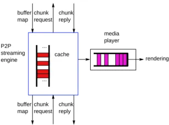
Figure 2 shows the software architecture of a peer in a mesh-pull system. The peer includes a P2P streaming engine and a media player. The streaming engine has the job of (i) retrieving chunks from partner peers and (possibly) from the origin server; (ii) storing the retrieved chunks in a cache; (iii) sharing media chunks stored in its cache with its partners; (iv) sending a copy (of the data) of each chunk it receives to the media player. As shown at the bottom of Figure 2, the peer sends a buffer map to each of its partner peers. The partner
original video server ... ... peer peer peer peer 1 2 2 new peer tracker server chunk chunk chunk chunk
Fig. 1. Mesh-pull P2P live streaming architecture
peer, having learned from the buffer map what chunks the peer has, issues requests for specific chunks. The peer then sends the requested chunks to the partner.
P2P streaming engine ... ... cache buffer map chunk request chunk reply buffer map chunk request chunk reply media player rendering
Fig. 2. A peer includes P2P streaming engine and media player. The
streaming engine trades chunks with partner peers.
A. Buffer Map and P2P Streaming Engine
The buffer maps (BMs) play a central role in our approach to infer system-wide quality. In this subsection, we describe the buffer map and P2P streaming engine in more detail. At any given instant, the P2P streaming engine caches up to a few minutes worth of chunks within a sliding window. Some of these chunks may be chunks that have been recently played; the remaining chunks are chunks scheduled to be played in the next few minutes. Peers download chunks from each other. To this end, peers send to each other buffer map messages; a buffer map message indicates which chunks a peer currently has buffered and can share. Specifically, the buffer map message includes the offset (the ID of the first chunk), the width of the buffer map, and a string of zeroes and ones indicating which chunks are available (starting with the chunk designated by the offset). Figure 3 illustrates the structure of a buffer map.
A peer can request a buffer map from any of its current partner peers. After peer A receives a buffer map from peer
offset 0 BM playable video gap 1 1 1 1 1 1 1 0 0 0 1 0 1 0 0 1 BM width time ... ...
Fig. 3. A peer’s buffer map, which indicates the chunks it currently has
cached
B, peer A can request one or more chunks that peer B has advertised in the buffer map. A peer may download chunks from tens of other peers simultaneously. The streaming engine continually searches for new partners from which it can download chunks. Different mesh-pull systems may differ significantly with their peer selection and chunk scheduling algorithms. The selection and scheduling algorithm used by CoolStreaming is documented in [1]. Peers can also download chunks from the origin server. The chunks are typically sent over TCP connections, although in some mesh-pull systems, video chunks are also transferred using UDP.
B. Media Player
When the client application is started, the media player is launched and the URL of the video stream is provided to the media player. From the client’s perspective, the server of the media content is the P2P streaming engine (which is in the same host as the media player). Once the media player is initialized, it sends (typically) an HTTP request to the P2P streaming engine. After having received the request, the P2P streaming engine assembles its chunks and header information into a media file and delivers of the file to the media player. Because new chunks continually arrive to the streaming engine, the streaming engine continually adds data to the file. Because some chunks may not arrive before the playout deadline, there may be “gaps” in the file. When the media player begins to receive the video from the streaming engine, it buffers the video before playback. When it has buffered a sufficient amount of continuous video content, it begins to render the video.
A video stream is commonly formated in one of four video formats: Window Media Video (WMV), Real Video (RMVB), Quicktime video or Macromedia Flash. For the sake of concreteness, let us consider mesh-pull P2P streaming systems that use WMV (as is often the case today). WMV videos use the Advanced Systems Format (ASF) [25]. An ASF file starts with a header object and is followed by a series of media data objects. The file header object includes various meta information for the file (i.e., the file identifier, buffering time and overall file bit-rate), number of available audio and video streams carried in the file, and meta information for each audio (i.e., sampling rate) and video stream (i.e., spatial resolution, compression algorithm). Each data object starts with an object header. The object header includes the sequence number of the object, the number of streams carried in the object, playback duration of the data object, and so on. In the payload of data objects, multiple media objects from different
streams (for example, a video and audio stream) may be carried and interleaved.
Because of the real-time nature of live streaming, each media chunk has a playback deadline (which can be different from one peer to another by a few minutes). When a chunk does not arrive before its playback deadline, the peer has two options: it can freeze the playback with the most recently displayed video frame and wait for the missing chunk to arrive; or it can skip the playback of the frames in the chunk and advance the deadlines for the subsequent chunks accordingly. The freeze is a natural consequence of the media playback when there are no video chunks in the buffer of the player. If there are still chunks available in the buffer of the player, the player continues playback even though those chunks might not be continuous; in this case, video playback skipping occurs. We have also observed that in many P2P live streaming systems, when the playback freezes for an extended period of time, the engine terminates the connection with the player and reinializes the entire streaming process; we refer to this impairment as rebooting.
III. HARVESTINGBUFFERMAPS
As described in Section II, peers in mesh-pull streaming systems exchange buffer maps among themselves. In this paper, we show how buffer maps can be used to infer many global-wide characteristics of of P2P live streaming systems. These characteristics include playback quality, time lags among users, and the video frame propagation pattern throughout the entire network. Our methodology has two
major steps: (i) continually harvest buffer maps from peers
scattered throughout the network;(ii)process (either in
real-time or off-line) the buffer maps to infer characteristics about global-wide system behavior. In this section we describe two approaches for harvesting buffer maps: active buffer-map crawling and buffer-map sniffing. We also describe how we specifically harvested buffer maps from the PPLive streaming system.
A. Buffer-Map Crawling
Buffer-map crawling is the process of remotely contacting a large number peers, and continually requesting and receiving buffer maps from these peers. To perform active buffer-map crawling, we need to accomplish the following tasks:
• Track the IP addresses (and port numbers) for the peers
in the system, accounting for peer churn. Tracking the peers is typically done by requesting lists of peers from the tracker and/or from the peers themselves [11].
• Using knowledge of the specific protocol of the P2P live
streaming system, send buffer-map request messages to the tracked peers.
• Receive buffer-map messages from the tracked peers and,
again using knowledge about the specific protocol, extract the actual buffer maps from the buffer-map messages. There are many challenges in building a buffer-map crawler. Most of the P2P mesh-pull live streaming systems are propri-etary. In order to establish partnerships with peers, generate
buffer map requests and interpret buffer map responses, it be-comes necessary to do an analysis of the proprietary protocol. If one is privy to the signaling protocol, then these tasks are relatively straightforward. Otherwise, this is typically done by collecting packets and analyzing them using one’s basic knowledge of how a mesh-pull P2P live streaming system operates. Second, a peer usually retrieves buffer maps by establishing a TCP connection from a remote peer; however, operating systems in general have constraints on the maximum rate to accept new TCP connections. When the remote peer has received a large number of TCP connection requests, there may not be a response to a buffer map request by the operating system. In addition, the peer application may not respond to buffer map requests when the application has already been overloaded with TCP connections. Utilizing TCP to probe the remote peers for buffer maps also incurs unavoidable overhead due to the establishment and termination of TCP connections. A single crawler may not be able to harvest quickly an accurate snapshot of buffer map distribution of peers in a popular channel.
B. Buffer-Map Sniffing
Recall that each peer participating in the system sends and receives buffer maps to and from other peers. We can therefore harvest buffer maps as follows:
• Connect several peer clients to the P2P live streaming
system.
• At each connected client, run a sniffer which grabs all
traffic sent and received by the client.
• Using knowledge about the specific knowledge about the
protocol, extract the buffer maps, along with the origin (IP addresses) of the buffer maps.
The sniffing nodes should be distributed globally throughout the network, in order to capture a diverse set of buffer maps. There is a tradeoff with respect to the number of sniffing nodes deployed. On one hand, we would like to have a large number of sniffers, which would increase the number of buffer maps collected. On the other hand, each sniffer node perturbs the system, as it downloads and redistributes chunks.
C. Harvesting Buffer-Maps in PPLive
PPLive is a typical mesh-pull P2P streaming system. PPLive
currently provides 300+ channels. The bit rates of video
programs mainly range from 300 kbps to 500 kbps. PPLive
does not own video content; the video content is mostly feeds from TV channels, TV series and movies in Mandarin. The channels are encoded in two video formats: Window Media Video (WMV) or Real Video (RMVB). The encoded video content is divided into chunks and distributed to users through the PPLive P2P network. PPLive is described in some detail in [12].
It is challenging to conduct measurement studies over PPLive because the PPLive protocol is proprietary. In partic-ular, in order to build the buffer map harvesting tools that are used in this paper, we had to analyze the PPLive protocol using packet traces from passive sniffing. With these efforts, we
were able to understand critical portions of PPLive’s signaling protocols.
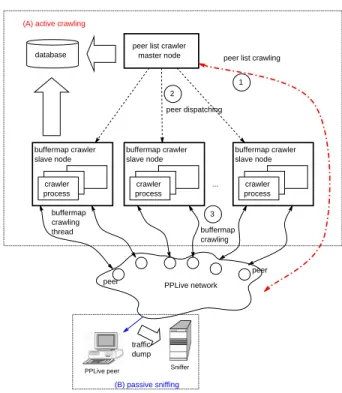
Our PPLive buffer-map crawler utilizes both UDP and TCP transport for collecting peer lists, and TCP for collecting buffer maps from many remote peers during the same period of time. Figure 4 shows the architecture of our PPLive buffer-map crawler. Recall from Section II that each peer watching a particular channel maintains a peer list, which lists other peers currently watching the same channel. In PPLive, any peer A can send to any other peer B, within a UDP datagram or a TCP segment, a request for peer B’s peer list. The crawler sweeps across the peers watching the channel and obtains the peer list from each visited peer. Given the IP addresses of the remote peers on the peer list, we augmented the crawler with a TCP component that retrieves the buffer map from these remote peers. To this end, as we crawl each peer, the crawler sends a request for the peer’s buffer map. We then parse the buffer maps off-line, to glean information about buffer resources and timing issues at the remote peers throughout the network.
In general, operating systems have a maximum TCP thread constraint that one host is able to maintain. To trace a large set of the peers, we deploy a master-slave crawling architecture to harvest buffer maps through the network. As shown in Figure 4, in step 1, the peer list crawler tracks the peers of one channel in the PPLive network. This peer list crawler serves as a buffer map crawling master. At the same time, we initiated multiple buffer map crawling slaves. The buffer map master assigns 30 peers to each slave. Each slave then probes these 30 peers to harvest their buffer maps.
While running the crawler, we utilize WinDump [26] to passively sniff from three PPLive control nodes: one in New York City with residential cable-modem access; one in New York City with university Ethernet access; and one in Hong Kong with university Ethernet access. The buffer maps are embedded in the application data in these captured traffic traces. Given the knowledge of the PPLive signaling protocol, we are able to extract the buffer maps from these traces for our analysis. A summary of the buffer data collected (from the crawler and sniffers combined) is given in Table I.
IV. INFERRING PLAYBACK QUALITY FROM BUFFER MAPS
In the previous section, we showed how buffer maps can be harvested from a P2P live streaming system. In this section, we show that the buffer maps can be used to infer important characteristics of the performance of the P2P live streaming system, including playback continuity and start-up latency. A. Automatic Playback Continuity Evaluation
In order to study the relationship between buffer-map values and playback continuity, it is desirable to have a mechanism that can automatically evaluate the playback continuity of a video stream received at a media player. To this end, we developed a stream analyzer to capture the arrival process of the media objects to the media player from the streaming engine, and estimate the user perceived quality. Our analyzer tracks the sequence numbers of the arriving media objects and the presentation time of the latest media object, from which
peer list crawler master node PPLive network buffermap crawler slave node crawler process buffermap crawler slave node crawler process buffermap crawler slave node crawler process ... database buffermap crawling thread peer dispatching 1 2
peer list crawling
buffermap crawling
3
PPLive peer Sniffer
traffic dump (A) active crawling
(B) passive sniffing
peer
peer
Fig. 4. Peer buffer map harvesting
we estimate the playback impairments including freezing and rebooting. We now describe how we estimate when playback freezing occurs
Typically, a media file consists of two streams, video and audio stream. We use the video stream for illustration. A video stream consists of a sequence of video objects. Each video
object is identified by an increasing sequence numberi (i=
1,2, . . .). Let ti be the relative presentation time of the i-th object, which is obtained from the video object header. Let
ai be the arrival time, which is recorded when our analyzer
receives this object. Letτbe the initial playback pre-buffering
delay, which is specified in the streaming engine. Let bi and
fi be the actual playback starting time and finishing time,
respectively.
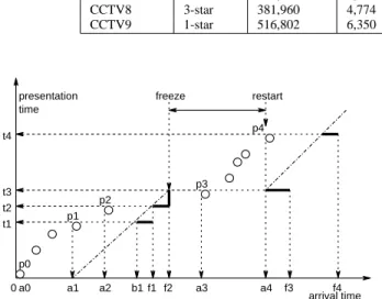
The presentation time stamped on the video objects can be used to estimate when video freezing occurs. Figure 5 depicts how we estimate video freeze and resume when all
video objects arrive in order. After the video objectp2finishes
playback at time f2, there are no video objects in the buffer
(f2< a3); hence, our analyzer declares that playback freezes
at timef2. During the playback freezing period, the analyzer
continues receiving video objects from the streaming engine.
The video object p3 arrives at time a3. The analyzer starts
to buffer video objects without playback. When it receives sufficient video objects, the time duration of the buffered
objects(t4−t3)is larger than the pre-buffering threshold τ
and the playback restarts. Hence, the analyzer estimates the
video freezing period isa4−f2.
We have just described how our analyzer estimates when freezing occurs and the duration of the freezing for the case when all video objects arrive in order. Our analyzer also handles the case when objects arrive out of order, and also estimates when rebooting occurs. We have validated the
ana-TABLE I
SUMMARY OF HARVESTED BUFFER MAPS
channel name popularity bit rate (bps) chunk size (byte) buffer maps total peers duration (minutes)
CCTVNews 5-star 381,960 4,774 1,952,837 8,120 635 CCTV1 4-star 381,960 4,774 1,440,117 6,668 636 CCTV3 4-star 381,960 4,774 1,789,331 12,392 650 CCTV8 3-star 381,960 4,774 1,359,236 6,985 751 CCTV9 1-star 516,802 6,350 1,263,097 2,125 1,031 0 arrival time presentation time p1 p0 f1 p2 a2 a1 p3 f2 a3 p4 a4 f3 f4 freeze restart a0 b1 t1 t2 t3 t4
Fig. 5. Playback time diagram with video freezing
lyzer by physically watching PPLive channels and observing the analyzer indicates that impairments actually occur.
B. Correlation between buffer maps and video continuity In this section, we demonstrate there exists a correlation between the buffer map values and the playback impairment events as determined by our analyzer. Because of this cor-relation, we will be able to quantify network-wide playback quality from the harvested buffer maps in Section V and VI.
We performed a number of experiments, and in each of these experiments such a correlation was exhibited. In this section we provide an illustrative example experiment. In this experiment, we connected a campus peer to a popular, four-star PPLive channel (CCTV1) for a three-hour period. During this three-hour period, the number of peers viewing the channel increased from about 1000 to about 2800, as shown in Figure 6. (These values were obtained from our peer-list crawler.) During this time, the output of the PPLive streaming engine was fed into our streaming analyzer. Also during this time, we captured the buffer maps that were sent from this monitored campus peer to its partner peers.
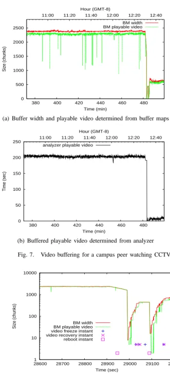
In Figure 7(a), we plot the Buffer Map (BM) width and the BM playable video, which are obtained from the captured buffer maps. As shown in Figure 3, the BM width is the difference between the newest and oldest chunk number ad-vertised in a buffer map message. The BM playable video is the number of contiguous chunks in the buffer map, beginning from the offset. We also plot the analyzer playable video (in seconds) as determined by our stream analyzer in Figure 7(b). It is important to note that the BM playable video, as determined from the buffer maps, and the analyzer playable video, as determined from the stream analyzer, will not be equal because the actual playback point is somewhere in the
800 1000 1200 1400 1600 1800 2000 2200 2400 2600 2800 380 400 420 440 460 480 11:00 11:25 11:50 12:15 12:40 # of peers Time (min) Hour (GMT-8) total peers
Fig. 6. Peer evolution in trace for CCTV1
middle of the BM playable video.
We observe that the shape of the BM playable video curve, obtained from the buffer maps, is very similar to the analyzer playable video, obtained from the analyzer. Note in particular that both curves show a brief period of no buffered video in
the vicinity oft= 481minutes.
In Figure 8 we zoom in on the buffer map evolution and also plot the time instants of the playback impairment events reported by the analyzer, including two streaming reboots and four playback freezes. We observe that playback impairments indeed occur only when the BM playable video, determined from the buffer maps, becomes very small. Hence, we intro-duce the following heuristic to detect freezing events: Given a
sequence of buffer maps for one peer, record the time instantt1
of the first buffer map when the BM playable video is less than 5 chunks. We then continue to track the BM playable video of consecutive subsequent buffer maps. If the BM playable video remains less than 5 chunks for 4 seconds, we say a freezing
event occurs att1. A freeze event ends when the BM playable
video is larger than the pre-buffering time of the stream. In addition to the playable video size, the offset value in the buffer map can be used to infer playback continuity. Under normal circumstances, the buffer map offset should increase at a constant rate: if this rate varies significantly, PPLive reboot occurs. Figure 9 shows the buffer map offset rate of this campus peer. For this video trace CCTV1, the media playback bit rate is 381 kbps; the buffer map offset normally increases
at r = 10 blocks/sec = 4774·8·10 kbps = 381 kbps. We
see that when there is a sudden increase in the offset rate, a reboot occurs (which also explains the first reboot occurrence in Figure 8). We use the following heuristic to detect reboot events: compute the average rate at which the offset increases over 40 seconds. If this average rate is 10% higher than the
0 500 1000 1500 2000 2500 380 400 420 440 460 480 11:00 11:20 11:40 12:00 12:20 12:40 Size (chunks) Time (min) Hour (GMT-8) BM width BM playable video
(a) Buffer width and playable video determined from buffer maps
0 50 100 150 200 250 380 400 420 440 460 480 11:00 11:20 11:40 12:00 12:20 12:40 Time (sec) Time (min) Hour (GMT-8)
analyzer playable video
(b) Buffered playable video determined from analyzer
Fig. 7. Video buffering for a campus peer watching CCTV1
1 10 100 1000 10000 28600 28700 28800 28900 29000 29100 29200 Size (chunks) Time (sec) BM width BM playable video video freeze instant video recovery instant reboot instant
Fig. 8. Playback impairments of a campus peer in trace CCTV1.
nominal playback rate or it is less than 90% of the nominal playback rate, the potential reboot alarm is issued. If in 3 consecutive offset rate checking rounds, which lasts over 120 seconds, all three reboot alarms are issued, we say a playback reboot occurs. Otherwise, the reboot alarm is cleared.
We conclude that the playback freezing is closely correlated with the size of the BM playable video as determined from the buffer maps. In Figure 8, when this playable video is smaller than some threshold (e.g., 5 blocks) and stays in this state for a few seconds, playback freezing occurs.
C. Correlation between buffer maps and start-up latency Buffer maps can also be used to infer the start-up latency of peers. As shown in Figure 10, in PPLive, when a peer joins the
1 10 100
28600 28800 29000 29200 29400
Increasing rate (chunk/sec)
Time (sec)
increasing rate of buffer map offset reboot instant reported by the analyzer
Fig. 9. The rate of the buffer map offset of a campus peer in trace CCTV1.
network and has no chunks in its engine buffer, it sends buffer maps with playback offset equal to zero and a buffer size equal to zero. After a peer obtains chunks from other peers, the offset is set to a non-zero value. The streaming engine will start the player when the size of the cached playable video size exceeds a specified pre-buffering video threshold. This threshold is a system parameter of the streaming engine, which an end user may configure in the option settings of the application. The consecutive buffer maps provide snapshots of the video chunks in the buffer. Therefore, we can infer the start-up time of the playback of a peer given the sequence of the buffer maps of this peer with the first buffer map having a zero-valued offset. In this example, the pre-buffering video size is 5 seconds in time (roughly 50 chunks); hence, the startup time is roughly 17 seconds. 1 10 100 1000 130 140 150 160 170 180 190 200 Size (chunks) Time (sec) 50 chunks
offset zero startup
latency BM width BM playable video
Fig. 10. Buffer map evolution at start-up of a campus peer in trace CCTV1.
V. NETWORK-WIDE SERVICEQUALITY
Using the methodologies described in the previous section, we can infer video playback quality on remote peers that we cannot monitor directly. In this section, we report network-wide service quality results for PPLive. We present results for several important quality metrics: playback continuity, including freezes and reboots, start-up latency and time lags among peers.
A. Playback Continuity
The most important measure of service quality of a stream-ing system is the continuity of video playback at the user
hosts. Using the tools described in Section IV-B, we harvested the five sets of buffer maps shown in Table I. We then processed the buffer maps using the heuristic described in Section IV. Table II reports playback continuity, freezes and
reboots, experienced by randomly sampled peers during 10
one-hour periods. For each one-hour period, we select peers with at least 50 captured buffer maps. Among the sampled peers, we count the number of the reboot/freeze peers that have at least 1 playback reboot/freeze event in this one-hour period. The reboot/freeze peer ratio is defined as the ratio between the reboot/freeze peer and the total number of sampled peers in this one-hour period.
From Table II, we observe that the peers in the monitored channels have smooth video playback most of the time. For
channel CCTV3 and CCTV8, more than 90% peers never
experienced any freezes or reboots within one hour time periods. For channel CCTVNews and CCTV1, the freeze peer ratio and reboot peer ratio varies over time. The general trend is that the more peers in the system, the lower the freeze and reboot ratio. Compared with the other four channels, channel CCTV9 has relatively high freeze and reboot ratio over the ten hours period. Looking at the number of peers, we found the number of peers in this channel is much lower than in the other four channels.
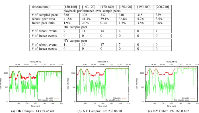
To get more details on playback impairments, we zoom in to one time period, from 2.5 hours to 3.5 hours, when a high ratio of peers in channel CCTVNews experience freezes and reboots. Table III lists the freeze and reboot ratios among all sample peers and the number of playback impairments on two
specific peers every 10 minutes. We see a high reboot ratio
among sample peers and two specific peers experienced lots
of reboots every10minutes.
To understand the causes of the frequently occurring play-back impairments, we plot in Figure 11 the BM playable video
on three. Before t = 182 minutes, all three peers have a
small and highly variable amount of BM playable video in
their buffers. After t = 182 minutes, the playable video in
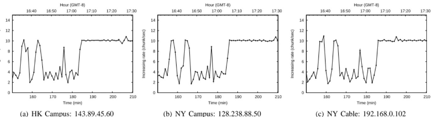
all three peers stays at a high level. We further look into the rate at which buffer map offsets increase for the three peers during that time period. Since the playback time for a chunk
is 0.1 seconds, to maintain steady playback, the buffer map
offset should increase at a rate of10chunks per second. From
Figure 12, we observe that before t = 182, the three peers
cannot advance their buffer map offset at the playback rate of
10chunks/sec. They experience severe playback impairments.
Aftert= 182, the rate of increase of buffer map offset reaches
the playback rate for all three peers. Based on the strong correlation of playback impairments on three peers, we infer that this is a network-wide quality degradation. One important factor affecting network-wide service quality is the number of peers in the network. The more peers in the network, the more stable the network-wide service quality. We suspect the
frequent playback impairments beforet= 182is because the
number of peers in that time range is not large enough. To test this, we plot in Figure 13 the evolution of peer population
from time 0 to 210 minutes. The number of peers before
t = 180 minutes oscillates around 700. For some reason,
starting from t= 180minutes, more and more peers join the
600 700 800 900 1000 1100 1200 1300 1400 1500 160 170 180 190 200 210 16:40 16:50 17:00 17:10 17:20 17:30 # of peers Time (min) Hour (GMT-8)
Fig. 13. Evolution of the Number of Peers in CCTVNews
channel and the peer number keeps increasing until the end of the observation window. This verifies our conjecture that peer population largely affects network-wide service quality.
B. Start-up Latency
The very first quality measure that a user perceives after joining a channel is the start-up latency. We use the heuristic described in Section IV-C to estimate a peer’s start-up delay from its buffer maps. The total number of peers whose start-up
processes were captured in trace CCTV9 is220. For each peer,
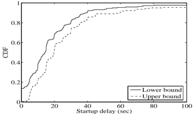
we estimated the upper bound and lower bound of its start-up delay. We plot in Figure 14 the probability distribution of the lower and upper bounds for peers in that channel. Table IV presents the start-up delays for peers in five different
0 20 40 60 80 100 0 0.2 0.4 0.6 0.8 1
Startup delay (sec)
CDF
Lower bound Upper bound
Fig. 14. The Distribution of Start-up Latencies on Peers in trace CCTV9
channels. For each channel, we report the median values of the lower bound and upper bounds of peers in that channel. The variance of the startup delay is not significantly. For example, for CCTV9, the standard deviation (STD) of the lower bound of the startup delay is 41.7 seconds and the STD of the upper bound is 51.3 seconds.
C. Playback Lags among Peers
In a mesh-pull P2P streaming system, the progress of video playback on a peer is determined by how fast it collects video chunks from the system. The variations in chunk retrieval times from peer to peer introduce time lags among the peers.
TABLE II
PLAYBACK IMPAIRMENTS ON PEERS OF FIVE CHANNELS WITHIN TEN HOURS
time(hour) [0,1] [1,2] [2,3] [3,4] [4,5] [5,6] [6,7] [7,8] [8,9] [9,10]
channel CCTVNews
# of sampled peers 1206 950 868 973 1230 1414 1253 1054 974 827
reboot peer ratio 18.8% 38.5% 41.9% 14.1% 3.4% 2.2% 2.6% 3% 4.4% 4.1%
freeze peer ratio 1.8% 3.1% 2.9% 2.0% 1% 0.6% 0.7% 0.9% 2.7% 3.1%
channel CCTV1
# of sampled peers 301 382 605 1107 1104 926 714 1038 1438 1141
reboot peer ratio 20% 15% 4.8% 2.1% 1.4% 3.6% 1.7% 2.2% 2.4% 1.3%
freeze peer ratio 9.0% 9.0% 2.5% 0.6% 0.8% 2.1% 0.6% 0.8% 1.3% 1%
channel CCTV3
# of sampled peers 899 920 996 956 1413 2141 2835 2307 1848 1215
reboot peer ratio 7.6% 6.6% 7.3% 5% 2.8% 7.9% 10.7% 9.5% 8.6% 14.4%
freeze peer ratio 1.1% 1.7% 2.2% 1.4% 0.9% 2% 4.3% 4.2% 2.3% 3.1%
channel CCTV8
# of sampled peers 435 393 564 667 860 1188 1313 1426 1085 974
reboot peer ratio 3% 5.1% 3.7% 4.2% 2.7% 2% 0.7% 0.5% 1.2% 1%
freeze peer ratio 1.4% 1% 1.2% 1.4% 0.9% 1.2% 0.7% 0.4% 0.2% 0.3%
channel CCTV9
# of sampled peers 207 173 160 184 199 247 340 397 353 311
reboot peer ratio 26.6% 44.5% 38.1% 35.3% 32.2% 40.1% 29.7% 26.2% 15.9% 16.7%
freeze peer ratio 4.4% 20.2% 23.1% 20.7% 12.1% 14.6% 12.7% 6.8% 9.6% 5.5%
TABLE III
PLAYBACK IMPAIRMENTS ON PEERS OF ONE CHANNEL WITHIN ONE HOUR
time(minute) [150,160] [160,170] [170,180] [180,190] [190,200] [200,210]
playback performance over sample peers
# of sampled peers 320 305 332 310 315 339
reboot peer ratio 41.8% 41.3% 39.1% 36.8% 5.7% 3.5%
freeze peer ratio 1.9% 2.0% 0.3% 1.3% 3.8% 0.6%
HK campus peer # of reboot events 9 11 14 4 0 4 # of freeze events 0 0 0 0 0 0 NY campus peer # of reboot events 11 10 17 7 0 0 # of freeze events 0 0 0 0 0 0 10 100 1000 160 170 180 190 200 210 16:40 16:50 17:00 17:10 17:20 17:30 Size (chunks) Time (min) Hour (GMT-8) BM width BM playable video (a) HK Campus: 143.89.45.60 10 100 1000 160 170 180 190 200 210 16:40 16:50 17:00 17:10 17:20 17:30 Size (chunks) Time (min) Hour (GMT-8) BM width BM playable video (b) NY Campus: 128.238.88.50 10 100 1000 160 170 180 190 200 210 16:40 16:50 17:00 17:10 17:20 17:30 Size (chunks) Time (min) Hour (GMT-8) BM width BM playable video (c) NY Cable: 192.168.0.102
Fig. 11. Correlation on BM playable video of three peers in trace CCTVNews
1) Maximum Time Lags: One measure of peer playback synchronization is the time lags between the “fastest” and the “slowest” peer. To obtain maximum time lags, we merge buffer map traces collected by three monitors and group buffer maps into time bins of 5 seconds. For each bin, we calculate the difference between the maximum and the minimum offset of the buffer maps in that bin. The difference indicates the maximum playback lag among the peers monitored in that time slot. Figure 15 shows that the maximum time lags among peers
monitored by the three peers fluctuate around 150 seconds
within a one hour time period.
2) Tiering Effect: Other than the maximum time lags, we also want to explore the structure embedded in the delay performance of peers in a mesh-pull P2P streaming system. In a tree-based video streaming system, a user’s playback delay is determined by its distance to the server. When grouped into tiers according to their distances, users in a tier close to the source will consistently have smaller playback time
0 2 4 6 8 10 12 14 160 170 180 190 200 210 16:40 16:50 17:00 17:10 17:20 17:30
Increasing rate (chunk/sec)
Time (min) Hour (GMT-8) (a) HK Campus: 143.89.45.60 0 2 4 6 8 10 12 14 160 170 180 190 200 210 16:40 16:50 17:00 17:10 17:20 17:30
Increasing rate (chunk/sec)
Time (min) Hour (GMT-8) (b) NY Campus: 128.238.88.50 0 2 4 6 8 10 12 14 160 170 180 190 200 210 16:40 16:50 17:00 17:10 17:20 17:30
Increasing rate (chunk/sec)
Time (min) Hour (GMT-8)
(c) NY Cable: 192.168.0.102
Fig. 12. Correlation on buffer map offset increase rates of three peers in Trace CCTVNews
TABLE IV
MEDIAN OFSTARTUPLATENCIES
Trace Captured Peers Lower bound Upper bound
(sec) (sec) CCTVNews 38 11.8 17.5 CCTV1 74 13.3 19.8 CCTV3 1405 50.3 94.9 CCTV8 92 5.98 12.8 CCTV9 220 14.2 19.7 0 50 100 150 200 250 300 12000 12500 13000 13500 14000 14500 15000 15500 Time (sec) Time (sec)
Fig. 15. Maximum time lags among peers in trace CCTVNews
delays than users in a tier farther away. In a mesh-pull P2P streaming system, to deal with peer churn, there is no fixed tree structure. Peering links are established/removed dynamically. Consequently, unlike in a tree-based system, the regularity in the relative delay performance among peers cannot be assumed. On the other hand, in a mesh-pull based system, the peering links are not purely random. They are driven by peer visibility and chunk availability, which are largely determined by the peers’ network connections and their locations in the streaming system. With this in mind, one can expect some structure in peering topology, and peer delay performance in turn. In this section, by examining buffer map traces collected from peers with different geographical locations and different network access, we present results demonstrating a tiering effect in the playback time lags.
To expose the ordering of the playback delays on different peers, we infer the playback progress of a remote peer by checking the offsets of buffer maps collected from that peer. We define the relative playback difference between two peers as the offset difference of these two peers. More specifically,
suppose that we obtained one buffer map of peer 1 att1 with
the buffer map offset∆1, and one buffer map of peer 2 att2
with the offset∆2. The playback difference is computed as
δ=(∆2−∆1)∗L
r −(t2−t1),
whereL denotes the chunk size and r denotes the playback
bit rate.
We use three different traces taken at the same time to explore the tiering effect. For each trace, using the local playback time on the monitor as the reference point, we
calculate the relative playback differences for the6peers from
which we collected the most buffer maps. We plot in Figure 16 the evolution of the relative playback differences over a one hour time period. We observe that there exists a clear ordering among peers’ playback lags in all three traces. In addition, the relative playback differences are quite stable over the one-hour time period. From the playback lags between two peers, one can also infer the direction of video data flow between them. It is very unlikely for a peer to download video from a peer whose playback time is tens of seconds behind.
For the trace collected from the Hong Kong campus peer, Figure 16(a) shows that only one peer out of the six peers is ahead of the local peer. We conjecture that the Hong Kong campus is close to the video source server. It can download video chunks quickly from the server and redistribute them to other peers in Hong Kong or places farther away exploiting its high upload capacity. In Figure 16(b), for the trace collected from the campus peer in New York, about half of its peers are ahead of it and the other half are behind it. We conjecture that this peer downloads video chunks from peers in Asia and acts as a proxy to upload video chunks to peers in the US. Although in the same city as the New York campus peer, the cable peer in New York has very different delay performance relative to its peers. Figure 16(c) shows that most of its peers are ahead. We conjecture that this residential peer uploads little traffic to its peers. We also calculate the relative playback delay among the three monitors. The Hong Kong campus peer’s local
playback time is around 80 seconds ahead of the New York
campus peer; the New York residential peer’s local playback
time is 20 seconds behind the New York campus peer. This
suggests that both the location and network access of a peer largely affect its playback delay.
-120 -100 -80 -60 -40 -20 0 20 40 12000 12500 13000 13500 14000 14500 15000 15500 Time (sec) Time (sec) (a) HK Campus: 143.89.45.60 -20 0 20 40 60 80 100 12000 12500 13000 13500 14000 14500 15000 15500 Time (sec) Time (sec) (b) NY Campus: 128.238.88.50 -40 -20 0 20 40 60 80 100 12000 12500 13000 13500 14000 14500 15000 15500 Time (sec) Time (sec) (c) NY Cable: 192.168.0.102
Fig. 16. Tiering effect in trace CCTVNews: peers have a stable relative order on their playback lags.
VI. VIDEOOBJECTPROPAGATION
Buffer maps collected from peers in the same P2P streaming network not only reflect network-wide video playback quality but also provide valuable information for inferring how video chunks propagate among peers inside the network.
Chunk propagation in a P2P streaming system is governed by peering strategies and chunk scheduling schemes on all peers. Without sniffing traffic on all peers, we cannot trace the detailed propagation of a chunk among all peers. However, we can utilize harvested buffer maps to infer when a chunk is downloaded by a monitored peer. Based on that, we obtain a sampled view of the availability of a chunk among all peers in the system. After a chunk is generated by the server, it will be downloaded by peers. After a peer successfully downloads the chunk, the peer will make it available for other peers for download until that chunk falls outside its buffer map window. How long a chunk is available in the system and how many peers can upload that chunk at a given time can be inferred from the buffer maps.
A. Chunk Life Time
We first look at chunk life time. The life time of a chunk is defined as the duration from the first appearance of that chunk in the collected buffer maps to the last time of its appearance. Chunk life time tells us for how long a chunk is available for download in the network. Since we only collect buffer maps from a subset of peers, the reported chunk life time is an under-estimate of the real chunk life time. In Figure 17(a), a chunk
stays in one peer’s buffer for about210seconds; however, this
chunk may still be available in some other peers’ buffer. We
observe that the chunk life time in the network is about 250
seconds. This peer life CDF curve is computed by tracing the chunk life on the NY campus peer.
B. Evolution of Chunk Availability
We define the availability of a chunk at a given time as the fraction of peers that make that chunk available for other peers to download. The higher the chunk availability the higher the upload supply and the lower the download demand for that chunk. Figure 18 shows availability snapshots for a range of chunks among randomly sampled peers in two channels. In Figure 18(a), we tracked 4500 consecutive chunks among the
sampled 122 peers. The tracking results are reported every 90 seconds. We observe that the chunk availability percentage can
reach as high as80%. For a given snapshot, a wide window
of chunks for 150 seconds have availability above70%. Also
the position of the window shifts at a steady rate from one snapshot to another snapshot. Shown in Figure 18(b), in the 1-star channel CCTV9, the chunk availability percentage is much smaller than the popular CCTVNews. For a given snapshot, chunks falling in the window only have availability around
40%. Peers in CCTV9 have difficulty to locate chunks and the
playback is thus susceptible for various service impairments.
C. Evolution of Chunk Retrieval Ratio
The playback quality on a peer is largely determined by whether the peer can retrieve video chunks before their playback deadlines. Using buffer maps, for a specific chunk, we can calculate the fraction of peers that have retrieved the chunk at any time instant. The chunk retrieval ratio among
peers should grow over time until it reaches close to 1.
The speed of the growth is a good measure of P2P video distribution efficiency. Figure 19 shows the retrieval ratios of five chunks from 122 randomly sampled peers in two channels: CCTVNews with a 5-star popularity and CCTV9 with a 1-star popularity. The five chunks are chosen such that two adjacent
chunks have presentation time difference of 10 seconds. All
chunk retrieval ratios evolve in a similar pattern. They increase
quickly to about65%within 20 seconds. The increase trend
slows down after the knee point until it converges to around
95%. However, as illustrated in Figure 19(b), in the less
popular channel CCTV9, the knee points come earlier, at
around 30%. The chunk retrieval ratios converge in a wider
range from50%to75%. This suggests that chunk propagation
in a small P2P streaming system is slower and more variable than in a large system. One direct consequence is that less popular channels have worse quality.
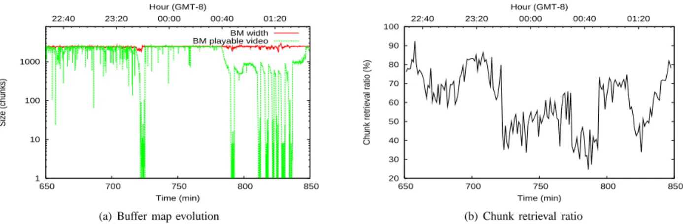
To see the impact of chunk retrieval ratio on individual peer’s playback quality, we plot in Figure 20(a) the evolution of buffer sizes on the Hong Kong campus sniffer. Figure 20(b) shows the chunk retrieval ratio among its peers during the same time period. Whenever the sniffer has low video buffer
200 250 300 0 0.2 0.4 0.6 0.8 1 Time (sec)
CDF
Peer life Network life (a) CCTVNews 1500 200 250 300 0.2 0.4 0.6 0.8 1 Time (sec)CDF
Peer life Network life (b) CCTV9Fig. 17. Distribution of chunk lifetime in two channels
0 10 20 30 40 50 60 70 80 90 0 500 1000 1500 2000 2500 3000 3500 4000 4500
Chunk availability percentage (%)
Chunk ID t0 t0+90sec t0+180sec t0+270sec (a) CCTVNews 0 10 20 30 40 50 60 70 80 0 500 1000 1500 2000 2500 3000 3500 4000 4500
Chunk availability percentage (%)
Chunk ID t0 t0+90sec t0+180sec t0+270sec (b) CCTV9
Fig. 18. Chunk availabilities among peers at four time snapshots
0 10 20 30 40 50 60 70 80 90 100 16050 16100 16150 16200
Chunk retrieval ratio (%)
Time (sec) chunk 1 chunk 2 chunk 3 chunk 4 chunk 5 (a) CCTVNews 0 10 20 30 40 50 60 70 80 12300 12350 12400 12450 12500 12550 12600
Chunk retrieval ratio (%)
Time (sec) chunk 1 chunk 2 chunk 3 chunk 4 chunk 5 (b) CCTV9
Fig. 19. Evolutions of chunk retrieval ratios for five sampled chunks
VII. CONCLUSION
Based on remotely gathering buffer maps, we have devel-oped a methodology to estimate network-wide quality in mesh-based P2P live streaming systems. A peer’s buffer map pro-vides a light-weight snapshot of chunk availability at that peer. We have shown that quality can be inferred from buffer maps. We illustrated this methodology by applying it to a specific P2P live streaming system, namely, PPLive. The methodology enabled us to estimate several important network-wide quality
measures, including network-wide viewing continuity, startup latency, and peer lags. It also enabled us to track the propa-gation on chunks throughout the P2P network. As discussed in the Introduction, this methodology can be used by service providers, by third parties who monitor performance on behalf of customers and advertisers, and by researchers who seek a deeper understanding of the behavior of mesh-pull P2P live streaming systems.
1 10 100 1000 650 700 750 800 850 22:40 23:20 00:00 00:40 01:20 Size (chunks) Time (min) Hour (GMT-8) BM width BM playable video
(a) Buffer map evolution
20 30 40 50 60 70 80 90 100 650 700 750 800 850 22:40 23:20 00:00 00:40 01:20
Chunk retrieval ratio (%)
Time (min) Hour (GMT-8)
(b) Chunk retrieval ratio
Fig. 20. Correlations between the playback quality of a monitored peer and the chunk retrieval ratio in the whole network
A. Acknowledgements
We thank Jian Liang and Chao Liang for their help in the early stages of this research.
REFERENCES
[1] X. Zhang, J. Liu, B. Li, and T.-S. P. Yum, “DONet/CoolStreaming: A Data-driven Overlay Network for Peer-to-Peer Live Media Streaming,”
IEEE INFOCOM, vol. 3, Mar. 2005, pp. 2102 – 2111.
[2] “PPLive,” http://www.pplive.com. [3] “PPStream,” http://www.ppstream.com. [4] “UUSee,” http://www.uusee.com/. [5] “SopCast,” http://www.sopcast.org/. [6] “Boiling point TV,” http://tv.net9.org/. [7] “VVSky,” http://www.vvsky.com.cn. [8] “TVAnts,” http://www.tvants.com. [9] “QQLive,” http://tv.qq.com/. [10] “Tvkoo,” http://www.tvkoo.com/.
[11] X. Hei, C. Liang, J. Liang, Y. Liu, and K. W. Ross, “Insights into PPLive: A measurement study of a large-scale P2P IPTV system,” IPTV
workshop in conjunction with WWW2006, May 2006.
[12] ——, “A measurement study of a large-scale P2P IPTV system,” IEEE
Transactions on Multimedia, Oct. 2007, to appear.
[13] S. Ali, A. Mathur, and H. Zhang, “Measurement of commercial peer-to-peer live video streaming,” First Workshop on Recent Advances in
Peer-to-Peer Streaming, Aug. 2006.
[14] M. Pinson and S. Wolf, “A new standardized method for objectively measuring video quality,” IEEE Transactions on Broadcasting, vol. 50, no. 3, pp. 312 – 322, Sep. 2004.
[15] D. Loguinov and H. Radha, “Large-scale experimental study of Internet performance using video traffic,” SIGCOMM Comput. Commun. Rev., vol. 32, no. 1, pp. 7–19, 2002.
[16] S. Winkler and R. Campos, “Video quality evaluation for Internet streaming applications,” Proc. SPIE, vol. 5007, June 2003, pp. 104–115. [17] A. Reibman, S. Sen, and J. V. der Merwe, “Video quality estimation for
Internet streaming,” WWW ’05, 2005, pp. 1168–1169.
[18] A. Reibman, S. Sen, and J. Van der Merwe, “Analyzing the spatial quality of Internet streaming video,” Workshop on Video Processing and
Quality Metrics for Consumer Electronics (VPQM), Jan. 2005.
[19] ——, “Network monitoring for video quality over IP,” Picture Coding
Symposium, Dec. 2004.
[20] S. Tao, J. Apostolopoulos, and R. Guerin, “Real-time monitoring of video quality in IP networks,” NOSSDAV ’05, 2005.
[21] T. Silverston and O. Fourmaux, “P2P IPTV measurement: A comparison study,” University Paris 6 LIP6/NPA Laboratory, Tech. Rep., Oct. 2006. [22] L. Vu, I. Gupta, J. Liang, and K. Nahrstedt, “Mapping the PPLive network: Studying the impacts of media streaming on P2P overlays,” Department of Computer Science, University of Illinois at Urbana-Champaign, Tech. Rep. UIUCDCS-R-2006-275, Aug. 2006.
[23] B. Cohen, “Incentives Build Robustness in BitTorrent,” P2P-Econ, June 2003.
[24] “BitTorrent,” http://bittorrent.com/.
[25] “Advanced systems format (ASF) specification,” 2004. [26] “Windump,” http://www.winpcap.org/windump/.