Scheduling Intermediate Storage Multipurpose
Batch Plants Using the S-Graph
Javier Romero and Luis Puigjaner
Chemical Engineering Dept., Universidad Polite`cnica de Catalunya, E-08028 Barcelona, Spain
Tibor Holczinger and Ferenc Friedler
Dept. of Computer Science, University of Veszpre´m, Egyetem u. 10, H-8200, Veszpre´m, Hungary
A graph theoretical approach is proposed for the optimal scheduling of multipurpose batch plants when constraints on intermediate storage allocation are met. The novel S-graph representation is extended and combined with a set of rationales to consider intermediate storage policy in production scheduling. This set of rationales accelerates the optimization procedure, reducing the searching tree from the very beginning, without losing optimality. It is assumed that the storage units can be commonly used throughout the plant to achieve maximum plant flexibility. Therefore, the problem solved suggests the more general batch-process transfer strategy, common intermediate storage policy (CIS). This policy is suggested for more flexible use of intermediate storage units. The accuracy of this proposed algorithm is tested with an exhaustive B&B search algorithm. The methodology is compared with other CIS algorithms and is applied to solve several case studies. The benefits of considering this kind of storage coupled with the use of the proposed algorithm are discussed through motivating examples.© 2004 American Institute of Chemical EngineersAIChE J,50: 403– 417, 2004
Keywords: scheduling, schedule-graph, intermediate storage, CIS, FIS
Introduction
Because of the staged nature of process equipment in batch chemical plants, intermediate storage appears to be a vital component for unblocking batch processes. Storage installed between processing stages can help reduce idle times in these stages by freeing them to process other batches and thus increase equipment utilization and productivity of multiprod-uct/multipurpose batch processes (Ku and Karimi, 1988). In addition, intermediate storage constitutes an important compo-nent in mitigating the material flow imbalance of feedstock materials and intermediate products in order to meet finished-product demand. However, increasing the storage facility is penalized by a larger investment, a reduction in available
space, and the associated environmental issues because of more cleanings, among other considerations. Hence, efficient man-agement of storage facilities at the production scheduling stage is necessary to improve at most performance of batch processes using these facilities.
The rules governing the transfer of batches between process-ing stages can be classified into six storage policies or kinds of operations:
(1) The unlimited intermediate storage (UIS) policy. Here, it is assumed that equipment units are available immediately after processing a task. The intermediate product generated in this task is removed from the equipment unit and stored, if neces-sary, until the next task in the procedure starts its processing. Therefore, unlimited storage between equipment units is as-sumed to be available.
(2) The no-intermediate storage (NIS) policy. Within this policy an equipment unit is not free until it finishes processing and the intermediate product is transferred to the equipment Correspondence concerning this article should be addressed to L. Puigjaner at
unit assigned to the next task in the procedure. It is not allowed the use of intermediate storage units.
(3) The finite intermediate storage (FIS) policy. Within this policy, finite-capacity storage tanks are available between batch-processing units. The number of them between unitjand unitkis fixed and given.
(4) The zero waiting (ZW) policy, where all products must be transferred to the next equipment unit immediately after processing.
(5) The mixed intermediate storage (MIS) policy represents a process that combines the four storage policies mentioned in 1– 4 at different stages.
(6) The common intermediate storage (CIS) policy was formally defined by Jung et al. (1996) as a new category within the FIS policy. Previous works (Wiede, 1984; Ku and Karimi, 1990) already pointed out that the “classical” definition of the FIS policy was too restrictive for the chemical processing industry. Hence, the “local FIS” and the “shared FIS” policies were defined. In this work, the FIS policy in itself is considered as a fixed interstage (unit) policy (the “local” FIS), and there-fore intermediate storage is used between two predetermined equipment units, and not between the units requiring unblock-ing at a given instant in a schedule. Otherwise, the policy when storage is commonly used throughout the whole process net-work to accomplish a complete batch plant flexibility [shared FIS, defined by Ku and Karimi (1990)] is the CIS policy. That is, a number of storage units are available in the plant, and each one is shared by several equipment units. Hence, within this policy, intermediate storage will be used by some equipment units as a function of the actual plant requirements, that is, depending on a specific equipment unit requiring unblocking at any given instant. Figure 1 shows a multipurpose plant scheme operating with four equipment units with one common storage unit shared among them.
In the UIS policy, therefore, unlimited storage may be avail-able between every two adjacent units, while in the FIS mode, only finite storage may be present, each storage unit being dedicated to a specific type of equipment. In the NIS policy, there is no intermediate storage available between units. With the ZW policy, intermediate storage is needed only for the simultaneous transfer of intermediates between equipment units. From this point of view, FIS includes both UIS and NIS policies. In addition, the MIS policy can be understood as the FIS system with ZW blocks inserted (Kim et al., 1996).
From a mathematical point of view, it is important to dis-tinguish between the FIS and CIS policies to show the differing
combinatorial complexity of both problems. The aim of the CIS policy is to exploit the flexibility of interstage intermediate storage. The use of intermediate storage units represents a substantial investment in batch-process industries. This invest-ment is compensated for by the large increase in productivity, as it can be used to decouple periodic operations, to moderate the effect of equipment failures, to increase the average equip-ment unit occupation, and so on. Thus, very often the use of storage units becomes a must in batch-process industries. Be-sides, it seems wiser, having made such an investment on facilities, to share them among as many equipment units as possible in order to maximize their productivity and flexibility. However, more complex scheduling algorithms and/or strate-gies are needed. In this scenario, some pieces of equipment would use the intermediate storage unit as a function of the actual plant requirements. Two types of CIS system configu-ration are looked at, the conventional pipe–valve and pump intermediate-storage system, and the pipeless intermediate storage system.
Production scheduling is an important area in chemical en-gineering, and it has received significant attention (Reklaitis, 1991; Shah, 1998; Pinto and Grossmann, 1998). But general-purpose models, based on MILP and MINLP formulations, run out of proportion when trying to solve intermediate storage constrained problems, since the number of different sequences and possible intermediate storage allocations can be much greater than in the case of NIS or UIS policies. Different algorithms, based on MILP formulations, have been reported for the optimal scheduling of multiproduct batch plants under the different transfer policies (Kim et al., 1996; Jung et al., 1996; Ku and Karimi, 1988, 1990). However, very little atten-tion has been paid to the multipurpose case when the FIS or CIS policy is contemplated. Kim et al. (2000) presented an MILP model for optimal scheduling of nonsequential multi-purpose batch processes (Voudouris and Grossmann, 1996) with shared finite intermediate storage based on a set of logical constraints. The algorithm presented in this work is in fact a modification of the two coordinate representation methods proposed by Pinto and Grossmann (1995). However, as will be shown later (in Example 3 of this article), the results obtained in the latter work are infeasible because the simultaneous transfer of materials from equipment units to storage units is not confined to the set of logical constraints of their model.
The selection of the representation technique in solving any complex problem like scheduling is of major importance. The widely used State Task Network (STN) representation (Kondili et al., 1993) claims to provide a rigorous representation for solving scheduling problems with intermediate storage. A number of efficient models have been designed based on this representation; Schilling and Pantelides (1996) presented an extension of this representation to manage resources, and Iera-petritou and Floudas (1998) presented a continuous-time rep-resentation formulation based on STN, that handled interme-diate storage but that only worked well in reduced scenarios. Few computationally efficient algorithms have been specifi-cally developed for the FIS or CIS policies for multipurpose plants based on STN.
A large portion of the most recent research in scheduling relates to the development of mathematical models. In this article, however, we propose a graph-theoretical approach to efficiently solve the scheduling of multiproduct/multipurpose Figure 1. Process diagram for a CIS multipurpose plant.
batch plants with intermediate storage. The idea of using graph theory to solve scheduling problems has already been explored. Mokashi and Kokossis (2002) proposed the optimization of product distribution lines using graph representations. Here, the S-graph representation recently introduced for solving the scheduling of multipurpose batch plants is extended to consider intermediate storage. The S-graph representation has the ad-vantage of exploiting the problem-specific knowledge from the very beginning to develop efficient algorithms. This represen-tation and the basic algorithm for NIS production scheduling are described at Sanmarti et al. (2002). Holczinger et al. (2002) give and extension of the basic algorithm to consider multiple batches of products in a more efficient way and to handle complex recipes. This technique is successfully used in the present work to derive efficient algorithms for solving sched-uling problems under any of the schedsched-uling policies.
The contents of this article are organized as follows. First, the S-graph framework is presented and the basic algorithm for optimal scheduling is introduced. Problem difficulties and for-mulation are given next. Then, the optimization strategy for production scheduling under CIS policy is presented. Finally, the algorithm performance is tested using cases of different complexity.
S-Graph Framework
Graph-theory often has been used in solving complex com-binatorial problems, including scheduling. However, the sched-uling applications have been restricted to the general job-shop scheduling problem in the mechanical industry where interme-diates can be stored between operations (i.e., the UIS policy is assumed). The S-graph framework is a more sophisticated graph representation that was initially designed to solve the NIS case.
Mathematical formulation of S-graph
In an S-graph, two classes of arcs, the so-called recipe arcs and schedule arcs, are specified. Therefore, an S-graph is given in the form ofG(N,A1,A2), whereN,A1, andA2denote the
sets of nodes, recipe arcs, and schedule arcs, respectively. A nonnegative value,c(i,j), that denotes the weight of arc (i,j) is assigned to each arc. In practice, if an arc is established from nodeito nodej, the task corresponding to nodejcannot start its activity earlier thanc(i,j) time after the task corresponding to nodeistarted. Specific types of S-graphs are identified for a recipe (that is, recipe graph) and for a schedule of all tasks (i.e., schedule graph).
Recipe Graph. A recipe defines the order and type of tasks, the material transfer between them, and the set of plausible equipment units for each task. This type of information should be represented by the graph of a recipe.
Let one node be assigned to each task (task node) and one to each product (product node). An arc is established between the nodes of consecutive tasks and from the nodes of tasks gener-ating the products to the corresponding product node, which is the associated weight specified by the processing times of the tasks. If more than one batch of products is to be produced, the task nodes, the product nodes, and the arcs are multiplied appropriately. The resultant graph is called a task network, whereNtandNpdenote the set of its task nodes and product
nodes, respectively (Nt兿Np⫽A). This task network can be
used as a recipe graph, assuming the incoming arcs of a node express that the inputs of the corresponding task must be available simultaneously.
Schedule Graph. A specific S-graph, termed schedule graph, is introduced to describe a single solution of a schedul-ing problem; one schedule graph exists for each feasible sched-ule of the problem. S-graphG⬘(N,A1,A2) is called a schedule
graph of recipe graphG(N,A1,A), if all tasks represented in
the recipe graph have been scheduled by taking equipment-task assignments into account. By an appropriate search strategy, the schedule graph of the optimal schedule can be effectively generated, as will be shown later.
The formal definition of schedule graph and the axioms that
G⬘(N, A1, A2) must satisfy in the NIS case have been
pre-sented elsewhere (Sanmarti et al., 2002).
S-graph representation for nonintermediate and unlimited intermediate storage policies
When no intermediate storage is available (NIS case), an equipment unit is not free after processing a task until the material stored in it has been transferred to the equipment unit assigned to the next task in the recipe. Arc or arcs express these additional constraints imposed by the NIS policy. Each arc of a schedule graph that does not belong to its recipe graph is a schedule arc. Letj denote the set of tasks that follow taskj
according to the recipe. If equipment unitEiis assigned to task jand after completion to taskk, then a zero-weighted arc (or an arc whose weight is equal to the length of the changeover time, if applicable) is established from each element ofjtok. This
kind of arc is called here anNIS schedulearc.
For the UIS case, the sequence of tasks to be processed can be represented in a graph (Adams et al., 1988) where the task sequence of all equipment units is defined by a set of conjunc-tive arcs that connect the tasks assigned to the same equipment unit. If equipment unit Ei is assigned to task j, and after
completion to taskk, an arc, whose weight equals the process-ing time plus the changeover time of the tasks, if applicable, is established fromj tok. This kind of arc is called here aUIS schedule arc.
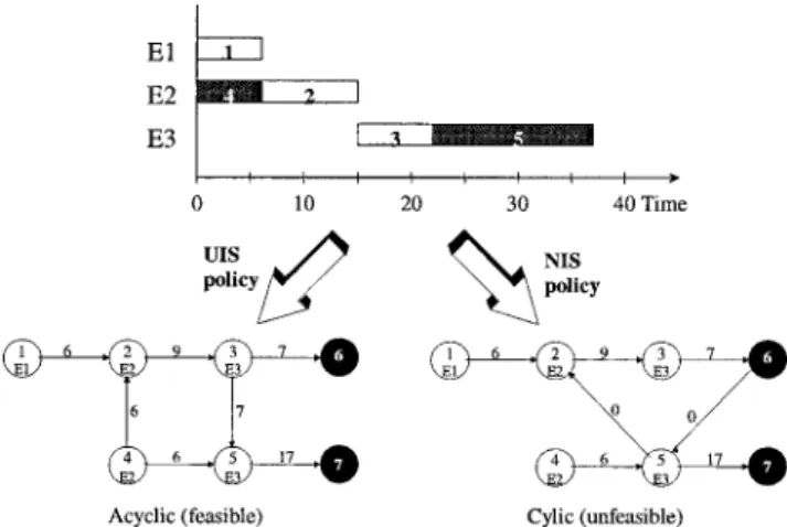
A feasible schedule for the UIS transfer policy may be Figure 2. Optimal UIS and its corresponding NIS policies
infeasible for the NIS case. For instance, Figure 2 shows an optimal Gantt chart for UIS policy, but infeasible for NIS policy. This Gantt chart shows that the transfer of material from equipment unit E1 (task 1) to equipment unit E3 (task 2) simultaneously to the transfer from E3 (task 5) to E1 (task 6) can only be performed if an intermediate storage unit is avail-able to store one of the products while the other is being transferred. The correspondent NIS schedule graph is shown (note that NIS schedule arcs are used). Here two cycles in the graph identify infeasibility. Figure 2 also shows the schedule graph of the same sequence of equipment units, but scheduled with UIS schedule arcs. This sequence is now feasible (not cyclic).
Basic algorithm for optimal scheduling
The recipe graph of a scheduling problem is always a sub-graph of any of its schedule sub-graphs with identical sets of nodes. Extending the recipe graph with arcs in all possible ways by taking into account the set of axioms reported in a previous work (Sanmarti et al., 2002) and constraints on the assign-ments, can therefore result in all schedule graphs. Conse-quently, all schedule graphs and the related assignments can be generated in a finite number of steps. This graph generation can be performed conveniently by a branch and bound (B&B) algorithm, where an equipment unit is assigned to a task and the order of this task is determined in each branching step. In this article the B&B of the basic representation is extended in order to consider common storage units.
Extension of the S-Graph Representation to Consider Intermediate Common Storage
In most batch chemical processes, intermediate storage units are or may be used to increase process flexibility. The CIS policy may include the FIS policy. This is the case when the common storage inlets and outlets are connected to only one equipment unit. Therefore, when solving the CIS policy we are also considering the UIS, NIS, and FIS policies.
Within the CIS policy, an equipment unit is not free after processing a task until the material stored in it has been transferred either to the equipment unit assigned to the next task in the recipe or, if necessary and possible, to an interme-diate storage unit.
Problem definition
Five types of information may define a multipurpose batch-scheduling problem when some interstage storage (IS) is
pos-sible: (a) the recipe of each product, (b) tasks to equipment units assignment, (c) the amount to be produced per product, (d) task to intermediate storage units assignment, and (e) the equipment units to intermediate storage units assignment. The first-three describe the basic scheduling problem. The task to intermediate storage assignment refers to the type of materials that each intermediate storage unit can store. The equipment unit to storage unit assignment describes the physical connec-tivity (hence, flexibility) of the common storage units.
Common Storage Description. The new required informa-tion related to the IS policy is the equipment to intermediate storage assignment and the task to intermediate storage assign-ment. The equipment to intermediate storage assignment infor-mation is included at:
(1) The setISOkof intermediate storage unitsISto which
each equipment unit k can transfer its intermediate products (output materials).
(2) The setISIkof intermediate storage unitsISfrom which
raw materials can be transferred to equipment unit k (input materials).
This information might be enough to properly model the common storage connectivity from a single inlet– outlet to the multiple inlet–multiple outlet intermediate storage unit (Canton et al., 1999).
Specific information should also be given about each inter-mediate storage:
(1) The storage capacity of each intermediate storageIS. (2) The intermediate storage policy, that is, if the intermediate storage is dedicated (used only by one material), shared (can be used by more than one material at the same time), or shared exclusive (can be used a long time by different materials, but only a single material can be in the storage unit at a time).
(3) Tasks to intermediate storage assignment; that is, which type of tasks can or cannot transfer their intermediates to each common storage unitIS.
We can assume that the task to intermediate storage assign-ment is somehow incorporated into the equipassign-ment to interme-diate storage assignment. It is also assumed that if an equip-ment unit is connected to a storage unit, this storage can store its intermediate products. We will also assume that storages are shared exclusively, as this is the most typical situation found in chemical plants.
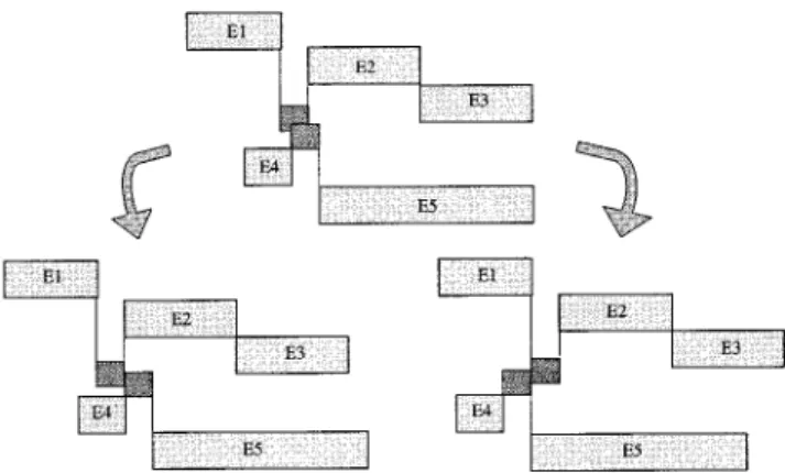
Figure 3. Extended S-graph representation: PT is the task processing time, and TT the transfer times.
Figure 4. S-graph representation of UIS and NIS policy of a batch process.
Storage Representation in the S-Graph. When scheduling batch processes with storage facilities, not only is the sequence of batches decided but so is which route will be used to carry out each batch. Therefore, a kind of mixture of scheduling and synthesis problem is solved. When common storage is consid-ered, the recipe graph should define the order and type of tasks, the set of equipment units of each task, and the feasibility of using an intermediate storage between two adjacent tasks. Since conventional graphs are unable to uniquely represent process structures in synthesis (Friedler et al., 1992), a new type of node will have to be added to the basic representation in order to fully describe the possibility of storage.
In the S-graph representation, tasks are identified by a circle designating the so-called T-type node and products are marked by a dark circle designating the so-called P-type node. In the extended S-graph that considers common storage, the transfer rules between tasks are denoted by a simple arc if no interme-diate storage is used or by a gray circle if storage is used, but also designating a T-type node. In order to represent the chance of choosing between these two paths (one using intermediate storage and the other not) the so-called C-type nodes, desig-nated by black boxes, are introduced. Figure 3 shows the extended recipe-graph of a recipe in which material between nodesiandjcan be transferred either directly or, if necessary, using the set of common storages CISi,j. The set, CISi,j, is
defined as a function of the set of intermediate storage units from which taskjcan transfer its raw materials,ISITj, and the
set of intermediate storage units to which taskican transfer its intermediate products,ISOTi:
CISi,j⫽共ISOTi
艚
ISITj兲. (1)Set of rationales for storage unit necessity and possibility
In order from the outset to reduce the number of partial problems ending in infeasible alternatives derived from using the intermediate storage, a set of rational rules is defined. Such rationales are based on problem-specific knowledge and on the fact that the S-graph is able to exploit this practical insight. This set of concepts will later help to accelerate the optimiza-tion procedure by rejecting nonoptimal and nonfeasible solu-tions before exploring them.
Necessity of Intermediate Storage Rationale. It is easy to determine when an intermediate storage is necessary in a specific schedule graph. Axiom SG1 is established from the basic S-graph representation (Sanmarti et al., 2002). This ax-iom is true for any scheduling policy.
Axiom SG1. A sequence of tasks is feasible if its (partial) schedule graph representation is noncyclic.
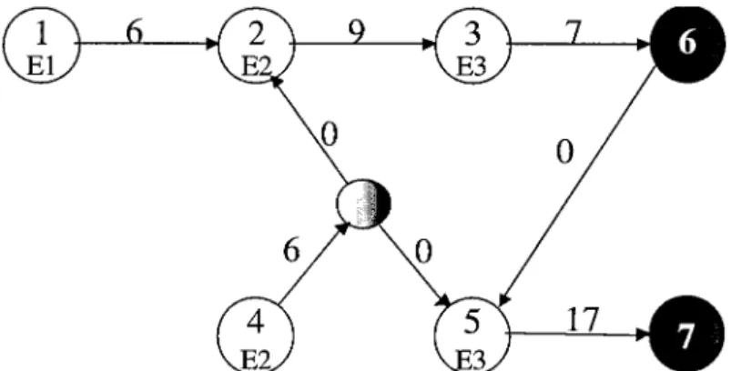
However, as has been previously established, a sequence of tasks may not be feasible in the NIS policy but feasible in the UIS or CIS policy. Figure 4 shows a Gantt chart of a feasible UIS (or maybe CIS) policy, but one that is infeasible within the NIS policy. Their S-graph representation under UIS and NIS Figure 5. Feasible schedule graph of the case in Figure 4 thanks to the introduction of an intermediate storage; C-type
nodes are omitted.
Figure 6. Gantt-chart of the situations found in the non-necessity rules 1 and 2.
Figure 7. Possibility of intermediate storage unit use. PT is the task processing time, TT the transfer time and SU, the setup time of an equipment unit.
Theoverlapping_checkingarc is represented by a dashed arc.
policy is also shown. From this representation it can be seen how a cycle in the NIS case identifies infeasibility.
Figure 5 shows that the cycle detected at the NIS case of Figure 4 is broken by using intermediate storage.
Hence, an infeasible solution at NIS might be transformed into a feasible one by introducing intermediate storage. Using a cycle-detection algorithm, it can be detected when an infea-sible (partial) schedule can be transformed into a feainfea-sible one by introducing intermediate storage. Proposition 1 defines this feasibility.
Proposition 1. Given the set⌰of nodes that form a cycle Ꮿin an S-graphG(N,A1,A2). If for any schedule arc (i,j) (i,
j僐⌻),i, (i⫺1) belongs to⌰, then the S-graphG(N,A1,A2)
is not infeasible because of the precedent node of unavailability of storage.
Demonstration. A cycle in an S-graph defines infeasibility. This infeasibility may be disabled using intermediate storage. In the extended S-graph representation, the intermediate stor-age path implies to change a schedule arc starting at nodei
(representing a task that can be performed by an equipment unit) to one starting at nodeis (representing an intermediate storage that can be performed by a storage unit). As theisnode is connected to nodei⫺1, if nodei⫺1 also belongs to the original set of cycle nodes, the cycle will not be broken by introducing the intermediate storage. If this happens for all schedule arc (i,j)僐⌰, then the infeasibility is not caused by lack of storage. Hence, if arc (i,j) does not exist, cycleᏯwill not be broken if a common storage is available. On the other hand, the S-graph can be transformed into a feasible one introducing, if possible, a new T-type node representing inter-mediate storage.
Nonnecessity of Intermediate Storage Rules. By using a set of rules, it can be known when an intermediate storage being used in a schedule graph is not necessary, either because we can directly transfer intermediates to the next processing unit or because we can store the intermediates in the same processing unit or in the following prior next processing stage. Letibe a batch stage of recipe␣, leti⫹1 be the next stage toiof recipe ␣. Letjbe the next stage scheduled in the same equipment unit asiin the schedule. Letk⫺be the preceding stage scheduled in the same equipment unit asi ⫹1, and letk be the following
stage in the recipe,␣⬘, tok⫺. This set of rules can be summa-rized as follows.
(1) If the earliest scheduled starting time ofi⫹ 1 plus the transfer time and setup time required by taskiis smaller than the latest starting time of j, i can transfer its intermediate products to taski⫹ 1 without having to use an intermediate storage, because if necessary it can store them in the same equipment unit ofi. Figure 6 (rule 1) shows this situation.
(2) If the earliest scheduled finishing time of k⫺ plus its required transfer time and setup time, to transfer its interme-diates tok, is smaller than the latest finishing time ofi,ican also transfer its intermediates to taski⫹ 1 without having to use any external intermediate storage unit. Figure 6 (rule 2) shows this situation.
(3) If there is no task using the same equipment unit asi
scheduled after i (?/ j), or there is no task using the same equipment unit asi⫹1 (?/k⫺), then there is no requirement for intermediate storage.
However, this set of rules does not recognize the necessity of using intermediate storage when a set of equipment units transfer their intermediates one to the other simultaneously. For instance, if in Figure 6,k⫺would be the preceding task in a recipe toj, the transfer represented would be impossible with-out the aid of external intermediate storage. Nevertheless, the necessity of the intermediate storage rule presented before will help to determine when this rule does not recognize this situ-ation. Combining both, it can be known which nodes of a given schedule graph require intermediate storage for transferring their intermediates.
Possibility of Intermediate Storage Rationale. A node can use intermediate storage when transferring its intermediates from taski to taskjifCISi,j⫽ A.
On the other hand, given a schedule graph, it easily can be checked if the use of common intermediate storage overlaps. This checking can be performed by adding arcs from nodej
where the ith use of an intermediate storage discharges its products to the node of the (i⫹1)-th use of this storage. These arcs are calledoverlapping_checkingarcs. Figure 7 shows an instance of this arc: dashed-arc from nodejto nodek⬘. This arc checks whether taski⬘tries to storage its intermediates when intermediates fromiare still in storage unitIS1. The weight of this arc is the transfer time required to transfer the intermediate back to the equipment unit of taskjplus the setup time required to prepare the storage unit for the next intermediate product.
After adding all the possibleoverlapping_checkingarcs be-tween two consecutive uses of each intermediate storage unit, we find the following situations:
(1) No cycle is generated, but makespan is affected after the
overlapping_checkingarcs addition. In this case, the problem is feasible.
(2) A cycle is generated, then the problem is infeasible because of overlapping storage unit use. The only way to avoid the overlapping is to remove theISuses.
(3) No cycle is generated, but makespan is affected after the arc addition. Figure 8 shows this situation. In this case, this means that the schedule graph overlaps theIS use, but this overlap is avoided by dragging some batches with an effect on production makespan. In this situation, there is uncertainty in the schedule-graph information as to which IS is, in fact, being used first. Hence, bothISuse orders should be considered. Figure 8. Case where the addition of
overlapping-_checkingarcs does not generate a cycle but
Optimization strategy
Given all this information, the optimization procedure will look for the optimal sequence of tasks (with lower production makespan) to meet the specified requirements that allow, if possible, the storage of some intermediate products.
The S-graph procedure will be applied in order to find the
optimal schedule. Within this framework, three strategies could be possible:
● Exhaustive B&B, solving the problem considering all the possibilities and paths between each two nodes, that is, at each sequence step of each equipment unit, when a C-type node is found, consider the transfer using intermediate storage and the Figure 9. Examples of schedule graphs using the set of rationales for storage use and possibility.
transfer without using storage, and so generate two subprob-lems.
● First solve the problem without using the possibility of using intermediate storage, and introducing the storage path when necessary to make feasible the schedule and whenever possible to increase productivity.
● First solve the problem by always choosing the interme-diate storage path at each P-type node and introduce NIS-schedulearcs when the intermediate storage unit is not neces-sary and/or not possible.
The exhaustive B&B strategy implies schedule equipment units generating two subproblems from any partial problem: One with a NIS transfer and another with UIS transfer. In this way, when a complete schedule is obtained (schedule graph), intermediate storage use is checked, adding the overlapping-_checking_arcsfrom eachith use to the (i⫹1)-th use of each storage unit. This strategy is not computationally efficient, as it generates two subproblems from each P-type node that is found. Hence, it can be used only to solve small problems. However, as this strategy is not based in any rationale, opti-mality is guaranteed.
As for the second strategy, it is difficult to determine when the use of intermediate storage will increase final productivity (reduce makespan) of a given S-graph. Therefore, it is dis-carded.
As a computationally efficient optimization strategy, we choose to initially solve the problem, always choosing, if it exists, the intermediate storage path by expanding the tree with
UIS-schedule arcs and introducing NIS-schedule arcs when storage is not necessary and/or not possible. Specifically, the steps to follow are:
(1) Start branching partial problems by addingUIS-schedule
arcs in place of each P-type node. Otherwise, add a
NIS-schedulearc. With this, on the one hand, the use of storage is probably assumed when not necessary and, on the other, their use may overlap. Nevertheless, the lower bound of any of these partial problems will always be lower than or equal to any feasible one, and therefore there is no lose of optimality when bounding the searching tree with these partial problems.
(2) Once a complete schedule is obtained, check to see which nodes of those scheduled to use the storage paths need to use common storage. Those nodes transferring their mate-rials using the storage paths not requiring common storage are changed toNIS-schedulearcs. In order to perform this, see if it is necessary, or not, to use the intermediate storage rules described earlier.
(3) Finally, check to see if tasks try to store their interme-diates in the same storage at the same time, that is, if there is infeasibility in the use of the storage unit. For this, the schedule graph is extended to incorporate the storage nodes, as shown in Figure 4, and the possibility of intermediate storage rationale described earlier is used. When overlapping is detected, all possible combinations of intermediate storage use removal are considered, until a feasible IS use is found or the solution is discarded (because it is infeasible).
Algorithm for computationally optimal CIS policy scheduling
The optimal schedule is determined by applying the B&B framework of the S-graph representation. Each node in the B&B algorithm tree corresponds to a partial schedule. At the root of the tree, the only earlier constraints of the product recipes are applied, that is, the S-graph contains no arcs rep-resenting task sequences in the units. For this graph, the back-wardlongest path algorithmcan be applied to obtain a lower bound of the makespan. Then, the tasks assigned to the differ-ent units are sequenced one by one. Each time a task is sequenced, a branch is generated in the tree, and the longest path algorithm is applied again if no cycle is detected on the graph. When the tree reaches the bottom, a complete schedule has been obtained and a lower bound of the makespan can be calculated. The Appendix shows the main procedure and the different parts of the B&B algorithm.
Thelongest path algorithmassumes that unlimited waiting times are allowed. If this is not the case, the lower bound of the makespan has to be calculated using a linear programming (LP) model. Later, in Example 1, a LP formulation to be solved in this situation is shown.
Each time the lower bound of a partial schedule is greater than the current upper bound, or that the partial schedule is not acyclic, the branch of study is pruned.
This B&B algorithm is divided into the following procedures (according to optimization strategy 3).
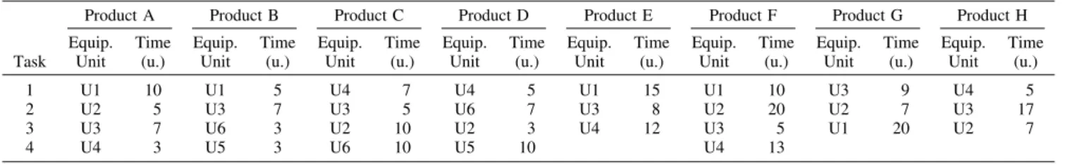
Table 1. Recipes Used for Algorithm Evaluation
Task
Product A Product B Product C Product D Product E Product F Product G Product H Equip. Unit Time (u.) Equip. Unit Time (u.) Equip. Unit Time (u.) Equip. Unit Time (u.) Equip. Unit Time (u.) Equip. Unit Time (u.) Equip. Unit Time (u.) Equip. Unit Time (u.) 1 U1 10 U1 5 U4 7 U4 5 U1 15 U1 10 U3 9 U4 5 2 U2 5 U3 7 U3 5 U6 7 U3 8 U2 20 U2 7 U3 17 3 U3 7 U6 3 U2 10 U2 3 U4 12 U3 5 U1 20 U2 7 4 U4 3 U5 3 U6 10 U5 10 U4 13
The Branching Procedure. The recipe graph serves as a root of the searching tree. At any partial problem, one equip-ment unit is selected and all child partial problems are gener-ated through the possible assignments of this equipment unit to unscheduled tasks. If available, the storage path is always chosen. This procedure uses a backtracking search strategy. When a cycle is detected, the study branch is pruned. The Appendix shows this procedure. For simplicity, it is assumed that there is exactly one equipment unit to perform each task. There is a high degree of freedom in realizing the branching algorithm to select the appropriate or most effective search strategy.
The Bounding Procedure. The bounding procedure tests the feasibility of a partial problem by first using a cycle search
algorithm. If the partial problem is acyclic, it returns a lower bound for the makespan of all solutions that can be derived from this partial problem.
TheIS_necessityProcedure. At the end of the tree, where each feasible solution is reached (schedule graph), the proce-dureIS_necessityis called. For simplicity, it is assumed that at most only one intermediate storage is connected to each input/ output of each equipment unit. In addition, there is not much sense in connecting more than one storage unit to the same equipment unit. This assumption makes the set of nodes re-quiring external storage after processing,ISNi, single for alli
(i ⫽ 1, 2, . . . , n).
This procedure uses the nonnecessity concept described earlier to identify which nodes are in fact using the inter-mediate storage. If the nonnecessity rules consider a node requiring storage to be nonrequiring, the resultant graph will be cyclic. This is the case of a set of equipment units simultaneously transferring their intermediates one to the other (the case of Figure 6 wherek⫺is the task in the recipe that precedesj). If happens, theIS necessityrationale (called theIS_cycle_breakingprocedure) is used to identify which nodes in fact require storage. Once all nodes requiring intermediate storage are known, the IS_overlapping_check
procedure is called. The Appendix shows the IS_necessity
procedure.
The IS_cycle_breaking Procedure. This procedure is called when a cycle is detected within the IS_necessity
procedure. This procedure looks for the set of nodes that by using intermediate storage instead of direct transfer will break the cycle. This procedure is based on the intermediate storage necessity rationale introduced earlier. See the Ap-pendix for the IS_cycle_breaking procedure when there is only one storage shared among equipment units. In this situation, using the storage⫹unit is the same wherever we break the cycle by means of intermediate storage, and hence, it is not necessary to search for all the possible cycle-breaking points.
The IS_overlapping_check Procedure. This procedure checks to see if the use of intermediate storage is infeasi-ble, that is, if more than one equipment unit is trying to store its intermediates in the same storage unit at the same time. This procedure first adds storage arcs from the ith use of every intermediate storage unit to its (i⫹1)-th use. If the resulting graph is acyclic, the use of storages is feasible. Otherwise, the cycle_remove procedure is called (see the Appendix).
The Cycle–remove Procedure. Here, one intermediate storage use is removed after considering all possible uses. For each storage use, the procedure removes it and stores the new
schedule-graphfor a new IS overlapping check (see the Ap-pendix).
Table 2. Randomly Generated Input Data for Algorithm Evaluation
Scenario
Number of Batches of Product
A B C D E F G H 1 1 1 1 1 0 0 0 0 2 0 0 0 0 1 1 1 1 3 0 1 1 0 2 0 0 0 4 0 0 0 1 0 1 1 1 5 1 0 1 0 1 0 1 0 6 1 1 1 0 1 0 2 0 7 1 0 1 0 1 0 0 1 8 1 0 1 0 1 0 1 1 9 2 1 0 0 0 1 1 0 10 2 1 0 0 0 0 0 2 11 2 2 0 0 0 0 0 1 12 1 2 0 1 0 0 0 0 13 1 0 2 1 0 0 0 0 14 0 0 0 0 3 0 0 1 15 0 0 2 0 1 1 0 0 16 1 0 0 0 0 1 0 2 17 0 2 0 0 0 0 3 0 18 2 0 0 0 2 0 1 0 19 1 1 0 0 0 0 0 2 20 1 1 0 0 1 1 0 0
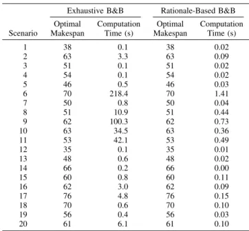
Table 3. Exhaustive vs. Rationale-Based Algorithm Evaluation
Scenario
Exhaustive B&B Rationale-Based B&B Optimal Makespan Computation Time (s) Optimal Makespan Computation Time (s) 1 38 0.1 38 0.02 2 63 3.3 63 0.09 3 51 0.1 51 0.02 4 54 0.1 54 0.02 5 46 0.5 46 0.03 6 70 218.4 70 1.41 7 50 0.8 50 0.04 8 51 10.9 51 0.44 9 62 100.3 62 0.73 10 63 34.5 63 0.36 11 53 42.1 53 0.49 12 35 0.1 35 0.01 13 48 0.6 48 0.02 14 66 0.2 66 0.00 15 60 0.8 60 0.11 16 62 3.0 62 0.09 17 76 4.8 76 0.15 18 70 0.6 70 0.10 19 56 0.4 56 0.03 20 61 6.1 61 0.10
Table 4. Processing and Transfer Times for Example 1
Product
Processing Time (u.) Transfer Time (u.) U1 U2 U3 U4 U5 U6 U0 U1 U2 U3 U4 U5 U6
P1 10 15 20 12 8 11 2 2 2 2 3 2 1
P2 15 8 12 10 9 13 3 3 3 3 1 1 2
P3 10 22 9 5 6 9 2 4 2 2 1 2 2
Illustrative example
This illustrative example consists of scheduling the produc-tion of two batches of two different products using two equip-ment units. The recipe graph is shown in Figure 9 (partial problem No. 1). It is assumed that one common storage unit is available to all equipment units. For clarity C-type nodes are not shown. The search tree is given in Figure 10. The nodes of the tree represent the partial problems. The branches are iden-tified by the task sequence they introduce. The lower bound associated with each of the feasible partial problems is shown in boldface. The node of an infeasible partial problem is crossed. The part of the searching tree not to be explored by the optimization strategy is shown by dashed lines. The S-graphs that correspond to these partial problems are shown in Figure 9. The root of the search tree (partial problem No. 1) corre-sponds to the recipe graph; the longest path, a lower bound of its makespan, is 9. From this partial problem, two branches,
partial problem No. 2andNo. 3,are generated for the sequence of equipment unit E1: 1– 4 and 4 –1, with lower bounds of 9 and 16, respectively. The branch with the best lower bound is
partial problem No. 2,and it is selected to continue expanding the tree. From this partial problem, two branches (partial problem No. 4andNo. 5) are generated: sequences 2–3 and 3–2 for equipment unit E2. Both partial problems are complete schedules, that is, they may lead to a new upper bound for the minimum makespan.Partial problem No. 4represents a
com-plete schedule with a makespan of 16, then it checks to see which of the nodes scheduled using the UIS arcs need to use common storage (the necessity and nonnecessity of intermedi-ate storage rationales are used for this). Those nodes not requiring common storage are changed toNIS-schedulearcs. Since no node requires storage, the graph does not need to be extended to consider them (partial problem No. 4⬘). Now, the lower bound of this partial problem is an upper bound for the optimal makespan. Therefore, partial problem No. 3 is dis-carded, as its bound is equal to the actual upper bound and all of its descendants will have a bound equal or higher than it.
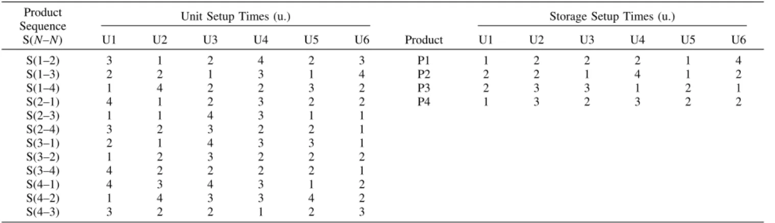
Partial problem No. 5has a lower bound of 9. After checking to see which nodes need to use common storage (using the necessity and nonnecessity of intermediate storage rationales), the nodes not requiring common storage are changed to NIS-schedulearcs and, at the node requiring storage, node 3, the graph is extended to consider it (partial problem No. 5⬘). Since there is only one storage unit in use, it is not necessary to check for storage unit overlap. Now, the lower bound of this partial problem (9) is an upper bound for the optimal makespan. Therefore,partial problem No. 4⬘is discarded.Partial problem No. 3would be the next branch to be expanded, from which sequences 2–3 and 3–2 for equipment unit E2 would be gen-erated. However, they are not to be explored, since the lower bound of their ancestor (partial problem No. 3) is not better (lower) than the current upper bound. Now, there are no more Table 5. Setup Times for Equipment and Storage Units of Example 1
Product Sequence
S(N–N)
Unit Setup Times (u.)
Product
Storage Setup Times (u.)
U1 U2 U3 U4 U5 U6 U1 U2 U3 U4 U5 U6 S(1–2) 3 1 2 4 2 3 P1 1 2 2 2 1 4 S(1–3) 2 2 1 3 1 4 P2 2 2 1 4 1 2 S(1–4) 1 4 2 2 3 2 P3 2 3 3 1 2 1 S(2–1) 4 1 2 3 2 2 P4 1 3 2 3 2 2 S(2–3) 1 1 4 3 1 1 S(2–4) 3 2 3 2 2 1 S(3–1) 2 1 4 3 3 1 S(3–2) 1 2 3 2 2 2 S(3–4) 4 2 2 2 2 1 S(4–1) 4 3 4 3 1 2 S(4–2) 1 4 3 3 4 2 S(4–3) 3 2 2 1 2 3
Figure 11. Optimal schedule graph of multiproduct Example 1; the weight of the arcs show the processing times, transfer times, and setup times.
nodes to expand, therefore, the optimal solution is given by
partial problem No. 5⬘.
Algorithm Performance
In order to show the accuracy of combining the set of proposed rationales with the S-graph B&B, a set of randomly generated input data is solved using the exhaustive optimiza-tion strategy and the raoptimiza-tionales-based strategy. In this evalua-tion, six equipment units, U1, U2, U3, U4, U5, and U6, are available to generate eight products, products A to H. The recipes of the products are given in Table 1, which shows that one common storage is available at the inlet and outlet of each equipment unit. Twenty randomly generated scenarios for eval-uation are given in Table 2.
The exhaustive B&B guarantees optimality. Table 3 shows that the exhaustive and the rationales-based approaches always reach the same optimal makespan. Therefore, as was expected, it can be concluded that the set of rationales does not exclude any optimal solution of the B&B exploration. Table 3 also shows that the rationales-based B&B is considerably more computational efficient than the exhaustive one.
Program Realizations and Applications
To evaluate the proposed graph-theoretical algorithm perfor-mance, three examples are examined. The first one considers a multiproduct plant producing four different products in six processing units. Setup (switchover) times for units and stor-age, transfer times, and zero waiting (ZW) blocks are taken into
account in this example. The next example contemplates a multipurpose batch plant. The next case has already been studied in the literature and here we refute the literature solu-tions. The last example contemplates a large multipurpose case study, where setup times are taken into account.
Example 1
This example was proposed by Jung et al. (1996). The plant is a serial-flow shop system that has four batches carried out in six equipment units, U1, U2, U3, U4, U5, and U6, with one common storage unit IS1 shared among equipment units. Table 4 shows the data used for this example. Setup times as a function of the equipment unit and recipe sequence have been taken into account, as shown in Table 5.
A ZW block is assumed between units 3 and 5. In order to consider the ZW block, the LP problem shown in Eq. 2 is solved. This LP is used to bound partial problems instead of the longest path algorithm that assumes unlimited waiting times
min MS
TIiⱖ0 ᭙i
TFi⫽TIi⫹TOPi⫹TWi ᭙i TFi⫽TIi⬘ ᭙共i,i⬘兲僐A1
TFi⫺1ⱕTIi⬘ ᭙共i,i⬘兲僐A2
TWiⱕTWi
max ᭙i
MSⱕTFi ᭙i, (2)
whereTIiandTFiare the initial time and ending time of each
process stagei;TWi max
is the maximum waiting time allowed, equal to 0 ifi belongs to the ZW block;TOPithe processing
time of taski:MSis the production makespan:A1 represents
the set of recipe arcs of a partial problem; andA2stands for the
set of schedule arcs.
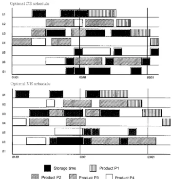
The optimal NIS production makespan is of 144 u. We suggest that the common intermediate storage production makespan is reduced to 136 u. This is the same value as reported by Jung et al. (1996). However, our framework allows storage of intermediates in the same equipment unit whenever possible, a fact not contemplated in the original solution. For Figure 12. Optimal Gantt charts of multipurpose
Exam-ple 2 when scheduling one batch of product A, three of B, two of C, and one of D, when a common storage unit is available, and when no storage unit is available.
Figure 13. Infeasible optimal Gantt chart proposed by Kim et al. (2000) and optimal feasible Gantt chart according to the S-graph algorithm.
this reason, our actual solution differs from the one reported. In our optimal solution, storage is required after processing prod-ucts P2 and P3 in equipment unit U2. This storage is performed at the common storage, since U2 is required for further pro-cessing. Storage is also required after processing product P3 in equipment unit U5, but here it is possible to perform this storage in the same equipment unit, U5, a situation not con-templated by Jung et al. Figure 11 shows the optimal schedule graph of this example. In this figure we can see the differences between the weight of the arcs among processing time, transfer times, and setup times.
Example 2
In this example six equipment units, U1, U2, U3, U4, U5, and U6, are available to generate four products, products A, B, C, and D of Table 1. One common storage unit is available at the inlet and outlet of each equipment unit. In this example, transfer and setup times have been considered negligible, and no waiting time limitations are assumed.
Figure 12 shows the optimal Gantt chart for producing one batch of product A, three of B, two of C, and one of product P4 when common storage is available (optimal CIS schedule) and in the case where no intermediate storage is allowed (optimal NIS schedule). The optimal solution for CIS is achieved in 32 CPU seconds in a 1-GHz machine. By introducing the common storage the production makespan is reduced from 56 u to 52 u. The optimal CIS Gantt chart shows that the intermediate stor-age unit is first used from the outlet of equipment unit U6 to the inlet of U2, then from the outlet of U1 to the inlet of U3, then
from the outlet of U1 to the inlet of U3, and finally from the outlet of U3 to the inlet of U6. Therefore, our algorithm properly exploits the flexibility of the common storage unit to increase productivity by 8%. The optimal UIS schedule has a makespan of 51 u, and would be feasible if two common storage units were available.
Example 3
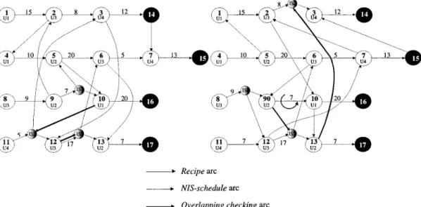
In this example, the nonsequential multipurpose process proposed by Kim et al. (2000) is solved using the S-graph approach. The process produces four products using four units. These products correspond to products E, F, G, and H of Table 1. The optimal solution reported by Kim et al. (2000) requires a production makespan of 60 u obtained in 1.24 CPU s using an IBM RS/6000 (model 350). Our optimal solution shows a production makespan of 63 u, obtained in 0.08 CPU s of a 1-GHz machine. However, the solution reported in the work of Kim et al. is not feasible (see Figure 13) because the transfer of product B from unit 2 to unit 3 first requires the transfer of product D to storage. But, in order to transfer product D, product C needs to be transferred from storage to unit 2, which requires the transfer of product B. This is impossible if no other external storage unit is available. In the S-graph representation, this infeasible situation is identified by a cyclic graph. Figure 14 shows our optimal feasible schedule graph and the schedule graph of the solution proposed by Kim et al. (2000). It can be observed that this second solution is feasible before adding the
overlapping– checking arcs, but after adding them, a cycle,
Table 6. Recipes Used for Example 4
Task
Product 1 Product 2 Product 3 Product 4 Product 5 Product 6 Product 7 Product 8 Equip. Unit Time (u.) Equip. Unit Time (u.) Equip. Unit Time (u.) Equip. Unit Time (u.) Equip. Unit Time (u.) Equip. Unit Time (u.) Equip. Unit Time (u.) Equip. Unit Time (u.) 1 U1 100 U2 150 U13 280 U14 260 U5 350 U1 120 U2 300 U3 260 2 U2 450 U10 90 U8 300 U9 190 U10 120 U6 130 U7 50 U8 200
3 U14 400 U12 240 U3 250 U4 300 U15 420 U11 300 U12 250 U12 250
Figure 14. Infeasible schedule graph representation of the solution proposed by Kim et al. (2000) and optimal feasible schedule graph according to the S-graph algorithm.
generated in nodes 11, IS2, and 7 identifies infeasibility in the storage unit use.
Example 4
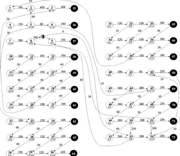
Fifteen equipment units, U1 through U15, are available to generate eight products, 1 to 8. The recipes of the products are given in Table 6. The changeover time is 10 min for equipment units U1, U12, and U13, 30 min for equipment units U8, U9, U10, U11, U14, and U15, and 60 min for equipment units U2, U3, U4, U5, U6, and U7. One storage unit to share among all equipment units is available. Changeover time for the storage unit is zero. The number of batches to be produced is given in Table 7 for each product. The problem was solved in 132-s CPU time on a AMD-Athlon 1 GHz machine. The resultant makespan is of 1910 min. Figure 15 shows the corresponding schedule graph.
Concluding Remarks
This study demonstrates that the proposed graph-theoretical approach S-graph for scheduling multiproduct and multipur-pose batch plants with shared storage is feasible and efficient. The basic algorithm of the S-graph has been extended by first introducing a new type of node in the graph that represents the possibility of using intermediate storage (C-type node). In order to efficiently solve the problem, the exploration tree is reduced from the beginning by using a set of rationales. In the proposed algorithm, the problem is initially solved by always choosing the storage path if available. Once a schedule graph is obtained, storage use necessity and graph feasibility are ana-lyzed. This procedure guarantees optimality, as the lower bound of any of the S-graphs obtained by always choosing the storage path always will be lower or equal to any respective feasible schedule graph. A set of rationales determines whether a given schedule graph storage unit use is infeasible. If it is, all of the possible IS unit allocations are considered for removal until use of the IS unit in the schedule graph becomes feasible; otherwise, the subproblem is discarded. This algorithm has been tested in multiproduct and multipurpose batch-plant case studies, showing the performance and accuracy of the method. Table 7. Number of Batches of the Products
Product 1 2 3 4 5 6 7 8
Number of batches 1 1 1 4 3 3 1 4
Acknowledgment
One of the authors (J.R.) acknowledges a grant from theGeneralitat de Catalunya.This research has been supported in part by the Hungarian National Science Foundation OTKA T-029-309 and by the European community (CHEM project n G1RD-CT-2001-00466).
Literature Cited
Adams, J., E. Balas, and D. Zawack, “The Shifting Bottleneck Procedure for Job Shop Scheduling,”Manage. Sci.,34, 391 (1988).
Canton, J., M. Graells, and L. Puigjaner, “Modeling Intermediate Storage for the Scheduling of Multipurpose Batch Chemical Processes Using Event Operation Networks,” AIChE Meeting, Dallas, TX (1999). Friedler, F., K. Tarjn, Y. Huang, and L. Fan, “Graph-Theoretic Approach to
Process Systhesis: Axions and Theorems,”Chem. Eng. Sci.,47, 1973 (1992). Holczinger, T., J. Romero, L. Puigjaner, and F. Friedler, “Scheduling of Multipurpose Batch Processes with Multiple Batches of the Products,”
Hungarian J. Ind. Chem.,30, 305 (2002).
Ierapetritou, M., and C. Floudas, “Short-Term Scheduling: New Mathe-matical Models vs. Algorithmic Improvements,”Comput. Chem. Eng., 22, S419 (1998).
Jung, J., H. Lee, and I. Lee, “Completion Times Algorithm of Multi-Product Batch Processes for Common Intermediate Storage Policy (cis) with Nonzero Transfer and Set-Up Times,”Comput. Chem. Eng.,20, 845 (1996).
Kim, M., J. Jung, and I. Lee, “Optimal Scheduling of Multi-Product Batch Processes for Various Intermediate Storage Policies,”Ind. Eng. Chem. Res.,35, 4058 (1996).
Kim, S., H. Lee, I. Lee, E. Lee, and B. Lee, “Scheduling of Non-Sequential Multipurpose Batch Processes Under Finite Intermediate Storage Pol-icy,”Comput. Chem. Eng.,24, 1603 (2000).
Kondili, E., C. Pantelides, and R. Sargent, “A General Algorithm for Short-Term Scheduling of Batch Operations—i. MILP Formulation,”
Comput. Chem. Eng.,17(2), 211 (1993).
Ku, H., and I. Karimi, “Scheduling in Serial Multi-Product Batch Processes with Finite Interstage Storage: A Mixed Integer Linear Program Formu-lation,”Ind. Eng. Chem. Res.,27, 1840 (1988).
Ku, H., and I. Karimi, “Completion Time Algorithms for Serial Multiproduct Batch Processes with Shared Storage,”Comput. Chem. Eng.,14, 49 (1990). Mokashi, S., and A. Kokossis, “Maximum Oder Tree Algorithm for Optimal Scheduling of Product Distribution Lines,”AIChE J.,48(2), 287 (2002). Pinto, J., and I. Grossmann, “A Continuous Time Mixed Integer Linear
Programming Model for Short Term Scheduling of Multistage Batch Plants,”Ind. Eng. Chem. Res.,34, 3037 (1995).
Pinto, J., and I. Grossmann, “Assignment and Sequencing Models of the Scheduling of Process Systems,”Ann. Oper. Res.,81, 433 (1998). Reklaitis, G., “Perspectives on Scheduling and Planning of Process
Oper-ations,” Proc. Int. Symp. on Process System Engineering, Montreal, Canada (1991).
Sanmarti, E., T. Holczinger, L. Puigjaner, and F. Friedler, “Combinatorial Framework for Effective Scheduling of Multipurpose Batch Plants,”
AIChE J.,48(11), 2557 (2002).
Schilling, G., and C. Pantelides, “A Simple Continuous-Time Process Scheduling Formulation and a Novel Solution Algorithm,” Comput. Chem. Eng.,20, S1221 (1996).
Shah, N., “Single and Multisite Planning and Scheduling: Current Status and Future Challenges,”Foundations of Computer Aided Process Op-erations, AIChE Symp. Ser.,94(320), 91 (1998).
Voudouris, V., and I. Grossmann, “MILP Model for Scheduling and Design of a Special Class of Multipurpose Batch Plants,” Comput. Chem. Eng.,20(11), 1335 (1996).
Wiede, W., “An Interactive Scheduling System for the Operation of Multi-Product Plants,” PhD Diss., Purdue Univ., West Lafayette, IN (1984). Appendix
This Appendix gives a detailed algorithm description of the rationale-based CIS production scheduling method presented. The Main procedure of the CIS scheduling algorithm:
proceduremain
notation:
n: number of equipment units
Ni(i⫽1, 2, . . . ,n): set of tasks that can be performed
by equipment uniti
last_node:set of pairs (i,j) whereiis an equipment unit andjis a node.
PP ⫽ (G(N,A1,A2), bound, last_node, SOU N)
input:recipe-graphG(N,A1,A) andNi(i⫽1, 2, . . . ,n)
begin
SET ⫽A; bound ⫽ 0;SOU N ⫽ N1 艛 N2 艛. . .艛
Nn;
last_node ⫽ A; current_best ⫽ ⬁;
Put (G(N,A1,A), bound,last_node,SOU N) intoSET;
while SET ⫽A do
Select and remove elementGfromSET, being denoted byPP;branching (PP);
end end
Branching(PP) procedure: procedurebranching(PP)
comment:generatesall child partial of partial problemPP
notation:graph(PP) ⫽G(N, A1, A2) bound(PP) ⫽ bound
last_node(PP) ⫽ last_node SOU N(PP) ⫽ SOU N
begin
letEQbe an equipment unit that can be assigned to an unscheduled node;
let SO ⫽ NEQ 艚SOU N(PP);
for all k 僐SO do
ifthere is no pair (i,j)僐 last_node 兩 i ⫽EQ then
Put(graph(PP), bound(PP), last_node(PP) 艛 {EQ,k},
SOU N(PP) \ k}) into SET; else letGo(N,A1,A2) ⫽ graph(PP); for all(j, l) 僐A1 do updatec(j,l); Go(N, A1, A2) ⫽ Go(N,A1,A2 艛 {(l,k)}); end bounding(Go(N, A1 艛 A2), bound);
ifbound ⬍ current_best then ifSOU N(PP) \ k ⫽ A then
IS_necessity(Go(N, A1, A2));
else
Put(Go(N,A1,A2),bound,last_node(PP)艛{EQ,
k} \ {EQ,j},SOU N(PP) \k})into SET; end end end end end IS_necessity(G)procedure: procedureIS_necessity(G(N,A1,A2))
comment:checks the necessity of intermediate storage notation:next(i): Node using the same equipment unit just
after nodei.
prev(j): Node using the same equipment unit just before nodej.
dj: Longest distance of nodej from all product nodes
when bounding G.
ISNis: Set of nodes requiring to store their intermediates
in storage unitis. begin
for all i 僐ISN do ifnext(i) ⫽ Athen ISN ⫽ ISN\i; else j ⫽ next(i); ifdi⫹1 ⱖ dj then ISN ⫽ ISN \ i; end end if prev(i ⫹ 1) ⫽ Athen ISN ⫽ ISN\i; else k ⫽ prev(i ⫹ 1); if(dk ⫺ c(k, k ⫹ 1) ⱖ (di ⫺ c(i, i ⫹ 1)) then ISN ⫽ ISN\i; end end end
update G(N, A1, A2) with ISN;
ifbounding(G(N, A1,A2)) ⫽ ⬁ do
IS_cycle_break(G(N, A1, A2));
end
if兩ISNis兩 ⱕ 1 @is then
bounding(G(N, A1, A2), bound);
ifbound ⬍ current_best then
update SET, current_best, solution; end else ISSET ⫽ A; IS_overlapping_check(G); end end IS_cycle_breaking(G)procedure:
procedureIS_cycle_breaking(G(N,A1,A2))
comment:Procedure for breaking graph-cycles by introduc-ing IS
notation:⌰; Set of nodes forming a cycle
ISN;Set of nodes requiring to store their intermediates begin
for all (i, j) 僐A2 do
if i僐 ⌰ andCISi,j⫽ A and(i ⫺1) 苸 ⌰ then change(i, j) for the storage path;
ISN ⫽ ISN 艛 (i ⫺ 1);
ifcycle_search(G(N,A1,A2)) ⫽ cycle then
return; end end end end IS_overlapping_check(G)procedure:
procedureIS_overlapping_check(G0(N, A1,A2))
comment:Checks timing feasibility of the storage units use and if overlapping tries to solve the conflict
begin
bounding(G0)N, A1, A2), bound0);
put G0(N, A1, A2), bound0 into ISSET;
while ISSET ⫽ A do
Remove element {G1(N,A1,A2),bound1} from ISSET;
for all use i 僐 ISdo
ifthere isi ⫹1thuse of storagethen
is_overlap ⫽ false;
extendG1(N,A1,A2) by an arc from theith use
of storage to its i⫹1th use;
ifcycle_search(G1(N,A1,A2)) ⫽ cycle then
is_overlap ⫽ true;
cycle_remove(G1(N, A1, A2));
else
bounding(G1(N,A1,A2), bound);
ifbound ⬎ bound1 then
bound1 ⫽ bound;
is_overlap ⫽ true; end
ifis_overlap ⫽true then
G2(N,A1 A2) ⫽ G0(N,A1,A2);
extendG2(N,A1,A2) by an schedule-arc from
the i⫹1th use of storage to its ith use; ifcycle_search(G1(N,A1,A2))⫽cyclethen
cycle_remove(G2(N, A1, A2));
else
bounding(G2(N, A1, A2), bound2);
ifbound ⬍ current_best then
Put {G0(N,A1,A2),bound1} into ISSET;
end end end end
ifbound1 ⬍ current_best then
update SET, ISSET,current_best and solution end
end
Cycle_removes(G)procedure:
procedureCycle_remove(G(N,A1,A2))
comment:Removes IS use to resolve storage unit use over-lapping begin for all i 僐⌰ do Gis(N, A1, A2) ⫽ G(N,A1,A2) ifi 僐 ISN then ISN \ i;
update Gis(N, A1, A2) with ISN;
ifcycle_search(Gis(N,A1,A2)) ⫽ cycle then
bounding(Gis(N,A1,A2), bound);
If bound ⬍ current_best then
Put {Gis(N, A1, A2), bound} into ISSET;
end end end end end