https://doi.org/10.5194/gmd-13-2959-2020 © Author(s) 2020. This work is distributed under the Creative Commons Attribution 4.0 License.
Surrogate-assisted Bayesian inversion for landscape
and basin evolution models
Rohitash Chandra1,2, Danial Azam2, Arpit Kapoor3, and R. Dietmar Müller2
1School of Mathematics and Statistics, University of New South Wales, Sydney, NSW 2052, Australia 2EarthByte Group, School of Geosciences, University of Sydney, Sydney, NSW 2006, Australia
3Department of Computer Science and Engineering, SRM Institute of Science and Technology, Tamil Nadu, India Correspondence:Rohitash Chandra ([email protected])
Received: 9 December 2018 – Discussion started: 20 February 2019 Revised: 30 March 2020 – Accepted: 6 June 2020 – Published: 8 July 2020
Abstract. The complex and computationally expensive na-ture of landscape evolution models poses significant chal-lenges to the inference and optimization of unknown model parameters. Bayesian inference provides a methodology for estimation and uncertainty quantification of unknown model parameters. In our previous work, we developed parallel tem-pering Bayeslands as a framework for parameter estima-tion and uncertainty quantificaestima-tion for the Badlands land-scape evolution model. Parallel tempering Bayeslands fea-tures high-performance computing that can feature dozens of processing cores running in parallel to enhance computa-tional efficiency. Nevertheless, the procedure remains com-putationally challenging since thousands of samples need to be drawn and evaluated. In large-scale landscape evolution problems, a single model evaluation can take from several minutes to hours and in some instances, even days or weeks. Surrogate-assisted optimization has been used for several computationally expensive engineering problems which mo-tivate its use in optimization and inference of complex geo-scientific models. The use of surrogate models can speed up parallel tempering Bayeslands by developing computation-ally inexpensive models to mimic expensive ones. In this pa-per, we apply surrogate-assisted parallel tempering where the surrogate mimics a landscape evolution model by estimating the likelihood function from the model. We employ a neural-network-based surrogate model that learns from the history of samples generated. The entire framework is developed in a parallel computing infrastructure to take advantage of paral-lelism. The results show that the proposed methodology is ef-fective in lowering the computational cost significantly while retaining the quality of model predictions.
1 Introduction
The Bayesian methodology provides a probabilistic approach for the estimation of unknown parameters in complex mod-els (Sambridge, 1999; Neal, 1996; Chandra et al., 2019b). We can view a deterministic geophysical forward model as a probabilistic model via Bayesian inference, which is also known as Bayesian inversion, which has been used for land-scape evolution (Chandra et al., 2019a, c), geological reef evolution models (Pall et al., 2020), and other geoscien-tific models (Sambridge, 1999, 2013; Scalzo et al., 2019; Olierook et al., 2020). Markov chain Monte Carlo (MCMC) sampling is typically used to implement Bayesian inference that involves the estimation and uncertainty quantification of unknown parameters (Hastings, 1970; Metropolis et al., 1953; Neal, 2012, 1996). Parallel tempering MCMC (Mari-nari and Parisi, 1992; Geyer and Thompson, 1995) features multiple replicas to provide a balance between exploration and exploitation, which makes them suitable for irregular and multimodal distributions (Patriksson and van der Spoel, 2008; Hukushima and Nemoto, 1996). In contrast to canoni-cal sampling methods, we can implement parallel tempering more easily in a parallel computing architecture (Lamport, 1986).
Our previous work presented parallel tempering Bayeslands for parameter estimation and uncertainty quantification for landscape evolution models (LEMs) (Chandra et al., 2019c). Parallel tempering Bayeslands features parallel computing to enhance computational efficiency of inference for the Badlands LEM. Although we used parallel computing, the procedure was computationally challenging since thousands of samples were drawn and
evaluated (Chandra et al., 2019c). In large-scale LEMs, running a single model can take several hours, to days or weeks, and usually thousands of model runs are required for inference of unknown model parameters. Hence, it is important to enhance parallel tempering Bayeslands, which can also be applicable for other complex geoscientific models. One of the ways to address this problem is through surrogate-assisted estimation.
Surrogate-assisted optimization refers to the use of statisti-cal and machine learning models for developing approximate simulation or surrogate of the actual model (Jin, 2011). Since typically optimization methods lack a rigorous approach for uncertainty quantification, Bayesian inversion becomes as an alternative choice particularly for complex geophysical numerical models (Sambridge, 2013, 1999). The major ad-vantage of a surrogate model is its computational efficiency when compared to the equivalent numerical physical for-ward model (Ong et al., 2003; Zhou et al., 2007). In the optimization literature, surrogate utilization is also known as response surface methodology (Montgomery and Vernon M. Bettencourt, 1977; Letsinger et al., 1996) and applicable for a wide range of engineering problems (Tandjiria et al., 2000; Ong et al., 2005) such as aerodynamic wing design (Ong et al., 2003). Several approaches have been used to im-prove the way surrogates are utilized. Zhou et al. (2007) com-bined global and local surrogate models to accelerate evolu-tionary optimization. Lim et al. (2010) presented a general-ized surrogate-assisted evolutionary computation framework to unify diverse surrogate models during optimization and taking into account uncertainty in estimation. Jin (2011) re-viewed a range of problems such as single, multi-objective, dynamic, constrained, and multimodal optimization prob-lems (Díaz-Manríquez et al., 2016). In the Earth sciences, ex-amples for surrogate-assisted approaches include modelling water resources (Razavi et al., 2012; Asher et al., 2015), at-mospheric general circulation models (Scher, 2018), compu-tational oceanography (van der Merwe et al., 2007), carbon-dioxide (CO2) storage and oil recovery (Ampomah et al., 2017), and debris flow models (Navarro et al., 2018).
Given that Bayeslands is implemented using parallel computing, the challenge is in implementing surrogates across different processing cores. Recently, we developed surrogate-assisted parallel tempering for Bayesian neural networks, which used a global–local surrogate framework to execute surrogate training in the master processing core that manages the replicas running in parallel (Chandra et al., 2020). The global surrogate refers to the main surrogate model that features training data combined from different replicas running in parallel cores. Local surrogate model refers to the surrogate model in the given replica that in-corporates knowledge from the global surrogate to make a prediction given new input parameters. Note that the training only takes place in the global surrogate, and the prediction or estimation for pseudo-likelihood only takes place in the local surrogates. The method gives promising results where
prediction performance is maintained while lowering com-putational time using surrogates.
In this paper, we present an application of surrogate-assisted parallel tempering (Chandra et al., 2020) for Bayesian inversion of LEMs using parallel computing in-frastructure. We use the Badlands LEM model (Salles et al., 2018) as a case study to demonstrate the framework. Over-all, the framework features the surrogate model, which mim-ics the Badlands model and estimates the likelihood func-tion to evaluate the proposed parameters. We employ a neural network model as the surrogate that learns from the history of samples from the parallel tempering MCMC. We apply the method to several selected benchmark landscape evolu-tion and sediment transport/deposievolu-tion problems and show the quality of the estimation of the likelihood given by the surrogate when compared to the actual Badlands model.
2 Background and related work 2.1 Bayesian inference
Bayesian inference is typically implemented by employing MCMC sampling methods that update the probability for a hypothesis as more information becomes available. The hypothesis is given by a prior probability distribution (also known as the prior) that expresses one’s belief about a quan-tity (or free parameter in a model) before some data are taken into account. Therefore, MCMC methods provide a proba-bilistic approach for estimation of free parameters in a wide range of models (Kass et al., 1998; van Ravenzwaaij et al., 2016). The likelihood function is a way to evaluate the sam-pled parameters for a model with given observed data. In or-der to evaluate the likelihood function, one would need to run the given model, which in our case is the Badlands model. The likelihood function is used with the Metropolis criteria to either accept or reject a proposal. When accepted, the pro-posal becomes part of the posterior distribution, which es-sentially provides the estimation of the free parameter with uncertainties. The sampling process is iterative and requires that thousands of samples are drawn until convergence. In our case, convergence is defined by a predefined number of samples or until the likelihood function has reached a specific value.
2.2 Badlands model and Bayeslands framework LEMs incorporate different driving forces such as tectonics or climate variability (Whipple and Tucker, 2002; Tucker and Hancock, 2010; Salles et al., 2018; Campforts et al., 2017; Adams et al., 2017) and combine empirical data and concep-tual methods into a set of mathematical equations.Badlands
(basin and landscape dynamics) (Salles et al., 2018; Salles and Hardiman, 2016) is an example of such a model that can be used to reconstruct landscape evolution and associated sediment fluxes (Howard et al., 1994; Hobley et al., 2011).
Figure 1.Location of(a)Continental-Margin problem shown taken from Te Waipounamu/South Island of Aotearoa/New Zealand.(b) Tas-mania, Australia, with latitude and longitude information shown in degrees.
Table 1.In the given landscape evolution problems, the run time represents approximately the duration for one model to run on a single CPU. The length and width are given in kilometres (km), which are represented by the specified number of points (pts) as defined by the resolution (Res.) factor.
Evo. Length Width Res.
Run-Topography (years) (km, pts) (km, pts) factor time (s)
Continental-Margin 1 000 000 (136.0, 136) (123.0, 123) 1 3.0
Synthetic-Mountain 1 000 000 (202.0, 202) (102.0, 102) 1 5.0
Tasmania 1 000 000 (523.0, 523) (554.0, 554) 1 71.3
Badlands LEM model (Salles et al., 2018) simulates land-scape evolution and sediment transport/deposition with given parameters such as theprecipitationrate and rockerodibility
coefficient. The Badlands LEM simulates landscape dynam-ics, which requires an initial topography exposed to climate and geological factors over time.
Bayeslands essentially provides the estimation of un-known Badlands parameters with Bayesian inference via MCMC sampling (Chandra et al., 2019c). We use the final or present-day topography at timeT and expected sediment de-posits at selected intervals to evaluate the quality of propos-als during sampling. In this way, we constrain the set of un-known parameters (θ) using ground-truth data (D). The prior distribution (also known as prior) refers to one’s belief in the distribution of the parameter without taking into account the evidence or data. Bayeslands estimates θ so that the simu-lated topography by Badlands can resemble the ground-truth topographyDto some degree. Bayeslands samples the pos-terior distributionp(θ|D)using principles of Bayes’ rule p(θ|D)=p(D|θ )p(θ )
P (D) ,
where,p(D|θ )is the likelihood of the data given the parame-ters,p(θ )is the prior, andp(D)is a normalizing constant and
equal toRp(D|θ )p(θ )dθ. We note that the prior ratio cancels out since we use a uniform distribution for the priors.
3 Methodology
3.1 Benchmark landscape evolution problems
We select two benchmark landscape problems from paral-lel tempering Bayeslands (Chandra et al., 2019c) that are adapted from earlier work (Chandra et al., 2019a). These include Continental-Margin (CM) and Synthetic-Mountain
(SM), which are chosen due to the computational time taken for running a single model since they use less than 5 s to run a single model on a single central processing unit (CPU). These problems are well suited for a parameter evalu-ation for the proposed surrogate-assisted Bayesian inversion framework. In order to demonstrate an application which is computationally expensive, we introduce another problem, which features the landscape evolution of Tasmania in Aus-tralia for a million years that features the region shown in Fig. 1b. The Synthetic-Mountain landscape evolution is a synthetic problem, while the Continental-Margin problem is a real-world problem based on the topography of a region
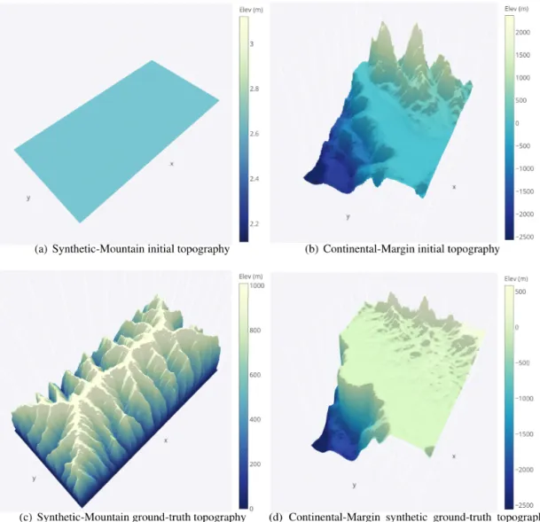
Figure 2.Synthetic-Mountain: initial and eroded ground-truth topography after a million years of evolution. Continental-Margin: initial and eroded ground-truth topography and sediment after 1 million years. The erosion–deposition that forms sediment deposition after 1 million years is also shown. Note thatxaxis represents the latitude;yaxis represents the longitude, and that aligns with Fig. 1a. The elevation in metres (m) is given by thezaxis, which is further shown as a colour bar. The Synthetic-Mountain problem does not align with actual landscape.
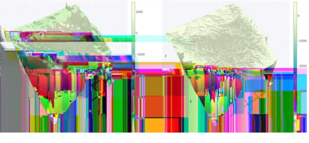
Figure 3.Tasmania: initial and eroded ground-truth topography along with erosion–deposition that shows sediment deposition after 1 million years evolution. Note thatxaxis represents the latitude;yaxis represents the longitude, and that aligns with Fig. 1b for the Tasmania problem. The elevation in metres (m) is given by thezaxis, which is further shown as a colour bar.
along the eastern margin of Te Waipounamu/South Island of Aotearoa/New Zealand as shown in Fig. 1a. We use Badlands to evolve the initial landscape with parameter settings given in Tables 1 and 2 and create the respective problems synthetic ground-truth topography.
The initial and synthetic ground-truth topographies along with erosion/deposition for these problems appear in Figs. 2 and 3, respectively. Note that the figure shows that the
Synthetic-Mountain is flat in the beginning, then given a con-stant uplift rate, along with weathering with concon-stant pre-cipitation rate, which creates the mountain topography. We use present-day topography as the initial topography in the Continental-Margin and Tasmania problems, whereas we use a synthetic flat region for Synthetic-Mountain initial topogra-phy. The problems involve an erosion–deposition model his-tory that is used to generate synthetic ground-truth data for
Table 2.True values of parameters.
Rainfall Uplift
Topography (m a−1) Erod. nvalue mvalue Marine Surface (mm a−1)
Continental-Margin 1.5 5.0×10⁻⁶ 1.0 0.5 0.5 0.8 –
Synthetic-Mountain 1.5 5.0×10⁻⁶ 1.0 0.5 – – 1.0
Tasmania 1.5 5.0×10⁻⁶ 1.0 0.5 0.5 0.8 –
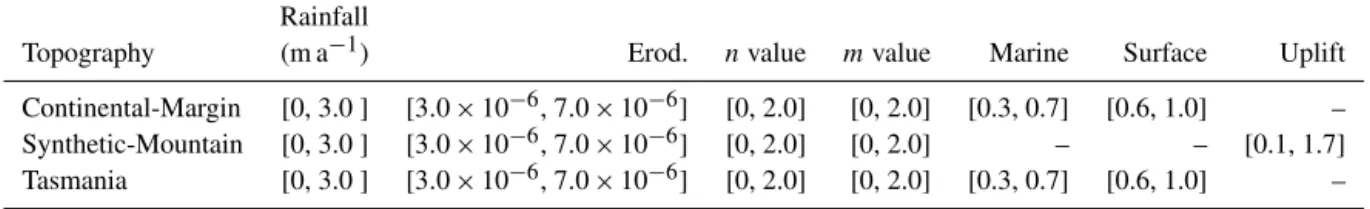
Table 3.Prior distribution range of model parameters. Rainfall
Topography (m a−1) Erod. nvalue mvalue Marine Surface Uplift
Continental-Margin [0, 3.0 ] [3.0×10⁻⁶, 7.0×10⁻⁶] [0, 2.0] [0, 2.0] [0.3, 0.7] [0.6, 1.0] – Synthetic-Mountain [0, 3.0 ] [3.0×10⁻⁶, 7.0×10⁻⁶] [0, 2.0] [0, 2.0] – – [0.1, 1.7]
Tasmania [0, 3.0 ] [3.0×10⁻⁶, 7.0×10⁻⁶] [0, 2.0] [0, 2.0] [0.3, 0.7] [0.6, 1.0] –
the final model state that we then attempt to recover. Hence, the likelihood function given in the following subsection takes both the landscape topography and erosion–deposition ground truth into account. The Continental-Margin and Tas-mania cases feature six free parameters (Table 2), whereas the Synthetic-Mountain features five free parameters. Note that the marine diffusion coefficients are absent for the Synthetic-Mountain problem since the region does not cover or overlap with coastal and marine areas. The main reason behind choosing the two benchmark problems is due to their nature, i.e. the Synthetic-Mountain problem features uplift rate, which is not present in the Continental-Margin prob-lem. The Continental-Margin problem features other param-eters such as the marine coefficients. The Tasmania problem features a much bigger region; hence, it takes more compu-tational time for running a single model. The common fea-ture in all three problems is that they model both the ele-vation and erosion/deposition topography. Furthermore, we draw the priors from a uniform distribution with a lower and upper limit given in Table 3.
3.2 Bayeslands likelihood function
The Bayeslands likelihood function evaluates Badlands to-pography simulation along with the successive erosion– deposition, which denotes the sediment thickness evolution through time. More specifically, the likelihood function eval-uates the effect of the proposals by taking into account the difference between the final simulated Badlands topogra-phy and the ground-truth topogratopogra-phy. The likelihood func-tion also considers the difference between the simulated and ground-truth sediment thickness at selected time intervals, which has been adapted from previous work (Chandra et al., 2019c) and is given as follows. The initial topography is de-noted by D0 with D0=(D0,s1. . ., D0,sn), where si
corre-sponds to sitesi, with the coordinates given by the latitude ui and longitude vi.
We assume an inverse gamma (IG) prior τ2∼ IG(ν/2,2/ν) and integrate it so that the likelihood for the topography at timet=T is
Ll(θ)∝ n Y i=1 1+ Dsi,T−fsi,T(θ) 2 ν !−ν+12 , (1)
whereνis the number of observations, and the subscript “l” inLl(θ)denotes that it is the landscape likelihood to distin-guish it from a sediment likelihood.
Although Badlands produces successive time-dependent topographies, only the final topographyDT is used for the calculation of the elevation likelihood since little ground-truth information is available for the detailed evolution of surface topography. In contrast, the time-dependence of sedimentation can be used to ground-truth the time-dependent evolution of surface process models that include sediment transportation and deposition. The sediment ero-sion/deposition values at time (zt) are simulated (predicted) by the Badlands model given set of parameters,θ, plus some Gaussian noise as follows:
zsj,t=gsj,t(θ)+ηsj,t with ηsj,t∼(0, χ
2). (2)
The sediment likelihoodLs(θ), after integrating outχ2, be-comes Ls(θ)∝ T Y t=1 J Y j=1 1+(zsj,t −gsj,t(θ)) 2 ν !−ν+12 . (3)
The combined likelihood takes both elevation and sedi-ment/deposition into account
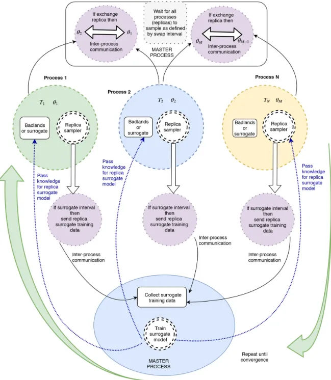
Figure 4.Surrogate-assisted Bayeslands using the parallel tempering MCMC framework. We carry out the training in the master (manager) process, which features the global surrogate model. The replica processes provide the surrogate training dataset to the master process using inter-process communication. We employ a neural network model for the surrogate model. After training, we transfer the knowledge (neural network weights) to each of the replicas to enable estimation of pseudo-likelihood. Refer to Algorithm 1 for further details.
Note that although we used the log-likelihood version in our actual implementation, we refer to it as the likelihood throughout the paper.
3.3 Surrogate-assisted Bayeslands
The surrogate model learns from the relationship between the set of input parameters and the response given by the true
(Badlands) model. The input is the set of proposals by the respective replica samplers in the parallel tempering MCMC sampling algorithm. We refer to the likelihood estimation by the surrogate model as thepseudo-likelihood.
We need to take into account the cost of inter-process munication in parallel computing environment to avoid com-putational overhead. As given in our previous
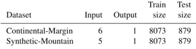
implementa-Table 4.Neural network architecture for the different problems. Train Test
Dataset Input Output size size
Continental-Margin 6 1 8073 879
Synthetic-Mountain 5 1 8073 879
tion (Chandra et al., 2019c), theswap intervalrefers to the number of iterations after which each replica pauses and can undergo a replica transition. After the swap proposal is ac-cepted or rejected, the respective replica sampling is resumed while undergoing Metropolis transition in between the swap intervals. We incorporate the surrogate-assisted estimation into the multicore parallel tempering algorithm. Our previous work (Chandra et al., 2020) used asurrogate intervalthat de-termines the frequency of training by collecting the history of past samples with their likelihood from the respective repli-cas. We need a swap interval of several samples when dealing with small-scale models that take a few seconds to run; how-ever for large models, we recommend having a swap interval of 1.
Taking into account that the true model is represented as y=f (x), the surrogate model provides an approximation in the formyˆ= ˆf (x); such thaty= ˆy+e, whereerepresents the difference or error. The task of the surrogate model is to provide an estimate for the pseudo-likelihood by training from the history of proposals, which is given by the set of inputxr,sand likelihoodys, where “s” represents the sample and “r” represents the replica. Hence, we create the training dataset 8for the surrogate by fusion ofxr,s across all the replica for a given surrogate intervalψ, which can be formu-lated as follows:
8=(x1,s, . . .,x1,s+ψ, . . .,xM,s, . . .,xM,s+ψ)
λ=(y1,s, . . ., y1,s+ψ, . . ., yM,s, . . ., yM,s+ψ), (5) where,xr,srepresents the set of parameters proposed at sam-ple “s”,yr,s=log p(y|xr,s)
is the likelihood, which is de-pendent on data and the Badlands model, andMis the total number of replicas.2denotes the training surrogate dataset, which features input 8and responseλat the end of every surrogate interval denoted bys+ψ. Therefore, we give the pseudo likelihood as yˆ= ˆf (2), where fˆ is the prediction from the surrogate model. The likelihood in training data is altered, with respect of the temperature, since it has been changed by takingLlocal/Trfor given replica “r”. We undo this change by multiplying the likelihood by the respective replica temperature level taken from the geometric tempera-ture ladder.
We present surrogate-assisted Bayeslands in Algorithm 1, which features parallel processing of the ensemble of repli-cas. The highlighted region in the colour pink of the Algo-rithm 1 shows different processing cores running in parallel, shown in Fig. 4 where the manager process is highlighted.
Due to multiple parallel processing replicas, it is not straight-forward to implement when to terminate sampling. Hence, the termination condition waits for all the replica processes to end as it monitors the number of active oralive replica pro-cessesin the manager process. We begin by setting the num-ber of alive replicas in the ensemble (alive=M) and then the replicas that sampleθn are assigned values using a uniform distribution[−α, α]; whereαdefines the range of the respec-tive parameters. We then assign the user-defined parameters, which include the number of replica samplesRmax, swap-intervalRswap, surrogate interval,ψ, and surrogate probabil-itySprob, which determines the frequency of employing the surrogate model for estimating the pseudo-likelihood.
The samples that cover the first surrogate interval makes up the initial surrogate training data2, which feature all the replicas. We then train the surrogate to estimate the pseudo-likelihood when required according to the surrogate proba-bility. Figure 4 shows how the manager processing unit con-trols the respective replicas, which samples for the given sur-rogate interval. Then, the algorithm calculates the replica transition probability for the possibility of swapping the neighbouring replicas. The information flows from replica process to manager process usingsignal()via inter-process communication given by the replica process as shown in Stage 2.2, 3.1, and 4.0 of Algorithm 1, and further shown in Fig. 4.
To enable better estimation for the pseudo-likelihood, we retrain the surrogate model for remaining surrogate interval blocks until the maximum time (Rmax). We train the surro-gate model only in the manager process and the algorithm passes the surrogate model copy with the trained parameters to the ensemble of replica processes for predicting or estimat-ing the pseudo-likelihood. The samples associated with the true-likelihood only becomes part of the surrogate training dataset. In Stage 1.4 of Algorithm 1, the pseudo-likelihood (Lsurrogate) provides an estimation with given proposal θs∗. Stage 1.5 calculates the likelihood moving average of past three likelihood values,Lpast = mean(Ls−1, Ls−1, Ls−2). In Stage 1.6, we combine the moving average likelihood with the pseudo-likelihood to give a prediction that considers the present replica proposal and taking into account the past, Llocal=(0.5×Lsurrogate)+0.5×Lpast. The surrogate train-ing can consume a significant portion of time, which is de-pendent on the size of the problem in terms of the number of parameters and also the type of surrogate model used, along with the training algorithm. We evaluate the trade-off be-tween quality of estimation by pseudo-likelihood and over-all cost of computation for the true likelihood function for different types of problems.
We validate the quality of estimation from the surrogate model by the root-mean-squared error (RMSE), which con-siders the difference between the true likelihood and the pseudo-likelihood. This can be seen as a regression prob-lem with multi-input (parameters) and a single output
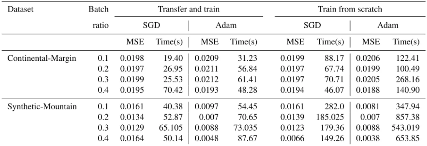
(like-Table 5.Evaluation of surrogate training accuracy.
Dataset Batch Transfer and train Train from scratch
ratio SGD Adam SGD Adam
MSE Time(s) MSE Time(s) MSE Time(s) MSE Time(s)
Continental-Margin 0.1 0.0198 19.40 0.0209 31.23 0.0199 88.17 0.0206 122.41 0.2 0.0197 26.95 0.0211 56.84 0.0197 67.74 0.0199 100.49 0.3 0.0199 25.53 0.0212 61.41 0.0197 70.71 0.0205 268.16 0.4 0.0195 70.42 0.0193 48.28 0.0194 46.07 0.0188 140.90 Synthetic-Mountain 0.1 0.0161 40.38 0.0097 54.45 0.0161 282.0 0.0081 347.94 0.2 0.0134 52.87 0.007 70.65 0.0139 185.025 0.007 857.38 0.3 0.0129 65.105 0.0088 73.035 0.0123 179.36 0.0088 543.019 0.4 0.0164 50.14 0.0048 87.67 0.0066 149.26 0.0038 653.85
Table 6.Convergence diagnosis (PSRF score) for Continental-Margin problem.
Mean
Proposal Method Precip. Erod. mvalue nvalue c-marine c-surface R score
RW PT-Bayeslands 1.50 1.6 1.14 4.82 2.62 1.56 2.21
ARW PT-Bayeslands 1.26 1.55 1.26 1.63 1.38 1.13 1.37
RW SAPT-Bayeslands 4.06 1.70 6.57 1.51 1.46 1.49 2.80
ARW SAPT-Bayeslands 1.33 2.88 1.22 2.46 1.03 1.30 1.70
lihood). Hence, we report the surrogate prediction quality by
RMSEsur= v u u t 1 N N X i=1 yi− ˆyi2,
where yi and yˆi are the true likelihood and the pseudo-likelihood values, respectively.N is the number of cases the surrogate has used during sampling.
We further note that the framework uses parallel tempering MCMC in the first stage of sampling and then transforms into the second stage where the temperature ladder is changed such thatTi =1, for all replicas,i=1, 2, ...,M. This strat-egy enables exploration in the first stage and exploitation in the second stage. We combine the respective replica poste-rior distributions once the termination condition is met and show their mean and standard deviation of the prediction in the results.
We evaluate the prediction performance by comparing the predicted/simulated Badlands landscape with the ground-truth data using the root-mean-squared error (RMSE). We compute the RMSE for the elevation (elev) and sediment erosion/deposition (sed) at each iteration of the sampling
scheme using RMSEelev= v u u t 1 n×m n X i=1 n X j=1 gθˆT ,i,j −gT ,i,j(θ ) 2 RMSEsed= v u u t 1 nt×v nt X t=1 m X j=1 fθˆt,j −f θt,j 2 ,
whereθˆis an estimated value of θ, andθ is the true value representing the synthetic ground truth.f (.)andg(.) repre-sent the outputs of the Badlands model, whilemandn rep-resent the size of the selected topography.v is the number of selected points from sediment erosion/deposition over the selected time frame,nt.
3.4 Surrogate model
To choose a particular surrogate model, we need to con-sider the computational resources for training the model dur-ing the sampldur-ing process. The literature review showed that Gaussian process models, neural networks, and radial basis functions (Broomhead and Lowe, 1988) are popular choices for surrogate models. We note that Badlands LEM features about a dozen free parameters in one of the simplest cases; this increases when taking into account spatial and temporal dependencies. For instance, the precipitation rate for a mil-lion years can be represented by a single parameter or by 10 different parameters that capture every 100 000 years for 10
Table 7.Evaluation for Continental-Margin problem.
Method Sprob ψ RMSEelev RMSEelev RMSEsed RMSEsed Time (s)
(mean) (SD) (mean) (SD)
PT-Bayeslands N/A N/A 78.80 10.03 35.91 11.36 3243.30
SAPT-Bayeslands 0.20 0.05 75.53 9.89 35.68 10.93 3082.53 SAPT-Bayeslands 0.40 0.05 80.22 15.63 44.72 16.52 2450.77 SAPT-Bayeslands 0.60 0.05 82.04 8.23 44.33 13.37 1859.52 SAPT-Bayeslands 0.80 0.05 79.30 26.70 43.29 18.68 1149.63 SAPT-Bayeslands 0.20 0.10 76.92 11.59 48.19 11.46 3075.31 SAPT-Bayeslands 0.40 0.10 82.43 11.58 46.47 12.55 2494.13 SAPT-Bayeslands 0.60 0.10 80.12 12.08 47.80 19.05 1934.34 SAPT-Bayeslands 0.80 0.10 88.81 20.61 51.12 14.26 1148.80 SAPT-Bayeslands 0.20 0.15 44.90 33.54 23.95 19.86 2914.06 SAPT-Bayeslands 0.40 0.15 73.64 8.05 38.53 10.02 2495.56 SAPT-Bayeslands 0.60 0.15 83.38 8.45 51.15 19.07 1986.51 SAPT-Bayeslands 0.80 0.15 84.73 10.04 39.78 14.44 1294.64
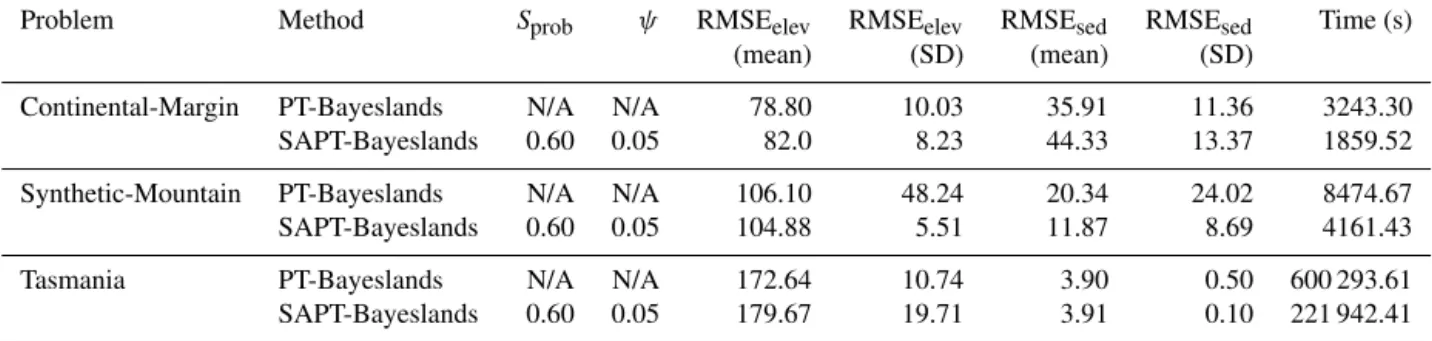
Table 8.Performance comparison for respective problems and methods. N/A: not applicable.
Problem Method Sprob ψ RMSEelev RMSEelev RMSEsed RMSEsed Time (s)
(mean) (SD) (mean) (SD)
Continental-Margin PT-Bayeslands N/A N/A 78.80 10.03 35.91 11.36 3243.30
SAPT-Bayeslands 0.60 0.05 82.0 8.23 44.33 13.37 1859.52
Synthetic-Mountain PT-Bayeslands N/A N/A 106.10 48.24 20.34 24.02 8474.67
SAPT-Bayeslands 0.60 0.05 104.88 5.51 11.87 8.69 4161.43
Tasmania PT-Bayeslands N/A N/A 172.64 10.74 3.90 0.50 600 293.61
SAPT-Bayeslands 0.60 0.05 179.67 19.71 3.91 0.10 221 942.41
different regions, which can account for 1000 parameters in-stead of 1. Considering hundreds or thousands of unknown Badlands model parameters, the surrogate model needs to be efficiently trained without taking lots of computational resources. The flexibility of the model to have incremental training is also needed, and hence, we rule out Gaussian pro-cess models since they have limitations in training when the size of the dataset increases to a certain level (Rasmussen, 2004). Therefore, we use neural networks as the choice of the surrogate model, and the training data and neural network model is formulated as follows.
We denote the surrogate model training data by8andλ, which is shown in Eq. (5), where8is the input, andλis the desired output of the model. The prediction of the model is denoted by λˆ. We use a feedforward neural network as the surrogate model. Given inputxt,f (xt)is computed by the feedforward neural network with one hidden layer defined by the function f (xt)=g δo+ H X h=1 vjg δh+ I X d=1 wdhxt , (6)
whereδo andδh are the bias weights for the output o and hiddenhlayer, respectively.vjis the weight which maps the hidden layerhto the output layer.wdh is the weight which mapsxt to the hidden layerh, andg(.)is the activation func-tion for the hidden and output layer units. We use ReLU (rectified linear unitary function) as the activation function. The learning or optimization task then is to iteratively update the weights and biases to minimize the cross-entropy loss J (W,b). This can be done using gradient update of weights using the Adam (adaptive moment estimation) learning algo-rithm (Kingma and Ba, 2014) and stochastic gradient descent (Bottou, 1991, 2010). We experimentally evaluate them for training the feedforward network for the surrogate model in the next section.
3.5 Proposal distribution
Bayeslands features random-walk (RW) and adaptive-random-walk (ARW) proposal distributions which will be evaluated further for surrogate-assisted Bayeslands in our experiments. In our previous work (Chandra et al., 2019a), ARW showed better convergence properties when
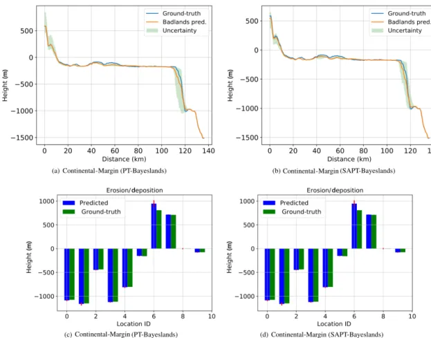
com-Figure 5.Topography cross section and erosion–deposition prediction for 10 chosen points (selected coordinates denoted by location iden-tifier, ID, number) for Continental-Margin problem from results summarized in Table 8.
pared to RW proposal distribution. The RW proposal dis-tribution features 6 as the diagonal matrix, so that 6= diag(σ12, . . ., σP2), whereσjis the step size of thejth element of the parameter vectorθ. The step size forθj is a combina-tion of a fixed step sizeφ, which is common to all parame-ters, multiplied by the range of possible values for parameter θj; henceσj =(aj−bj)×φ, whereaj andbjrepresent the maximum and minimum limits of the prior for θj given in Table 2. In our experiments, the RW proposal distribution employs fixed step size,φ=0.05,
The ARW proposal distribution features adaptation of the diagonal matrix 6 at every K interval of within-replica sampling. It allows for the dependency between elements of θ and adapts during sampling (Haario et al., 2001). We adapt the elements of 6 for the posterior distribution us-ing the sample covariance of the current chain history 6= cov({θ[0], . . .,θ[i−1]})+diag(λ21, . . ., λ2P), whereθ[i]is theith iterate ofθin the chain, andλjis the minimum allowed step sizes for each parameterθj.
3.6 Design of experiments
We demonstrate effectiveness of surrogate-assisted parallel tempering (SAPT-Bayeslands) framework for selected
Bad-lands LEMs taken from our previous study (Chandra et al., 2019c).
We first investigate the effects of different surrogate training procedures and parameter evaluation for SAPT-Bayeslands using smaller synthetic problems. Afterwards, we apply the methodology to a larger landscape evolution problem, which is Tasmania, Australia. We design the exper-iments as follows.
1. We generate a dataset for training and testing the sur-rogate for the Synthetic-Mountain and Continental-Margin landscape evolution problems. We use the neu-ral network model for the surrogate and evaluate differ-ent training techniques.
2. We evaluate if the transfer of knowledge from previous surrogate interval is better than no transfer of knowledge for Synthetic-Mountain and Continental-Margin prob-lems. Note this is done only with the data generated from the previous step.
3. We provide convergence diagnosis for the RW and ARW proposal distributions in PT-Bayeslands and SAPT-Bayeslands.
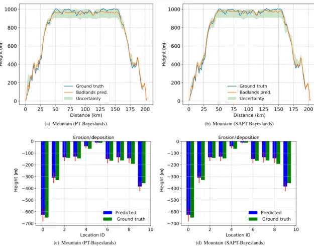
Figure 6.Topography cross section and erosion–deposition prediction for 10 chosen points (selected coordinates denoted by location iden-tifier (ID) number) for Synthetic-Mountain problem from results summarized in Table 8.
4. We integrate the surrogate model into Bayeslands and evaluate the effectiveness of the surrogate in terms of es-timation of the likelihood and computational time. Due to the computational requirements, we only consider the Continental-Margin problem.
5. We then apply SAPT-Bayeslands to all the given prob-lems and compare with PT-Bayeslands.
We use Keras neural networks library (Gulli and Pal, 2017) for implementation of the surrogate. We provide the open-source software package that implements Algorithm 1 along with benchmark problems and experimental results1.
We use a geometric temperature ladder with a maximum temperature of Tmax=2 for determining the temperature level for each of the replicas. In trial experiments, the se-lection of these parameters depended on the performance in terms of the number of accepted samples and prediction ac-curacy of elevation and sediment/deposition. We use replica-exchange or swap interval value;Rswap=3 samples that de-termine when to check whether to swap with the neighbour-ing replica. In previous work (Chandra et al., 2019c), we 1Surrogate-assisted Bayeslands: https://github.com/
intelligentEarth/surrogateBayeslands, last access: 6 July 2020
observed that increasing the number of replicas up to a cer-tain point does not necessarily mean that we get better per-formance in terms of the computational time or prediction accuracy. In this work, we limit the number of replicas to Rnum=8 for all experiments with maximum of 5000 sam-ples.
We use a 50 % burn in, which discards the portion of sam-ples in the parallel tempering MCMC stage as done in our previous work (Chandra et al., 2019a).
4 Results
4.1 Surrogate accuracy
To implement the surrogate model, we need to evaluate the training algorithm, such as Adam and stochastic gradient de-scent (SGD). Furthermore, we also evaluate specific param-eters, such as the size of the surrogate interval (batch ratio), the neural network topology for the surrogate, and the effec-tiveness of either training from scratch or utilizing previous knowledge for surrogate training (transfer and train). We cre-ate a training dataset from the cases where the true likelihood was used, which compromises the history of the set of
pa-Figure 7.Topography cross section and erosion–deposition prediction for 10 chosen points (selected coordinates denoted by location iden-tifier, ID, number) for Tasmania problem from results summarized in Table 8.
Figure 8. Surrogate likelihood vs. true likelihood estimation for Continental-Margin problem (RMSEsur=3605).
Figure 9.Surrogate likelihood vs. true likelihood estimation for Synthetic-Mountain problem (RMSEsur=9917).
rameters proposed with the corresponding likelihood. This is done for standalone evaluation of the surrogate model, which further ensures that the experiments are reproducible since different experimental runs create different datasets depend-ing on the exploration durdepend-ing sampldepend-ing. We then evaluate the neural network model designated for the surrogate using two major training algorithms which featured the Adam op-timizer and stochastic gradient descent. The parameters that define the neural network surrogate model used for the ex-periments are given in Table 4. Note that the train size in Table 4 refers to the maximum size of the dataset. The train-ing is done in batches where the batch ratio determines the training dataset size, as shown in Table 5.
Table 5 presents the results for the experiments that took account of the training data collected during sam-pling for two benchmark problems (Continental-Margin and Synthetic-Mountain). Note that we report the mean value of the mean-squared-error (MSE) for the given batch ra-tio from 10 experiments. The batch rara-tio is taken, in rela-tion to the maximum number of samples across the chains (Rmax/Rnum). We normalize the likelihood values (out-comes) in the dataset to the range [0,1]. In most cases, the ac-curacy of the neural network is slightly better when training from scratch with combined data; however, there is a consid-erable trade-off with the time required to train the network. The results show that the transfer and train methodology, in general, requires much lower computational time when com-pared to training from scratch with combined data. Moreover, in comparison to SGD and Adam training algorithms, we ob-serve that SGD achieves slightly better accuracy than Adam for Continental-Margin problem. However, Adam, having an adaptive learning rate, outperforms SGD in terms of the time required to train the network. Thus, we can summarize that transfer and train method is better since it saves significant computation time with a minor trade-off with accuracy. 4.2 Convergence diagnosis
The Gelman–Rubin diagnostic (Gelman and Rubin, 1992) is one of the popular methods used for evaluating con-vergence by analysing the behaviour of multiple Markov chains. The assessment is done by comparing the estimated between-chain and within-chain variances for each parame-ter, where large differences between the variances indicate non-convergence. The diagnosis reports the potential scale reduction factor (PSRF), which gives the ratio of the current variance in the posterior variance for each parameter com-pared to that being sampled, and the values for the PSRF near 1 indicates convergence. We analyse five experiments for each case using different initial values for 5000 samples for each problem configuration.
Table 6 presents the convergence diagnosis using the PSRF score for RW and ARW proposal distributions for PT-Bayeslands and SAPT-PT-Bayeslands. We notice that ARW has a lower PSRF score (mean) when compared to the RW
pro-posal distribution, which indicates better convergence. We also notice that the ARW SAPT-Bayeslands maintains con-vergence with a PSRF score close to ARW PT-Bayeslands when compared to rest of the configurations. This suggests that although we use surrogates, convergence can be main-tained up to a certain level, which is better than RW PT-Bayeslands.
4.3 Surrogate-assisted Bayeslands
We investigate the effect of the surrogate probability (Sprob) and surrogate interval (ψ) on the prediction accuracy (RMSEelevand RMSEsed) and computational time. Note that we report the prediction accuracy mean and standard de-viation (mean and SD) of accepted samples over the sam-pling time after removing the burn-out period. We report the computational time in seconds (s). Table 7 presents the performance of the respective methods (PT-Bayeslands and SAPT-Bayeslands) with respective parameter settings for the Continental-Margin problem. In SAPT-Bayeslands, we ob-serve that there is not a major difference in the accuracy of el-evation or erosion/deposition given different values ofSprob. Nevertheless, there is a significant difference in terms of the computational time where higher values ofSprob save com-putational time. Furthermore, we notice that there is not a significant difference in the prediction accuracy given differ-ent values ofψ, which suggests that the selected values are sufficient.
We select a suitable combination of the set of parame-ters evaluated in the previous experiment (Sprob=0.6 and ψ=0.05) and apply them to rest of the problems. Table 8 gives a comparison of performance for Continental-Margin and Synthetic-Mountain problems, along with the Tasma-nia one, which is a bigger and more computationally ex-pensive problem. We notice that the performance of SAPT-Bayeslands is similar to PT-SAPT-Bayeslands, while a significant portion of computational time is saved.
Figures 5, 6, and 7 provide a visualization of the elevation prediction accuracy when compared to actual ground truth between the given methods from results given in Table 8. We also provide the prediction accuracy of erosion/deposition for 10 chosen points taken at selected locations. Although both methods provide erosion/deposition prediction for four successive time intervals, we only show the final time inter-val. In both the Continental-Margin and Synthetic-Mountain problems, we notice that the prediction accuracy of PT-Bayeslands is very similar to SAPT-PT-Bayeslands, and the Bad-lands prediction of the topography is close to ground truth, within the credible interval. This indicates that the use of sur-rogates has been beneficial where no major loss in accuracy in prediction is given. In the case of the Tasmania problem, there is a loss in Badlands prediction accuracy, which could be due to the size of the problem. Nevertheless, this loss is not that clear from results in Table 8. It could be that the
topog-raphy prediction is mostly inconsistent at the cross section where it features mountainous regions.
Figures 8 and 9 show the true likelihood and prediction by the surrogate for the Continental-Margin and Synthetic-Mountain problems, respectively. We notice that at certain intervals given in Fig. 8, given by different replica, there is inconsistency in the predictions. Moreover, Fig. 9 shows that the log-likelihood is very chaotic, and hence there is diffi-culty in providing robust prediction at certain points in the time given by samples for the respective replica.
4.4 Discussion
We observe that the surrogate probability is directly related to the computational performance; this is obvious since com-putational time depends on how often we use the surrogate. Our concern is the prediction performance, especially while increasing the use of the surrogate as it could lower the ac-curacy, which can result in a poor estimation of the param-eters. According to the results, the accuracy is well retained given a higher probability of using surrogates. In the cross section presented in the results for Continental-Margin and Synthetic-Mountain problems, we find that there is not much difference in the accuracy given in prediction by the SAPT-Bayeslands when compared to PT-SAPT-Bayeslands. Moreover, in the application to a more computationally intensive prob-lem (Tasmania), we find that a significant reduction in com-putational time is achieved. Although we demonstrated the method using small-scale models that run within a few sec-onds to minutes, the computational costs of continental-scale Badlands models are extensive. For instance, the computa-tional time for a 5 km resolution for the Australian continent Badlands model for 149 million years is about 72 h; hence, in the case when thousands of samples are required, the use of surrogates can be beneficial. We note that improved ef-ficiency of the surrogate-assisted Bayeslands comes at the cost of accuracy for some problems (in case of the Tasma-nia problem), and there is a trade-off between accuracy and computational time.
In future work, rather than a global surrogate model, we could use the local surrogate model on its own, where the training only takes place in the local surrogates by relying on the history of the likelihood and hence taking a univariate time series prediction approach using neural networks. Our primary contribution is in terms of the parallel-computing-based open-source software and the proposed underlying framework for incorporating surrogates, taking into account complex issues such as inter-process communication. This opens the road to using different types of surrogate models while using the underlying framework and open-source soft-ware. Given that the sediment erosion/deposition is temporal, other ways of formulating the likelihood could be possible; for instance, we could have a hierarchical Bayesian model with two stages for MCMC sampling (Chib and Carlin, 1999; Wikle et al., 1998).
The initial evaluation for the setup surrogate model shows that it is best to use a transfer learning approach where the knowledge from the past surrogate interval is utilized and refined with new surrogate data. This consumes much less time than accumulating data and training the surrogate from scratch at every surrogate interval. We note that in the case when we use the surrogate model for pseudo-likelihood, there is no prediction given by the surrogate model. The pre-diction (elevation topography and erosion–deposition) dur-ing sampldur-ing are gathered only from the true Badlands model evaluation rather than the surrogate. In this way, one could argue that the surrogate model is not mimicking the true model; however, we are guiding the sampling algorithm to-wards forming better proposals without evaluation of the true model. A direction forward is in incorporating other forms of surrogates, such as running a low-resolution Badlands model as the surrogate, which would be computationally faster in evaluating the proposals; however, limitations in terms of the effect of resolution setting on Badlands topography simula-tion may exist.
Furthermore, computationally efficient implementations of landscape evolution models that only feature landscape evolution (Braun and Willett, 2013) could be used as the surrogate, while we could use Badlands model that fea-tures both landscape evolution and erosion/deposition as the true model. We could also use computationally efficient im-plementations of landscape evolution models that consider parallel processing (Hassan et al., 2018) in the Bayeslands framework. In this case, the challenge would be in allocat-ing specialized processallocat-ing cores for Badlands and others for parallel tempering MCMC.
We adapted the surrogate framework developed for ma-chine learning (Chandra et al., 2020) with a different pro-posal distribution instead of using gradient-based propro-posals. Gradient-based parameter estimation has been very popular in machine learning due to availability of gradient informa-tion. Due to the complexity in geological or geophysical nu-merical forward models, it is challenging to obtain gradients, which has been the case for the Badlands landscape evo-lution model. We used random-walk and adaptive-random-walk proposal distributions which have limitations; hence, we need to incorporate advanced meta-heuristic techniques to form non-gradient-based proposals for efficient search. Our study is limited to a relatively small set of free param-eters, and a significant challenge would be to develop surro-gate models with an increased set of parameters.
5 Conclusions
We presented a novel application of surrogate-assisted par-allel tempering that features parpar-allel computing for land-scape evolution models using Badlands. Initially, we exper-imented with two different approaches for training the sur-rogate model, where we found that a transfer learning-based
approach is beneficial and could help reduce the computa-tional time of the surrogate. Using this approach, we pre-sented the experiments that featured evaluating certain key parameters of the surrogate-based framework. In general, we observed that the proposed framework lowers the computa-tional time significantly while maintaining the required qual-ity in parameter estimation and uncertainty quantification.
In future work, we envision applying the proposed frame-work to more complex applications such as the evolution of continental-scale landscapes and basins over millions of years. We could use the approach for other forward mod-els such as those that feature geological reef development or lithospheric deformation. Furthermore, the posterior dis-tribution of our parameters requires multimodal sampling methods; hence, a combination of meta-heuristics for pro-posals with surrogate-assisted parallel tempering could im-prove exploration features and also help in lowering the com-putational costs.
Appendix A: Parallel tempering MCMC
Parallel tempering MCMC features massive parallelism with enhanced exploration capabilities. It features several replicas with slight variations in the acceptance criteria through re-laxation of the likelihood with a temperature ladder that af-fects the replica sampling acceptance criterion. The replicas associated with higher temperature levels have more chance in accepting weaker proposals, which could help in escap-ing a local minimum. Given an ensemble of Mreplicas de-fined by a temperature ladder, we define the state by X= x1, x2, . . ., xM, wherexiis the replica at temperature levelTi. We construct a Markov chain to sample proposalxiand eval-uate it using the likelihoodL(xi)for each replica defined by temperature levelTi. At each iteration, the Markov chain can feature two types of transitions that include the Metropolis transitionand thereplica transition.
In the Metropolis transition phase, we independently sam-ple each replica to perform localMonte Carlomoves as de-fined by the temperature ladder for the replica by relaxing or changing the likelihood in relation to the temperature level L(xi)/Ti. We sample configurationxi∗from a proposal dis-tributionqi(.|xi). TheMetropolis–Hastingsratio at tempera-ture levelTiis given by
Llocal xi→xi∗ = exp −1 Ti L xi∗− L (xi) , (A1)
whereLrepresents the likelihood at the local replica. We ac-cept the new state with probability, min 1, Llocal xi→x∗i. The detailed balance condition holds for each MCMC replica; therefore, it holds for the ensemble system (Calder-head, 2014).
In the replica transition phase, we consider the exchange of the current state between two neighbouring replicas based on the Metropolis–Hastings acceptance criteria. Hence, given a probabilityα, we exchange a pair of replica defined by two neighbouring temperature levels,TiandTi+1.
xi↔xi+1 (A2)
The exchange of neighbouring replicas provides an effi-cient balance between local and global exploration (Sam-bridge, 2013). The temperature ladder and replica exchange have been of the focus of investigation in the past (Calvo, 2005; Liu et al., 2005; Bittner et al., 2008; Patriksson and van der Spoel, 2008), and there is a consensus that they need to be tailored for different types of problems given by their likelihood landscape. In this paper, the selection of tempera-ture spacing between the replicas is carried out using a geo-metric spacing methodology (Vousden et al., 2015), given as follows:
Ti=T(i
−1)/(M−1)
max , (A3)
where i=1, . . ., M and Tmax is maximum temperature, which is user defined and dependent on the problem.
A1 Training the neural network surrogate model We note that stochastic gradient descent maintains a single learning rate for all weight updates, and typically the learn-ing rate does not change durlearn-ing the trainlearn-ing. Adam (adap-tive moment estimation) learning algorithm (Kingma and Ba, 2014) differs from classical stochastic gradient descent, as the learning rate is maintained for each network weight and separately adapted as learning unfolds. Adam computes in-dividual adaptive learning rates for different parameters from estimates of first and second moments of the gradients. Adam features the strengths ofroot mean square propagation (RM-Sprop) andadaptive gradient algorithm(AdaGrad) (Kingma and Ba, 2014; Duchi et al., 2011). Adam has shown bet-ter results when compared to stochastic gradient descent, RMSprop, and AdaGrad. Hence, we consider Adam as the designated algorithm for the neural-network-based surrogate model. We formulate the learning procedure through weight update for iteration numbert for weightsWand biasesbby 2t−1=Wt−1, bt−1 gt = ∇2Jt(2t−1) mt =β1·mt−1+(1−β1)·gt vt=β2·vt−1+(1−β2)·g2t ˆ mt =mt/ 1−β1t ˆ vt=vt/ 1−β2t 2t=2t−1−α.mˆt/ p ˆ vt+ , (A4)
wheremt andvt are the, respectively, first and second mo-ment vectors for iterationt;β1andβ2are constants∈ [0,1]; αis the learning rate, andis a close to zero constant.
Code availability. We provide open-source code along with data and sample results to motivate further work in this area: https://github.com/intelligentEarth/surrogateBayeslands
(last access: 6 July 2020, intelligentEarth, 2020);
https://doi.org/10.5281/zenodo.3892277 (Chandra, 2020).
Author contributions. RC led the project and contributed to writ-ing the paper and designwrit-ing the experiments. DA contributed by running experiments and providing documentation of the results. AK contributed in terms of programming, running experiments, and providing documentation of the results. RDM contributed by man-aging the project, writing the paper, and providing analysis of the results.
Competing interests. The authors declare that they have no conflict of interest.
Acknowledgements. We would like to thank Konark Jain for tech-nical support. R. Dietmar Müller and Danial Azam were supported by the Australian Research Council (grant IH130200012). We sin-cerely thank the reviewers for their comments that helped us in im-proving the paper.
Financial support. This research has been supported by the Univer-sity of Sydney (grant no. SREI Grant 2017-2018) and the Australian Research Council (grant no. IH130200012).
Review statement. This paper was edited by Richard Neale and re-viewed by two anonymous referees.
References
Adams, J. M., Gasparini, N. M., Hobley, D. E. J., Tucker, G. E., Hutton, E. W. H., Nudurupati, S. S., and Istanbulluoglu, E.: The Landlab v1.0 OverlandFlow component: a Python tool for computing shallow-water flow across watersheds, Geosci. Model Dev., 10, 1645–1663, https://doi.org/10.5194/gmd-10-1645-2017, 2017.
Ampomah, W., Balch, R., Will, R., Cather, M., Gunda, D., and Dai, Z.: Co-optimization of CO2EOR and Storage Processes under
Geological Uncertainty, Energy Proc., 114, 6928–6941, 2017. Asher, M. J., Croke, B. F., Jakeman, A. J., and Peeters, L. J.: A
review of surrogate models and their application to groundwater modeling, Water Resour. Res., 51, 5957–5973, 2015.
Bittner, E., Nußbaumer, A., and Janke, W.: Make life
simple: Unleash the full power of the parallel
tem-pering algorithm, Phys. Rev. Lett., 101, 130603,
https://doi.org/10.1103/PhysRevLett.101.130603, 2008. Bottou, L.: Stochastic gradient learning in neural networks, Proc.
Neuro-Nımes, 91, 12, 1991.
Bottou, L.: Large-scale machine learning with stochastic gradi-ent descgradi-ent, in: Proceedings of COMPSTAT’2010, 177–186, Springer, 2010.
Braun, J. and Willett, S. D.: A very efficient O(n), implicit and par-allel method to solve the stream power equation governing flu-vial incision and landscape evolution, Geomorphology, 180–181, 170–179, 2013.
Broomhead, D. S. and Lowe, D.: Radial basis functions, multi-variable functional interpolation and adaptive networks, Tech. rep., Royal Signals and Radar Establishment Malvern (United Kingdom), 1988.
Calderhead, B.: A general construction for parallelizing Metropolis-Hastings algorithms, P. Natl. Acad. Sci. USA, 111, 17408– 17413, 2014.
Calvo, F.: All-exchanges parallel tempering, The J. Chem. Phys., 123, 124106, https://doi.org/10.1063/1.2036969, 2005.
Campforts, B., Schwanghart, W., and Govers, G.: Accurate simu-lation of transient landscape evolution by eliminating numerical diffusion: the TTLEM 1.0 model, Earth Surf. Dynam., 5, 47–66, https://doi.org/10.5194/esurf-5-47-2017, 2017.
Chandra, R.: Surrogate-assisted Bayesian inversion for landscape and basin evolution models (Version 1.0), Geoscientific Model Development, Zenodo, https://doi.org/10.5281/zenodo.3892277, 2020.
Chandra, R., Azam, D., Müller, R. D., Salles, T., and Cripps, S.: BayesLands: A Bayesian inference approach for parameter un-certainty quantification in Badlands, Comput. Geosci., 131, 89– 101, 2019a.
Chandra, R., Jain, K., Deo, R. V., and Cripps, S.: Langevin-gradient parallel tempering for Bayesian neural learning, Neurocomput-ing, 359, 315–326, 2019b.
Chandra, R., Müller, R. D., Azam, D., Deo, R., Butterworth, N., Salles, T., and Cripps, S.: Multi-core parallel tempering Bayeslands for basin and landscape evolution, Geochem. Geo-phys. Geosyst., 20, 5082–5104, 2019c.
Chandra, R., Jain, K., Arpit, K., and Ashray, A.:
Surrogate-assisted parallel tempering for Bayesian
neural learning, Eng. Appl. Art. Intell., 94, 103700, https://doi.org/10.1016/j.engappai.2020.103700, 2020.
Chib, S. and Carlin, B. P.: On MCMC sampling in hierarchical lon-gitudinal models, Stat. Comput., 9, 17–26, 1999.
Díaz-Manríquez, A., Toscano, G., Barron-Zambrano, J. H., and Tello-Leal, E.: A review of surrogate assisted multiobjective evo-lutionary algorithms, Comput. Intel. Neurosc., 2016, 9450460, https://doi.org/10.1155/2016/9420460, 2016.
Duchi, J., Hazan, E., and Singer, Y.: Adaptive subgradient methods for online learning and stochastic optimization, J. Mach. Learn. Res., 12, 2121–2159, 2011.
Gelman, A. and Rubin, D. B.: Inference from iterative simulation using multiple sequences, Stat. Sci., 7, 457–472, 1992.
Geyer, C. J. and Thompson, E. A.: Annealing Markov chain Monte Carlo with applications to ancestral inference, J. Am. Stat. As-soc., 90, 909–920, 1995.
Gulli, A. and Pal, S.: Deep Learning with Keras, Packt Publishing, ISBN 9781787129030, 2017.
Haario, H., Saksman, E., and Tamminen, J.: An adaptive Metropolis algorithm, Bernoulli, 7, 223–242, 2001.
Hassan, R., Gurnis, M., Williams, S. E., and Müller, R. D.: SPGM: A Scalable PaleoGeomorphology Model, SoftwareX, 7, 263– 272, 2018.
Hastings, W. K.: Monte Carlo sampling methods using Markov chains and their applications, Biometrika, 57, 97–109, 1970. Hobley, D. E. J., Sinclair, H. D., Mudd, S. M., and Cowie,
P. A.: Field calibration of sediment flux dependent river incision, J. Geophys. Res.-Earth Surf., 116, F04017, https://doi.org/10.1029/2010JF001935, 2011.
Howard, A. D., Dietrich, W. E., and Seidl, M. A.: Modeling fluvial erosion on regional to continental scales, J. Geophys. Res.-Solid Earth, 99, 13971–13986, 1994.
Hukushima, K. and Nemoto, K.: Exchange Monte Carlo method and application to spin glass simulations, J. Phys. Soc. JPN, 65, 1604–1608, 1996.
intelligentEarth: surrogateBayeslands, available at: https://github. com/intelligentEarth/surrogateBayeslands, last access: 6 July 2020.
Jin, Y.: Surrogate-assisted evolutionary computation: Recent ad-vances and future challenges, Lect. Notes Comput. Sc., 1, 61–70, 2011.
Kass, R. E., Carlin, B. P., Gelman, A., and Neal,
R. M.: Markov chain Monte Carlo in practice: a
roundtable discussion, The Am. Stat., 52, 93–100,
https://doi.org/10.1080/00031305.1998.10480547, 1998. Kingma, D. P. and Ba, J.: Adam: A method for stochastic
optimiza-tion, arXiv preprint arXiv:1412.6980, 2014.
Lamport, L.: On interprocess communication, Distrib. Comput., 1, 86–101, 1986.
Letsinger, J. D., Myers, R. H., and Lentner, M.: Response surface methods for bi-randomization structures, J. Qual. Technol., 28, 381–397, 1996.
Lim, D., Jin, Y., Ong, Y.-S., and Sendhoff, B.: Generalizing surrogate-assisted evolutionary computation, IEEE Trans. Evo-lut. Comput., 14, 329–355, 2010.
Liu, P., Kim, B., Friesner, R. A., and Berne, B. J.: Replica exchange with solute tempering: A method for sampling biological systems in explicit water, P. Natl. Acad. Sci. USA, 102, 13749–13754, 2005.
Marinari, E. and Parisi, G.: Simulated tempering: a new Monte Carlo scheme, EPL (Europhysics Letters), 19, 451–458, 1992. Metropolis, N., Rosenbluth, A. W., Rosenbluth, M. N., Teller, A. H.,
and Teller, E.: Equation of state calculations by fast computing machines, The J. Chem. Phys., 21, 1087–1092, 1953.
Montgomery, D. C. and Vernon M. Bettencourt, J.: Multiple re-sponse surface methods in computer simulation, Simulation, 29, 113–121, 1977.
Navarro, M., Le Maître, O. P., Hoteit, I., George, D. L., Mandli, K. T., and Knio, O. M.: Surrogate-based parameter inference in debris flow model, Comput. Geosci., 22, 1–17, 2018.
Neal, R. M.: Sampling from multimodal distributions using tem-pered transitions, Stat. Comput., 6, 353–366, 1996.
Neal, R. M.: Bayesian learning for neural networks, vol. 118, Springer Science & Business Media, 2012.
Olierook, H. K., Scalzo, R., Kohn, D., Chandra, R., Farahbakhsh, E., Clark, C., Reddy, S. M., and Müller, R. D.: Bayesian geo-logical and geophysical data fusion for the construction and un-certainty quantification of 3D geological models, Geosc. Front., https://doi.org/10.1016/j.gsf.2020.04.015, in press, 2020.
Ong, Y. S., Nair, P. B., and Keane, A. J.: Evolutionary optimization of computationally expensive problems via surrogate modeling, AIAA J., 41, 687–696, 2003.
Ong, Y. S., Nair, P., Keane, A., and Wong, K.: Surrogate-assisted evolutionary optimization frameworks for high-fidelity engineer-ing design problems, in: Knowledge Incorporation in Evolution-ary Computation, 307–331, Springer, 2005.
Pall, J., Chandra, R., Azam, D., Salles, T., Webster, J. M., Scalzo, R., and Cripps, S.: Bayesreef: A Bayesian inference framework for modelling reef growth in response to environmental change and biological dynamics, Environ. Modell. Softw., 125, 104610, https://doi.org/10.1016/j.envsoft.2019.104610, 2020.
Patriksson, A. and van der Spoel, D.: A temperature predictor for parallel tempering simulations, Phys. Chem. Chem. Phys., 10, 2073–2077, 2008.
Rasmussen, C. E.: Gaussian processes in machine learning, in: Ad-vanced lectures on machine learning, 63–71, Springer, 2004. Razavi, S., Tolson, B. A., and Burn, D. H.: Review of surrogate
modeling in water resources, Water Resour. Res., 48, W07401, https://doi.org/10.1029/2011WR011527, 2012.
Salles, T. and Hardiman, L.: Badlands: An open-source, flexible and parallel framework to study landscape dynamics, Comput. Geosci., 91, 77–89, 2016.
Salles, T., Ding, X., and Brocard, G.: pyBadlands: A framework to simulate sediment transport, landscape dynamics and basin stratigraphic evolution through space and time, PloS one, 13, e0195557, https://doi.org/10.1371/journal.pone.0195557, 2018. Sambridge, M.: Geophysical inversion with a neighbourhood
algorithm–II. Appraising the ensemble, Geophys. J. Int., 138, 727–746, 1999.
Sambridge, M.: A parallel tempering algorithm for probabilistic sampling and multimodal optimization, Geophys. J. Int., 196, 357–374, 2013.
Scalzo, R., Kohn, D., Olierook, H., Houseman, G., Chandra, R., Girolami, M., and Cripps, S.: Efficiency and robustness in Monte Carlo sampling for 3-D geophysical inversions with Obsidian v0.1.2: setting up for success, Geosci. Model Dev., 12, 2941– 2960, https://doi.org/10.5194/gmd-12-2941-2019, 2019. Scher, S.: Toward Data-Driven Weather and Climate
Fore-casting: Approximating a Simple General Circulation
Model With Deep Learning, Geophys. Res. Lett., 45, 1–7, https://doi.org/10.1029/2018GL080704, 2018.
Tandjiria, V., Teh, C. I., and Low, B. K.: Reliability analysis of lat-erally loaded piles using response surface methods, Struct. Saf., 22, 335–355, 2000.
Tucker, G. E. and Hancock, G. R.: Modelling landscape evolution, Earth Surf. Process. Landf., 35, 28–50, 2010.
van der Merwe, R., Leen, T. K., Lu, Z., Frolov, S., and Baptista, A. M.: Fast neural network surrogates for very high dimensional physics-based models in computational oceanography, Neural Networks, 20, 462–478, 2007.
van Ravenzwaaij, D., Cassey, P., and Brown, S. D.: A simple intro-duction to Markov Chain Monte–Carlo sampling, Psychonomic Bulletin & Review, 1–12, 2016.
Vousden, W., Farr, W. M., and Mandel, I.: Dynamic temperature selection for parallel tempering in Markov chain Monte Carlo simulations, Mon. Not. R. Astron. Soc., 455, 1919–1937, 2015.
Whipple, K. X. and Tucker, G. E.: Implications of sediment-flux-dependent river incision models for landscape evolution, J. Geo-phys. Res.-Solid Earth, 107, 1–20, 2002.
Wikle, C. K., Berliner, L. M., and Cressie, N.: Hierarchical Bayesian space-time models, Environ. Ecol. Stat., 5, 117–154, 1998.
Zhou, Z., Ong, Y. S., Nair, P. B., Keane, A. J., and Lum, K. Y.: Com-bining global and local surrogate models to accelerate evolution-ary optimization, IEEE T. Syst. Man Cy. C, 37, 66–76, 2007.