Risk and Return in Convertible Arbitrage: Evidence from the Convertible Bond Market
Vikas Agarwal Georgia State University
William H. Fung London Business School
Yee Cheng Loon Georgia State University
and
Narayan Y. Naik London Business School
JEL Classification: G10, G19 This version: February 15, 2006
____________________________________________
Vikas Agarwal and Yee Cheng Loon are from Georgia State University, Robinson College of Business, 35, Broad Street, Suite 1221, Atlanta GA 30303, USA: e-mail: vagarwal@gsu.edu (Vikas) and fncyclx@langate.gsu.edu (Yee Cheng) Tel: +1-404-651-2699 (Vikas) +1-404-651-2628 (Yee Cheng) Fax: +1-404-651-2630. William H. Fung and Narayan Y. Naik are from London Business School, Sussex Place, Regent's Park, London NW1 4SA, United Kingdom: e-mail: bfung@london.edu (William) and nnaik@london.edu (Narayan) Tel: +44-207-262-5050, extension 3579 (Narayan) Fax: +44-207-724-3317. We are grateful to the following for their comments: Viral Acharya, Vladamir Atanasov (discussant, 2004 FMA European meetings), David Vang (discussant, 2004 FMA meetings), the participants at the London School of Economics conference on “Risk and Return Characteristics of Hedge Funds”, FMA European 2004 meetings in Zurich, and FMA 2004 meetings in New Orleans. We are grateful for funding from INQUIRE Europe and support from BNP Paribas Hedge Fund Centre at the London Business School. Vikas is grateful for the research support in form of a research grant from the Robinson College of Business of Georgia State University. We are thankful to Burak Ciceksever and Kari Sigurdsson for excellent research assistance. We are responsible for all errors.
Risk and Return in Convertible Arbitrage: Evidence from Convertible Bond Market
Abstract
This paper analyzes the risk-return characteristics of convertible arbitrage (CA) strategy. Using data on US and Japanese convertible bonds (CBs), we create three basic strategies commonly employed by arbitrageurs in the CB market. We compute returns on these strategies and show that they explain a significant proportion of the variation in returns of CA hedge funds. We provide empirical results showing how CA hedge funds respond to extreme market events such as LTCM crisis. Finally, we demonstrate that the risk-adjusted returns of CA hedge funds are affected by mismatches between supply of and demand for CBs. After adjusting for these mismatches, empirical evidence reveals no abnormal returns accruing to CA hedge funds. Our findings are consistent with arbitrageurs acting as liquidity providers to the CB markets.
Risk and Return in Convertible Arbitrage: Evidence from Convertible Bond Market
At the turn of the century, capitalization of the global convertible bond (“CB”) market stood at just under $300 billion while the US equity market was more than 50 times higher at over $1.5 trillion.1 Yet during the difficult market conditions between
2000 and 2002 (with events such as Internet bubble break, September 11, and scandals at Worldcom and Enron), the new issues in both these markets were of similar order of magnitude, close to $300 billion.2 This underscores the importance of the CB market as a
source of capital for firms during adverse economic conditions.3
To support such a large-scale issuance of CBs, some economic agents need to be ready to provide liquidity in the secondary market. There is no publicly traded market for CBs. Typically CBs transact in over-the-counter markets where financial intermediaries, such as investment banks, undertake the secondary market-making function as part of the service in winning mandates to distribute initial offerings of CBs. As the scale of CB issuance during difficult markets can reach a comparable scale to that of the US equity market, it would be difficult for conventional financial intermediaries to provide liquidity on such a large scale without the benefit of a publicly traded secondary market.
1
With the United States having the largest share of the market (about 38%) followed closely by Japan (about 31%). Source: http://www.gabelli.com/news/ahw_102299.html.
2
Equity data is from Federal Reserve Bulletin (various issues). We thank Jeff Wurgler for making it available on his website http://pages.stern.nyu.edu/~jwurgler/
3
Prior literature has provided different rationales for firms issuing CBs. These include mitigating the asset-substitution and underinvestment problem (Jensen and Meckling, 1976; Green, 1984), resolving the disagreement between managers and debtholders regarding estimating the risk of a firm’s activities (Brennan and Kraus, 1987; Brennan and Schwartz, 1988), providing an alternative way of equity financing when conventional equity issuance is difficult due to asymmetric information (Constantinides and Grundy, 1989; Stein, 1992), and reducing the issuance costs of sequential financing to support firm’s long-term strategic investments and mitigating the overinvestment problem at the same time (Mayers, 1998). As such, the quantity of issuance is likely to be affected by business needs exogenous to the CB market. We abstract from studying the motives for issuing CBs in this paper and take the supply of CB as exogenous.
Fortunately, the last decade has witnessed a rapid growth in a particular group of economic agents, namely convertible arbitrage (“CA”) hedge funds, who have been the major liquidity providers in both primary and secondary markets of CBs.4
The activity of liquidity provision in the CB market raises many interesting questions: What are the risk-return characteristics of CA hedge funds that provide liquidity in the CB market? How do the extreme market conditions, such as the Long-Term Capital Management (LTCM) episode, affect the way they manage their inventory risk? What role do the investment opportunities (in the CB market) play in determining their profitability? This paper sheds light on these important questions by directly modeling arbitrage strategies popular among CA hedge funds. Using data on CBs and CA hedge funds during January 1993 to August 2002, our findings provide interesting insights into the nature of financial intermediation in hard-to-observe over-the-counter markets.
Typically, CA hedge funds hold a net long inventory of CBs, which exposes them to a variety of risks such as equity risk, credit risk, and interest rate risk. The most basic CA strategy typically involves buying a portfolio of CBs and hedging the equity risk by shorting the underlying stock. A number of variations to this basic CA strategy are often employed by CA hedge funds. In managing inventory risk, some CA hedge funds may choose to retain (in part or in full) other elements of risks in a CB such as credit risk and interest rate risk. This choice must ultimately depend on the CA hedge fund manager’s perception of their comparative advantage to the market place. In this paper, we propose three variations to the basic CA strategy and model them explicitly using daily prices of
4
Estimated number of CA hedge funds grew from less than 30 in 1995 to over 250 by the end of 2003. For evidence on CA hedge funds providing liquidity, see, e.g., Woodson, 2002, Lhabitant, 2002, and Bhattacharya, 2000.
the underlying assets. We show empirically that combinations of these strategies can explain the returns of CA hedge funds.
This approach was pioneered by Fung and Hsieh (2001) who later refer to these basic trading strategies as asset-based style (“ABS”) factors—see Fung and Hsieh (2002b). These ABS factors provide an intuitive explanation of the risks associated with otherwise opaque hedge fund strategies. Building on their work, we construct three CA-related ABS factors, namely volatility arbitrage (VOLARB), credit arbitrage (CREDITARB), and positive carry (CARRY). The VOLARB strategy involves actively managing a delta-neutral but long gamma position while hedging credit risk and interest rate risk. The CREDITARB strategy involves hedging equity risk and interest rate risk, while retaining the credit risk. The CARRY strategy involves creating a delta-neutral position with positive interest income while hedging equity risk. Our empirical results show that these CA-related ABS factors can explain a large proportion of the variation in returns on CA hedge funds.
The ability of CA hedge funds to manage different risks is likely to be affected by extreme liquidity events such as the LTCM crisis. Naturally, increased caution among prime brokers and banks after such events ultimately leads to the tightening of credit and an increase in borrowing costs.5 This has implications for any hedging strategy that
involves leverage and securities lending. In light of this, we examine the impact of the LTCM crisis on the risk-return characteristics of CA hedge funds. Our empirical results demonstrate that CA funds respond to extraordinary market events such as the LTCM crisis by changing their exposures to CA strategies.
5
For example, see for theoretical and empirical evidence in Rajan (1994), Lang and Nakamura (1995), and Ruckes (2004).
Finally, in the spirit of the important role played by stochastic investment opportunities in Merton’s (1973a) I-CAPM, we investigate the effect of changes in the supply-demand conditions on the returns of CA hedge funds. Extant literature has shown that hedge fund returns are adversely affected by money flows chasing past performance.6
However, if the supply of CBs falls out of sync with the growing demand emanating from the good performance of CA hedge funds, adverse implications for the profitability of CA strategies are likely to follow. We demonstrate empirically that supply-demand conditions, which represent the investment opportunities in the CB market, have important implications for fund returns.
In fact, we believe that the unprecedented losses CA hedge funds experienced in early 2005 were driven by the supply-demand conditions. On the supply side, the new issuance of CBs sharply dropped by 78% - from $14.6 billion in June 2003 to $3.2 billion by the end of 2004. In stark contrast, the AUMs of CA hedge funds grew by 35% - from $30.5 billion to $41.3 billion during the same period. 7 We believe that the ensuing severe
supply-demand imbalance led to a six-standard-deviation drawdown in CA hedge funds’ returns in the first half of 2005.
To the best of our knowledge, ours is the first paper to demonstrate the importance of supply-demand effects in determining the returns of hedge fund strategies.8
Over our sample period, abnormal returns of CA hedge funds can be accounted for by the inclusion of a supply-demand factor to our model. This is consistent with our original
6
See for example, Agarwal, Daniel, and Naik (2005), Getmansky (2004), and Goetzmann, Ingersoll, and Ross (2003).
7
The supply figures are from issuance data of CBs from Securities and Data Corporation (SDC) Platinum database while the demand figures are from the quarterly AUM reports of TASS.
8
Mitchell and Pulvino (2001) study the effect of only supply in terms of the deal flow in the mergers and acquisitions market. However, they do not consider the demand effects as we do in this paper.
premise that CA hedge funds behave like liquidity providers to the CB market. After adjusting for the risk of managing an inventory of CBs, abnormal returns from CA hedge funds can be considered as a liquidity premium driven by supply-demand conditions in the CB market.
The rest of the paper is organized as follows. Section I describes the data. Section II outlines the models of CA strategies used by CA hedge funds. Section III provides a description of our empirical methodology and our findings. Section IV concludes.
I. Data
Our sample consists of 2,243 US Dollar-denominated (“US” for short) and 830 Japanese Yen-denominated (“Japanese” for short) CBs with all the contractual information including the conversion price, maturity date, coupon payments, and dividend yield on the underlying stock. For our investigation, we use daily closing prices of the CBs and their underlying stocks over the sample period from January 1993 to August 2002.9
Table I provides descriptive statistics of our sample of CBs. Panel A shows that majority of firms have a single CB issue—there are 1,897 different firms issuing a total of 2,243 separate US CBs and 590 different firms issuing 830 separate Japanese CBs. Panel B provides summary statistics on issue size. The average US CB issue is $300 million and the average Yen CB issue is 23 billion Yen (approx. $200 million). The median issue size is $170 million for US CBs and 12 billion Yen (approx. $100 million) for Japanese CBs. Overall, the mean and median issue sizes for US and Japanese CBs are of comparable magnitude.
9
Table I Panel C tracks the growth of the number of CBs in our sample. At the end of 1993 (first year of the sample), there are 10 US and 27 Japanese CBs. At the end of 1995, the number of outstanding issues increased to 45 US and 212 Japanese CBs— almost a tenfold increase in the number of Japanese CBs. In contrast, the dramatic growth in US CBs occurred between December 1997 and December 1998—where the number of CBs increases almost threefold from 152 to 430. Both US and Japanese CB issues reached a peak towards the end of 2001—1,086 for US CBs and 668 for Japanese CBs. Towards the end of our sample, in August 2002, the number of Japanese CBs declined dramatically to 245 whereas the number of US CBs declined only slightly to 1,037 bonds.
II. Models of Convertible Arbitrage Strategies
In order to capture the dynamic nature of hedge fund strategies, Fung and Hsieh (1997) put forward a model where a portfolio of hedge funds can be represented as a linear combination of a set of basic, synthetic hedge fund strategies. Ideally, these synthetic hedge fund strategies are rule-based constructs involving only observable asset prices. Fung and Hsieh (2002b) later referred to these as asset-based style factors (“ABS” factors for short). These ABS factors achieve four basic objectives. First, the nonlinear return characteristics that hedge funds exhibit can be captured directly by the ABS factor returns thus allowing portfolios of hedge fund strategies to be combined in a linear fashion. Second, since the ABS factor returns are based on observable asset prices, they can be constructed at a higher frequency (daily versus monthly) and can have much longer return history than the hedge fund industry. Third, because ABS factors are
rule-based construct, they are transparent and provide valuable insights into otherwise opaque hedge fund strategies. Finally, the ABS factors can be thought of as extensions to the familiar Fama-French (1993) and Carhart (1997) factors that are commonly referred to in conventional asset pricing models.
To-date, a number of ABS factors can be found in the finance literature. Fung and Hsieh (2001) model the ABS factors for trend-following strategies; Mitchell and Pulvino (2001) model a commonly used merger arbitrage strategy; Agarwal and Naik, (2004) model a broad range of equity-related hedge fund strategies. Gatev, Goetzmann, and Rouwenhorst (1999) investigate the payoffs to equity pairs trading strategies and more recently Duarte, Longstaff, and Yu (2005) use a similar approach to study fixed income arbitrage strategies.
Our analysis of CA strategy follows a similar approach. In particular, we construct ABS factors that capture the essence of trading strategies used by CA hedge funds. For a CA strategy, the key asset is the underlying CB. The three main sources of risks in a CB are—equity risk, credit (default) risk, and interest rate risk.10
In terms of the strategy itself, a CA strategy typically involves buying a portfolio of CBs and hedging the attendant equity risk by selling short the underlying stocks in quantities depending on the features of the CBs and the prevailing market condition. Although CA strategies may vary in specifics but they are typically variations on a basic
10
See for example Brennan and Schwartz, 1977; Ingersoll, 1977; Brennan and Schwartz, 1980; McConnell and Schwartz, 1986; Buchan, 1997; Tsiveriotis and Fernandes, 1998; Davis and Lischka, 1999; and Das and Sundaram, 2004. Brennan and Schwartz (1980), Ingersoll (1977), and Brennan and Schwartz (1977) also consider the optimal call strategies for convertible bonds. It is not obvious that call risk (redemption by the issuer) is a significant risk to CAs. First, CB prices already reflect the likelihood of redemption (e.g., by trading at parity less the accrued interest). Second, there are also behavior aspects by market agents that are hard to quantify. For instance, Woodson (2002, p.28) notes that convertible issuers in Japan usually do not call their bonds to avoid upsetting their investors. Although this practice may be suboptimal with respect to short-term shareholder wealth maximization, it does mean that convertible arbitrageurs are only subject to a limited amount of call risk in practice.
theme where convertible arbitrageurs are essentially short-term providers of liquidity to an illiquid and incomplete CB market. In doing so, convertible arbitrageurs seek to capture a liquidity premium utilizing a variety of CA strategies to manage an inventory of CBs and indirectly acting as market makers in both primary as well as secondary CB market.
The concept of a CA strategy relies on the premise that convertible arbitrageurs perceive of a comparative advantage in their ability to manage one or more of the risks inherent in a CB.11 It is for these reasons that we focus on three basic trading strategies in
CA— volatility arbitrage, credit arbitrage, and positive carry. We label these as VOLARB, CREDITARB, and CARRY respectively.
The volatility arbitrage strategy, VOLARB, seeks to capitalize on a perceived comparative advantage in actively managing an equity delta-neutral (“delta-neutral” for short), but long gamma, position in the underlying equity whilst minimizing interest rate risk and credit risk. The credit arbitrage strategy, CREDITARB, is designed to create a long credit spread position while minimizing interest rate risk and equity risk. It is predicated on a superior assessment of the credit risk inherent in CBs. The positive carry strategy, CARRY, is designed to create a delta-neutral portfolio with positive cash flow from a long position in the CB while neutralizing equity risk. It is designed to take
11
We loosely refer to such a perception as a form of relative mispricing in the sense that we do not distinguish between situations where a CB may be undervalued in general versus the arbitrageur’s ability to exploit superior technology in managing CB risk and thereby extract value. Other authors such as Lhabitant (2002) attributes the rationale for following a CA strategy to the fact that CBs may be mispriced due to illiquidity, small issue size, and complexities associated with the valuation of these hybrid securities, whose characteristics keep changing over time. Here we use the term “mispriced” to encapsulate situations where “perceived” arbitrage opportunities arise. Perceived arbitrage opportunities arise where certain economic agents in the market can construct trading positions to exploit their comparative advantage in capturing “arbitrage-like” profits.
advantage of the convertible aribitrageur’s superior execution of trades and better access to financing trading positions.
I.A. Volatility arbitrage strategy, VOLARB
The volatility arbitrage strategy is designed to take advantage of managing a delta-neutral long gamma position while hedging the credit risk and interest rate risk. For this purpose, the convertible arbitrageur needs to select CBs with sizeable gammas. It is well-known that the gamma of a CB peaks when its equity option component is at-the-money.12 Hence, we select CBs with parities ranging between 90% and 110% of their par
values. We compute the parity of a bond every day after adjusting for dividend yield using Merton (1973b) as follows:
Parity (conversion value) as a % of par = conversion ratio 1 exp( )
100 par value
τ −
⎛ × × − × ⎞
×
⎜ ⎟
⎝ ⎠
t
S d
(1) where conversion ratio is defined as the number of shares into which the CB can be converted, St-1is theprevious day’s closing price for the underlying stock, τ is the time to maturity of the CB (in years), par value is the CB’s face value, and d is the continuous dividend yield (stated on an annual basis).13
Each day, we select CBs with parities ranging between 90% and 110% of the par values to form an equally weighted portfolio, and compute its daily return, which we denote asRCB tGAMMA, . In order to measure the equity risk of this equally weighted portfolio,
12
See Woodson (2002, p.130) and Calamos (2003, Chapter 5). 13
We convert the time-series-average of the underlying stock’s daily dividend yield into a continuous dividend yield and use it in equation (1).
we compute the daily return on an equally-weighted portfolio of the underlying stocks associated with each CB in the portfolio—denoted as EQtGAMMA.
Since VOLARB also requires the hedging of credit risk (CRt) and interest rate risk (IRt), we proxy the impact of credit risk inherent in US (Japanese) CBs by the daily change in the spread between the yields of BAA corporate bonds (Japanese corporate bonds) and the 10-year U.S. Treasury bonds (Japanese long-term government bonds).14
To proxy the impact of interest rate risk of US (Japanese) CBs, we use the daily return of the 5-year U.S. Treasury bonds (the Japanese 3-5 year Government Bond index).
VOLARB calls for an equity delta-neutral position as well as hedging credit risk and interest rate risks. We estimate the hedge ratios for these risk exposures in the equally-weighted CB portfolio via the following regression model:
, 0 1 2 3
GAMMA GAMMA
CB t t t t t
R =γ +γ EQ +γ IR +γ CR +η (2)
where RCB tGAMMA, , EQtGAMMA, IRt, and CRt are as defined above, and ηt is the random error term. 15
Return to VOLARB follows that of a portfolio comprising a long position in the equally-weighted portfolio of high-gamma CBs, a short position in the equally-weighted portfolio of the corresponding stocks, a short position in government bonds, and a short
14
We obtain these from the Federal Reserve Board website and Datastream. 15
An empirically estimated hedge ratio is consistent with our assumption of an incomplete, illiquid CB market with transactions costs which violate the assumption of known CB valuation models. To check for robustness of our approach, we estimate the hedge ratios using 30-day rolling window over our sample period from Jan 1993 to Aug 2002. We compute the Newey-West (1987) standard errors for computing the p-values. For this purpose, we set the lag length to 10. The sample correlograms of the OLS residuals suggest that autocorrelations are not significant after 10 lags. For robustness, we also estimate these ratios over the entire sample period and find qualitatively similar results. In addition, we also estimate a variant of (2) which includes the squared of the interest rate proxy and find that it does not come out statistically significant and also does not improve the explanatory power of our regression in equation (2). Thus, we do not use the squared interest rate term.
position in the spread between corporate and government bonds. The short quantities are obtained from the slope estimates in equation (2).
Consistent with convertible arbitrageurs operating in an illiquid market with unequal access to financing, the return to the VOLARB portfolio needs to be adjusted for the transaction costs associated with the attendant long/short positions. Here, we assume that the long position in the CBs is financed by borrowing at the discount rate, DISCt, which is the Fed Funds rate (Japanese discount rate) for US (Japanese) CBs. The interest due on the cash balance from short positions (sometimes refer to as short rebate) is assumed to be at a lower rate than the borrowing rate by a spread (sometimes referred to as haircut)—for simplicity we assume this to be 50 basis points for the US. Since interest rates in Japan were lower during our sample period, we use a lower haircut spread in Japan (9 basis points). The haircut spreads in US and Japan are the same when expressed as a fraction on the average borrowing rates during our sample period in the two countries. 16
After adjusting for these financing and transaction costs in this manner, the returns corresponding to hedging the equity, credit, and interest rate risks will be
( )
GAMMA
t t
EQ − DISC −s ,CRt−(DISCt−s), and IRt−(DISCt −s) respectively. We denote these cost-adjusted returns by XEQtGAMMA,XCRt,and XIRt.
The cost-adjusted returns from our first CA-related ABS factor (VOLARB) is given by
, ˆ1 ˆ2 ˆ3
( ) γ γ γ
= GAMMA− − GAMMA− −
t CB t t t t t
VOLARB R DISC XEQ XIR XCR (3)
16
In practice, the borrowing rate in the US is likely to be higher than the Fed Fund rate. For expositional convenience, we subsume the borrowing/lending spread into a single haircut number of 50 basis points in the US. Casual checking with hedge fund managers and prime brokers shows consistent spread terms being used by market participants.
where VOLARBt is day t return on following the volatility arbitrage strategy,
,
(RCB tGAMMA−DISCt)is the day t return on the gamma bond portfolio adjusted for borrowing cost (DISCt) associated with funding the long position in the CB portfolio, and
, ,
GAMMA
t t
XEQ XCR and XIRtare as defined above.
I.B. Credit arbitrage strategy, CREDITARB
The credit arbitrage strategy is designed to capture value from the convertible arbitrageurs’ comparative advantage in assessing the credit risk of CBs. The credit risk content of a CB rises as the bond goes further out-of-the-money. We identify this set of CBs as having parity less than or equal to 20%. The daily returns on an equally-weighted portfolio of these CBs are denoted as RCB tCREDIT, .
CREDITARB calls for the mitigation of equity risk and interest rate risk. Here we adopt a similar procedure to the construction of the VOLARB portfolio, where
CREDIT t
EQ denote the return of the corresponding equally-weighted stock portfolio
andIRtdenote the return of the interest rate hedge.
The hedge ratios are empirically determined by the following regression:
, 0 1 2
CREDIT CREDIT
CB t t t t
R =δ +δ EQ +δ IR +ξ (4)
where RCB tCREDIT, , EQtCREDIT , and IRt are as defined above, and ξt is the random error
term.17
Given the hedge ratio estimates δˆ1 and δˆ2, the cost-adjusted daily return of the
CREDITARB portfolio is given by:
17
For robustness, we also estimate a variant of (4) that includes the square ofIRt. For this alternative
, ˆ1 ˆ2
( CREDIT ) CREDIT
t CB t t t t
CREDITARB = R −DISC −δ XEQ −δ XIR (5)
where CREDITARBt is the day t return on following credit arbitrage strategy,
,
(RCB tCREDIT −DISCt) is the day t return on the portfolio of deep out-of-the-money CBs adjusted for borrowing cost (DISCt) associated with funding this long position,
( )
t
CREDIT CREDIT
t t
XEQ =EQ − DISC −s is the difference between the day t return on the
equally-weighted stock portfolio and the short rebate, andXIRt =IRt −
(
DISCt−s)
is the difference between the day t return on government bonds and the short rebate, s is the haircut spread.This CREDITARB portfolio includes a long position in the equally-weighted portfolio of deep out-of-the-money CBs, a short position in the equally-weighted portfolio of underlying stocks, and a short position in the government bonds.
I.C. Positive carry strategy, CARRY
Unlike VOLARB and CREDITARB strategies which require selecting CBs with certain parities to capture the long-gamma and long-credit exposures, CARRY selects CBs based on a condition external to the contractual features of the CB itself. A condition we refer to as positive carry (or positive net cash flow). On a daily basis, we consider a combination of a long position in the CB and a short position in the underlying equity (i.e., delta-hedged position in the CB) for each of the CBs in our sample. This long CB-short stock package is selected if and only if the combined positions yield positive cash flow (or carry). The strategy replicates a convertible arbitrageur who selects CBs in such
(for both US and Japan). Furthermore, adding the squared term does not improve the adjusted R2 of the regression. These results are available from authors upon request.
a manner that the two offsetting financing flows—funding the cost of purchasing the CB (less interest receipts from the CB) and receiving short rebates from the underlying equity hedge—result in a positive net cash flow.
Specifically, we compute the daily net cash flow from the delta-hedged position in each CB as follows:
(
)
(
(
)
)
(
)
t t t t t t t t t
Net Cashflow = B cy× + delta B× × DISC − −s dy − B DISC× (6) where Bt is the closing ask price of the CB on day t, cytis the CB’s current yield on date
t, deltatis the CB’s delta on date t computed assuming the stock pays a continuous dividend yield (see Merton, 1973b), DISCt is the daily discount rate on date t, dytis the dividend yield expressed as a proportion of the bond price, Bt, ands is the haircut, referring to the amount by which interest rate earned on the short position is lower than the discount rate. 18
The first term of equation (6),
(
B cyt× t)
, represents the cash flow from the CB’s coupon interest while the second term,(
delta Bt× ×t(
DISCt− −s dyt)
)
, represents interest income on the proceeds from the short-stock position. Finally,(
B DISCt× t)
represents the financing cost of the long position in the CB. This financing cost is dynamic and varies as Btchanges from day to day.It is worth noting that implicit in the construction of the CARRY strategy lies a partial mitigation of credit risk due to the daily rebalancing of the CB’s delta. Consider the extreme case where a CB abruptly goes into default. It will be reasonable to expect the delta of the CB to drop rapidly to zero resulting in a gain from the short stock position. This gamma gain from the carry strategy will partially offset the loss in bond value. Since the interest return from the short stock position is a significant part of the CARRY
18
The volatility estimate used in computing deltat is the historical volatility estimated over the past 30 trading days.
portfolio’s return, CBs that qualify for carry considerations tend to have high deltas. While this may be an imperfect protection against the credit risk of a CB, it is important to note the implicit credit-risk hedge inherent in the long-gamma position of a CARRY strategy.
The return on the CARRY portfolio is computed in a similar fashion as the return from the other two arbitrage strategies—CREDITARB and VOLARB. Each day, CBs with positive net cash flow (carry) are selected to form an equally-weighted portfolio whose returns are denoted by RCB tCARRY, . Like the other two arbitrage strategies, the daily returns on the corresponding equally-weighted portfolio of the underlying stocks are computed and denoted as EQtCARRY. The equity hedge ratio is given by the following regression:
, 0 1
CARRY CARRY
CB t t t
R = +φ φEQ +ϖ (7)
where RCB tCARRY, and EQtCARRY,are as defined above, and ϖt is the random error term. As before, we account for the financing of the CBs and the rebate on the short stock in the same way as in the case of VOLARB and CREDITARB. The cost-adjusted return of the CARRY portfolio is given by:
1 ,
( CARRY ) CARRY
t CB t t t
CARRY = R −DISC −φ XEQ (8)
where CARRYt is the day t return on following carry strategy, (RCB tCARRY, −DISCt)is the day
t return on the portfolio of CBs with positive carry adjusted for borrowing cost (DISCt)
associated with funding this long position, ( )
t
CARRY CARRY
t t
XEQ =EQ − DISC −s is the
difference between the day t return on the equally-weighted stock portfolio and the short rebate, and s is the haircut spread.
I. D. Exchange Rate Factor, FXRET
Nearly all CA hedge funds are U.S. dollar-based despite the fact that they may hold yen-denominated CBs. Therefore in our modeling CA hedge fund returns—which are typically reported in US dollars—we need to include an exchange rate factor, FXRET defined as:
1
1
t t
Spot
Spot−
⎛ ⎞ −
⎜ ⎟
⎝ ⎠
where Spott (Spott−1) is the spot exchange rate of USD per unit of JPY at the end of month t (t-1).
For notational convenience, we shall refer to the daily returns of the VOLARB, CREDITARB and CARRY portfolios respectively as the VOLARB, CREDITARB and CARRY factors. All three are referred to as CA-related ABS factors.
II. Return Characteristics of the three CA-related ABS factors II.A. Portfolio Characteristics
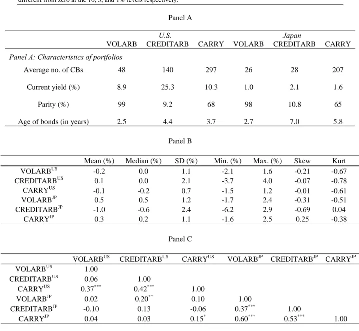
Table II reports the descriptive statistics of the three CA-related ABS factors. Panel A shows that on average the VOLARB factor has 48 (26) US (Japanese) CBs with an average current yield of 8.9% (1.0%) at an average parity of 99% (98%). This is consistent with VOLARB being, by design, a high gamma portfolio comprising of mostly at-the-money CBs.
The CREDITARB factor has on average, about three times as many US CBs (140 versus 48). The average current yield of 25.3% is substantially higher than that of VOLARB (8.9%)—a spread of 16.4%. Consistent with the design of the strategy, the
average parity of CBs in the CREDITARB factor is 9.2%. The spread of 16.4% in current yield is indicative of the increase in credit exposure between the two portfolios. Interestingly, for Japanese CBs, although the average parity drops from 98% for the VOLARB portfolio to 10.8% for the CREDITARB portfolio, neither the average current yield nor the average number of bonds in the two portfolios exhibit material change. This is symptomatic of the Japanese market where investors are simply not sufficiently rewarded for taking credit risk given the low level of interest rate—the current yield of the CREDITARB factor did increase by over 100% compared to the VOLARB factor (2.1% versus 1.0%), but in absolute terms, it is merely an increase of 1.1% for placing capital at default risk.
Consistent with the less restrictive selection criteria, the average number of CBs in the CARRY factor for the US (Japanese) is the highest among the three CA-related ABS factors—at 297 (207). The average parity of the CBs for the CARRY factor is 68% (65%) for the US (Japanese) CBs. The average current yield of CBs in the US (Japanese) CARRY factor is 10.3% (1.6%).
Finally, it is interesting to note the average age of the CBs in the three CA-related ABS factors. The bonds selected for the US VOLARB factor are the youngest (average age of 2.5 years). This is consistent with the fact that CBs tend to be issued almost at-the-money. Older, and therefore shorter maturity CBs, tend to be included in the CREDITARB factor—the same pattern appears to be the case for both the US and Japanese CBs.
All three CA-related ABS factors have daily returns spanning the sample period from January 1993 to August 2002. Panels A and B of Figure 1 plot the cumulative returns of the US and Japanese CA-related ABS factors over our sample period. Several features are worthy of note. During the post-LTCM period, CREDITARB were profitable factors in the US as were VOLARB and CARRY in Japan. This suggests that a globally diversified approach to executing CA strategies works better than a narrowly focused application of a single strategy in a specific country.
Since CA hedge fund returns are only available on a monthly basis, we compound the daily CA-related ABS factor returns into monthly returns. Table II Panel B provides the descriptive statistics of these monthly returns over our sample period.
Among the US factors, CREDITARB has the highest average return of 0.1% per month—consistent with the sizeable average current yield of the CREDITARB factor reflecting a high credit risk premium among US CBs used in this strategy. Among the Japanese factors, the VOLARB factor has the highest average return of 0.5% per month. In contrast, Japanese CREDITARB factor has a negative average return of -1.0% per month over our sample period—consistent with our earlier observation that investors were poorly rewarded for bearing the credit risk inherent in Japanese CBs.
Finally, Table II Panel C provides the correlations between the US and Japanese ABS factors. The US CARRY factor has returns that are correlated with the returns of the other two US CA-related ABS factors. However, the US VOLARB factor returns and CREDITARB factor returns have a low correlation. For Japanese CBs, the three CA-related ABS factors’ returns are significantly corCA-related with each other, whereas the US and Japanese CA-related ABS factors are generally uncorrelated. These low correlations
suggest that a convertible arbitrageur can attain significant diversification benefits by implementing these different trading strategies across the two markets.
III. Empirical Methodology and Results
III.A. Components of CA Hedge Fund Returns
It is reasonable to broadly divide CB investors into two groups—long-term holders of CBs and short-term traders in the CB market. We use CB mutual funds to
proxy the long-term holders of CBs, and CA hedge funds to proxy short-term traders acting like market-makers in the CB market.
Conceivably, in the process of market making, CA hedge funds hold net-long inventory of CBs. Although this net-long inventory position may vary over time, in an illiquid CB market, it is unlikely that a net-short inventory position can persist. We can therefore think of a CA hedge fund’s return comprising of two parts—a passive component and an actively managed component. One can capture the return to the
passive component by regressing the CA hedge fund returns on CB mutual fund returns. The return characteristic of the active component of a CA hedge fund return can then be captured by the CA-related ABS factor returns.
We use the Vanguard Convertible Securities mutual fund (VG), one of the largest mutual funds investing in CBs, as our proxy for CB mutual funds. Implicit in the Vanguard fund returns are the costs associated with acquiring and carrying a long position in the CB market and therefore better reflect the investing experience of long-term holders of CBs.19
19
As opposed to the returns of a CB index which typically does not adjust for transactions costs and may not be investable in its entirety.
Specifically, we model the passive component of CA hedge fund returns using the following regression:
CAt =λ0+λ1VGt+πt (9)
where, CAt is the month t excess-return (in excess of risk-free rate) on CA indexes, VGt is the month t excess return on the Vanguard Convertible Securities mutual fund, and
t
π is the residual left unexplained by the passive component.
III.B. Representative portfolios of the CA Hedge Fund Universe
As there is no universally accepted proxy for the market portfolio of CA hedge funds, to ensure a broad representation of the CA hedge fund universe, we include three widely used CA indexes—the Centre for International Securities and Derivative Markets (CISDM), CSFB Tremont (CT), and Hedge Fund Research (HFR) CA indexes—in our analysis.20
Since hedge fund indexes are generally not investable, we also conduct our analysis using individual hedge fund data from the CISDM, CT, and HFR databases. Agarwal, Daniel, and Naik (2005) report little overlap between these databases. Further, the individual funds in these databases may differ from those included in the indexes.21
Hence, we identify 155 unique CA funds from the three databases during our sample period (Jan 1993 to Aug 2002). Figure 2 is a Venn diagram showing the distribution of these funds across these databases. It shows that the databases overlap but do not provide
20
This allows us to test the robustness of our results to the differences in the constituents of these indexes and their construction methodology. For example, HFR weights all funds equally while CT gives higher weight to larger funds.
21
For example, CT indexes require funds to have a minimum AUM of $50 million and a minimum track record of one year.
identical coverage. A majority of funds come exclusively from CT (about 48% or 74 funds) and HFR (about 22% or 34 funds) databases.
To complement the CA indexes provided by data vendors, we construct an equally-weighted portfolio (EW) of these 155 CA funds. Our model of CA hedge fund returns assumes an illiquid CB market with unequal access to financing and differential transactions costs among economic agents. It follows that economies of scale may exist favoring larger CA hedge funds. For example, larger funds may enjoy these economies of scale in engaging arbitrage-like activities compared to the smaller CA hedge funds. To investigate this possibility, we also construct two equally-weighted sub-portfolios of CA funds –SMALL and BIG. Here SMALL (BIG) portfolio consists of funds with below-median (above-below-median) AUMs as of the end of previous month. These two sub-portfolios are rebalanced monthly.
In total, we examine three CA indexes and three CA portfolios representing different aspects of the CA hedge fund universe—CISDM, CT, HFR, EW, SMALL and
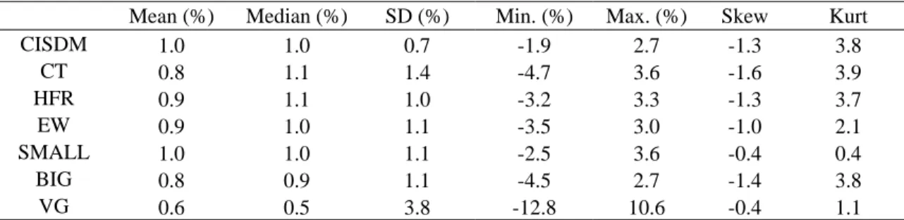
BIG. Table III reports the descriptive statistics of monthly returns of CA indexes, CA portfolios, and VG. Panel A shows the mean (median) return for the indexes and portfolios ranges from 0.8% to 1.0% (0.9% to 1.1%) while the standard deviations (SDs) ranges from 0.7% to 1.4% over our sample period. The return on VG is slightly smaller with mean (median) return of 0.6% (0.5%) while the SD is much higher at 3.8%.
Panel B reports the correlations among the different CA indexes, CA portfolios, and VG. As expected, we find that the CA indexes and portfolios are highly correlated with each other (correlations ranging from 0.70 to 0.95). Their correlation with VG is positive but lower in magnitude ranging from 0.35 to 0.61. Finally, Table III Panel C
provides the correlations among the CA indexes, CA portfolios, VG, and our CA-related ABS factors. In general, the CA indexes and CA portfolios show a positive correlation with all three CA-related ABS factors in the US and Japan (with the sole exception of Japanese CREDITARB factor) suggesting that these ABS factors are the important drivers of CA returns.
III.C. Multivariate Analysis of CA Hedge Fund Returns
Table IV Panel A reports the results in estimating the passive component of our three CA indexes and three individual hedge fund portfolios based on equation (9). The coefficient on VG is positive and significant for all the indexes and portfolios of CA hedge funds with magnitudes ranging from 0.10 to 0.18. This is consistent with our conjecture that there is a passive component to CA hedge fund returns. The magnitudes of the slope coefficients, on the other hand, suggest that there is only limited exposure of CA hedge fund returns to a passive, long-only strategy. The intercept,λ0, in each and every case is positive and significant suggesting that CA hedge funds engage in active strategies that adds value over and above a passive long-only position in CBs.
The results in Table IV Panel A suggest that the passive holding of inventory in CBs does not entirely explain the risks and rewards of CA strategy. Clearly, CA funds
actively manage the risk of their inventory by hedging the different risks associated with CBs such as equity risk, credit risk, and interest rate risk. Therefore, our CA-related ABS factors should be able to better explain the risk-return characteristics of CA hedge funds. We expand equation (9) by including the CA-related ABS and FXRET factors as
0 1 2 3
4 5 6 7
US US US
t t t t t
JP JP JP
t t t t t
CA VG VOLARB CREDITARB CARRY
VOLARB CREDITARB CARRY FXRET
θ ϑ θ θ θ
θ θ θ θ ψ
= + + + +
+ + + + + (10)
Table IV Panel B summarizes the results from the above regression. The results confirm that in addition to the exposure to the passive strategy proxied by VG, CA hedge funds have significant exposures to a number of CA-related ABS factors. In particular, CA hedge funds show significant loadings on the CARRY factors in US and Japan.
We also observe varying exposures to the CA-related ABS factors for the different CA indexes and portfolios suggesting a fair amount of heterogeneity across them. Finally, there is a considerable improvement in adjusted-R2. . This is particularly
true for CT index, the EW and BIG portfolios. Notice that the intercepts for CT index and BIG portfolio are no longer statistically significant. These results underscore the importance of including the CA-related ABS factors in modeling the returns of CA hedge funds.22
III.D. The Impact of Market Events and Sample Breaks
Although the VG returns reflect changes in the universe of CBs over time, it does so following a buy-and-hold strategy where CB inventory is held irrespective of market conditions. Unlike market makers in publicly traded securities, CA hedge funds are not mandated to absorb inventory at a given price. Therefore, their exposure to adverse selection risk is likely to be less than that of conventional market-makers. However, during events of extreme illiquidity, they too will exhibit return characteristics similar to
22
One may argue that the hedge fund returns are net-of-fees while those on our ABS factors are not. Therefore, for robustness, we also conduct our analysis with gross of fees returns, computed (following Agarwal, Daniel, and Naik, 2005 methodology) on portfolios constructed from CA hedge funds, and find similar results (not reported for brevity).
those resulting from adverse selection risk. The LTCM episode in 1998 enables us to shed light on the impact of a systemic liquidity squeeze on CA hedge funds and how they respond to extreme market events.
To model this, we follow recent work by Fung and Hsieh (2004a) and Fung, Hsieh, Naik and Ramadorai (2005). In these two studies, the authors provide strong evidence of structural breaks in hedge fund returns due to major market events like the LTCM crisis and the ending of the Internet Bubble. However, market events may affect different hedge fund strategies differently. We investigate this issue for the CA hedge funds by estimating the following structural break model accounting for LTCM crisis:
1 2 3 4
5 6 7 8
US US US
t t t t t
JP JP JP
t t t t t
CA VG VOLARB CREDITARB CARRY
VOLARB CREDITARB CARRY FXRET
ξ ω ω ω ω
ω ω ω ω κ
= + + + +
+ + + + + (11)
where, ξ is the intercept and ωi are slope coefficients defined as ξ ξ ξ= 0+ 1D and
0 1 , 1, 2,...,8
i i i D i
ω ω= +ω = , and pre-LTCM period (or structural break) dummy, D,
takes the value of 1 before LTCM crisis (before Oct 1998) and equals 0 otherwise. The other variables are as in equation (10). ωi0denotes the average factor loading during our sample period while ωi1denotes the incremental factor loading during the pre-LTCM period.
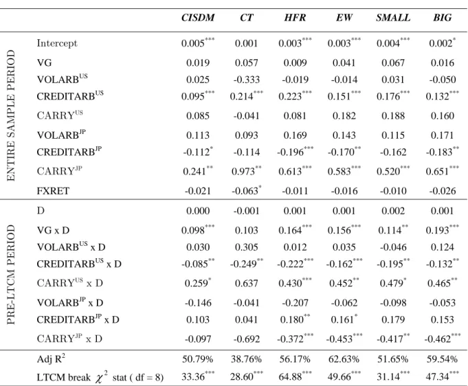
Table V reports the results. To test the hypothesis of a structural break due to the LTCM crisis, we perform the F-test forξ ω1= 11 =ω21=…=ω81 =0 using White’s (1980) heteroskedasticity-consistent covariance matrix estimator. We find significant Chi-square test statistics in all six cases along with a number of significant interaction terms suggesting the presence of a structural break corresponding to the LTCM crisis.
Fung and Hsieh (2004a) and Fung, Hsieh, Naik and Ramadorai (2005) reported another structural break around the end to the Internet bubble circa March 2000 for diversified portfolios of hedge funds. To check this possibility, we include another dummy in equation (11) for the post-March 2000 period. In results (not reported), we find this dummy to be mostly insignificant while the dummy for the LTCM event continues to be highly significant. This is consistent with the notion that unlike the LTCM event that affected both fixed-income and equity markets, the Internet bubble break was primarily an equity market event, and therefore had little impact on the CB market.
Table V provides the average factor loadings over the entire sample period (top half of the table) and the incremental loadings during the pre-LTCM period (bottom half of the table). Although the CA indexes and portfolios do not show significant exposure to VG over the entire sample period, they exhibit significantly positive exposure to passive long-only position in CBs (coefficient for VGxD term) during the pre-LTCM period. This is corroborated in Figure 3 where we plot the cumulative returns of VG and the three CA indexes. The performance of CA indexes is practically indistinguishable from that of VG during the pre-LTCM period. In contrast, CA indexes continue to perform well while VG’s performance deteriorated subsequently.
Another striking result from Table V is the significant change in the exposure to the US CREDITARB factor. Although over the entire sample period, the CA indexes and portfolios have a long exposure to this factor, prior to the LTCM event, it was significantly lower as suggested by the negative and significant slope coefficients on the interaction term (CREDITARBUS x D). Thus, after the adjustment for sample break, there is now a clear pattern of exposure in favor of the US CREDITARB factor. This is
consistent with the expansion of credit spread due to the LTCM event where a higher risk premium is offered to providers of liquidity and the CA hedge funds took advantage of that.
In contrast to our earlier results that did not allow for structural break (Table IV), the US CARRY factor now shows significant positive loading only during the pre-LTCM event. Also earlier results in Table IV reveal that convertible arbitrageurs had significant exposure to the CARRY factor in Japan. This pattern of exposure is largely unaffected by the sample break analysis as confirmed by the results in Table V.23
Overall, these results suggest that convertible arbitrageurs respond to extreme market events by changing their choice of trading strategies whilst providing liquidity to the CB market. The intercepts for five out of the six CA portfolios remain statistically significant and positive after adjusting for sample break. The magnitude of these
abnormal returns range from 20 basis points a month (BIG) to 50 basis points a month (CISDM), net of all fees and expenses. These are sizeable abnormal returns and did not escape the attention of hedge fund investors. Capital flow into CA hedge funds grew steadily throughout our sample—from under $5 billion during early 1993 to well over $65 billion of asset under management (“AUM” for short) by August 2002. In particular, the AUM growth accelerated towards the last quarter of 1999 and nearly trebled by August 2002. However, as we noted in earlier discussions, the number of Japanese CB issues halved over the same period—see Panel C of Table I. This begs the question as to
23
Looking at Figure 1 Panel B, one would have expected that VOLARB factor in Japan would be a significant driver of CA hedge fund returns. However, the results in Table V do not support this conjecture. This may be due to high correlation between Japanese CARRY and VOLARB factors (0.6; see Table II Panel C).
how CA hedge funds responded to these substantial changes to their environment. In the next section, we extend our model to glean insight into this question.
III.E. How does the supply and demand of CBs affect convertible arbitrageurs?
CA hedge funds play an important role of supplying liquidity to the CB market. As such, their performance must be sensitive to the imbalances between supply of and demand for CBs over time. To estimate the total supply of CBs, we aggregate the market capitalization of all outstanding CBs every month.24 Part of this supply flows into the
portfolio of long-terms investors, such as CB mutual funds. There is another group of active, but short-term investors of CBs with a long-only bias—these are CB hedge funds classified by HFR as fixed income convertible bond (“FICB” for short) hedge funds.25
Unlike CA hedge funds, these FICB hedge funds do not engage in arbitrage-like strategies, rather, they tend to rely on security selection and market timing strategies to achieve performance. Consequently, we include their demand for CBs together with the CB mutual funds in order to deduce the floating supply of CBs to which CA hedge funds are providing liquidity. We refer to this floating supply of CBs as the net supply of CBs by subtracting the AUM of all CB mutual funds and FICB hedge funds from the total market capitalization of all outstanding CBs each month.26
Next we turn to the question of estimating the demand for CBs from the providers of short-term liquidity.27 We approximate the demand for CBs by aggregating the total
24
The market cap of Japanese CBs are converted into US dollars using the monthly Yen/USD exchange rate before adding it to the market cap of US CBs.
25
Hedge Fund Research (HFR) defines the FICB strategy as “…primarily long only convertible bonds”. Source: http://www.hedgefundresearch.com/index.php?fuse=indexes-str#2282
26
The AUM data for the CB mutual funds is from the CRSP mutual fund data base (funds with Strategic Insight (SI) objective as “CVR”) and the FICB hedge fund data is from the HFR database.
27
AUM of all the 155 CA hedge funds at the end of each month in our sample. Figure 4 depicts the time-series variation in the net supply of and demand for CBs during our sample period (Jan 1993 to Aug 2002). It is interesting to observe the co-movement of demand and supply over time. Although it appears that the supply of CBs appears to far exceed our estimate of demand, it is important to note that CA hedge funds are leveraged
holders of CBs. Therefore, their AUM actually reflects a lower bound of the demand of CA hedge funds.
To capture the imbalances between supply and demand, we use the ratio of supply to demand (“SUPDEM” for short) each month. Another way to think about the SUPDEM is that it represents the investment opportunities available in the CB market. Merton’s (1973a) intertemporal CAPM suggests that the risk factors in APT-type multifactor model should reflect the future stochastic investment opportunity set. We introduce
SUPDEM as an additional variable in equation (11) and estimate the following regression:
1 2 3 4
5 6 7 8
9 1
US US US
t t t t t
JP JP JP
t t t t
t t
CA VG VOLARB CREDITARB CARRY
VOLARB CREDITARB CARRY FXRET
SUPDEM
α β β β β
β β β β
β − χ
= + + + +
+ + + +
+
(12)
where,α α α= 0+ 1D, βi =βi0+βi1D, i=1, 2,..., 9and SUPDEMt-1 is lagged value of supply to demand ratio.28 The other variables are as in equation (11). We report the
results for the three CA indexes and three CA portfolios in Table VI.
There are two striking results from the extended model in equation (12). First, with the exception of the CT index, practically all factor loadings that were statistically significant (insignificant) prior to the introduction of the supply-demand factor (see Table
28
Since the investment opportunities need to be in the information set of CA hedge fund manager, we take the SUPDEM as of the end of previous month. For robustness, we repeat our analysis using contemporaneous SUPDEM and find qualitatively similar results.
V) remain statistically significant (insignificant). Furthermore, the magnitudes of the factor loadings remain largely unchanged with the addition of the supply-demand factor in the model. Overall, our earlier conclusion regarding the existence of a sample break continues to hold with the introduction of this new supply-demand factor.
Second, the key impact of introducing the new supply-demand variable is to drive the abnormal returns of the CA portfolios (the intercept terms of the regression results reported in Table V) downwards—from being positive and statistically significant for five out of six of the CA sub-portfolios to insignificantly different from zero in all cases except CT, where it is significant but negative. This shows that after accounting for the investment opportunities for the CA strategy, in general, CA hedge funds no longer
deliver abnormal returns. One interpretation of this result is that non-factor related returns are simply a liquidity premium offered by the CB market.
Interestingly, for the overall sample period, we find that the supply-demand factor (SUPDEMt-1) is positive and significant for the CT index and all the three portfolios (EW, SMALL, and BIG). This is consistent with the notion that the larger the supply of CBs relative to the demand of CBs, the better the investment opportunities for convertible arbitrageurs. We find that a one-sigma change in SUPDEMt−1has a positive impact on the returns of all the indexes, the EW and Big portfolios both before and after the structural break. In particular, we find that a one-sigma change in SUPDEMt-1 increases the monthly returns on CISDM index before (after) the break by 0.01% (0.09%), on CT index by 0.13% (1.43%), and on HFR index by 0.05% (0.05%). It also increases the monthly returns on our EW and BIG portfolios before (after) the break, namely EW portfolio by 0.04% (0.32%), and BIG portfolio by 0.10% (0.38%).
In contrast, a one-sigma change in SUPDEMt-1 actually impairs the performance of the SMALL portfolio by 0.03% before the break, but enhances returns by 0.30% after the break. These figures are economically significant relative to the mean (median) returns of CA indexes and portfolios ranging from 0.8% to 1.0% (0.9% to 1.1%) (see Table III Panel A). This underscores the importance of demand-supply factor in determining the returns on CA strategy.
As discussed in the introduction, we believe that the unprecedented losses CA hedge funds experienced in early 2005 were driven by changes in the supply-demand factor. On the demand side, the AUMs of CA hedge funds kept rising from mid-2003 till end of 2004, while on the supply side, the new issuance of CBs kept dwindling over that period. This resultedin an enormous supply-demand imbalance, which led to a six-standard-deviation drawdown in the performance of CA funds in the first-half of 2005.29
This “out-of-sample,” unprecedented event confirms the importance role of our supply-demand factor in models CA strategies.
Taken together, these results provide strong evidence on this set of strategy-specific factors—CA-related ABS factors and supply-demand factor—being important determinants of the risks and rewards of CA strategy. These strategy-specific factors together with the inclusion of a structural break arising from extreme market events such as the LTCM crisis substantially improved the explanatory power of the one-factor VG model. Table VI shows that adjusted R2 ranges from 45% to 62%, which is a substantial
improvement from the adjusted R2 achieved by the one-factor VG model (Table IV Panel
A, 11% to 36%).
29
Interestingly, the performance of long-only CB funds (VG) suffered a loss of only 0.9 standard deviations. This shows that convertible arbitrageurs by virtue of their providing liquidity in the CB market are more sensitive to demand-supply conditions.
Finally, the SMALL portfolio which started with a higher adjusted R2 in the
one-factor (VG) model (36.26% in Table IV Panel A) to that of the BIG portfolio (26.77% in Table IV Panel A) ended with a lower adjusted R2 than the BIG portfolio after the
arbitrage-like ABS factors are included (see Tables V and VI). This suggests that larger funds may be engaging in more arbitrage-like activities compared to smaller funds.
IV. Concluding Remarks
Majority of convertible bonds transact in opaque over-the-counter markets. Consequently, there is no direct way of observing the trading strategies employed by financial intermediaries such as market-makers in these markets. The last decade has witnessed a continuous migration of this intermediary function from the investment banks to hedge funds. More specifically into the hands of what has come to be known as convertible arbitrage hedge funds. Our analysis of these specialized hedge funds provides a rare glimpse into the strategies engaged by arbitrageurs who provide liquidity to the convertible bond market. We do so by directly modeling the trading strategies that a convertible arbitrageur could use to manage an inventory of convertible bonds. Our approach lends interesting insights into the nature of financial intermediation in hard to observe Over-The-Counter (OTC) markets.
Using daily data from the underlying convertible bond and stock markets in the US and Japan, we construct three asset-based style factors for the convertible bond market – volatility arbitrage, credit arbitrage, and positive carry. Our empirical results show that these factors explain a large proportion of the return variation in convertible arbitrage hedge funds. In addition, we show that convertible arbitrageurs escaped some
of the losses experienced by long-only convertible bond mutual funds by changing their risk exposures in response to the LTCM crisis. Finally, our results reveal the important role played by supply-demand imbalances in determining the profitability of convertible arbitrage strategy. This in turn implies that unsystematic return to convertible arbitrageurs is analogous to a premium earned for providing liquidity to the convertible bond market.
References
Agarwal, Vikas, and Narayan Y. Naik, 2004, “Risks and Portfolio Decisions involving Hedge Funds,” Review of Financial Studies 17(1), 63-98.
Agarwal, Vikas, Daniel, Naveen D., and Narayan Y. Naik, 2005, “Role of managerial incentives, flexibility, and ability: Evidence from performance and money flows in hedge funds,” Working Paper, Georgia State University and London Business School.
Alexander, Gordon J, and Roger D Stover, 1977, “Pricing in the new issue convertible debt market,” Financial Management 6, 35-40.
Almazan, Andres, Keith C. Brown, Murray Carlson, and David A. Chapman, 2004, “Why constrain your mutual fund manager?,” Journal of Financial Economics 73, 289-321. Altman, Edward I., 1989, “The Convertible Debt Market: Are Returns Worth the Risk?,”
Financial Analysts Journal, 45.
Ammann, M., Kind, A. and Wilde C., 2004, “Are convertible bonds underpriced? An analysis of the French market,” Journal of Banking & Finance, 27, 635-653.
Bhattacharya, Mihir, 2000, Convertible securities and their valuation, in Frank J. Fabozzi, ed.:
The Handbook of Fixed Income Securities (Mc-Graw Hill, New York).
Brennan, Michael J., and A. Kraus, 1987, “Efficient financing under asymmetric information,” Journal of Finance 42, 1225-1243.
Brennan, Michael J., and Eduardo S. Schwartz, 1977, “Convertible Bonds: Valuation and Optimal Strategies for Call and Conversion,” Journal of Finance 32, 1699-1715.
Brennan, Michael J., and Eduardo S. Schwartz, 1980, “Analyzing Convertible Bonds,”
Journal of Financial and Quantitative Analysis 15, 907-929.
Brennan, Michael J., and Eduardo S. Schwartz, 1988, “The case for convertibles,” Journal of
Applied Corporate Finance 1, 55-64.
Brown, William Anthony, 2000, “Convertible Arbitrage: Opportunity & Risk,” Tremont
White Paper, November 2000.
Calamos, Nick, 2003. Convertible arbitrage: insights and techniques for successful hedging (John Wiley, Hoboken, N.J.).
Carayannopoulos , P., 1996. “Valuing convertible bonds under the assumption of stochastic interest rates: An empirical investigation”. Quarterly Journal of Business and Economics 35 (3), 17–31.
Carayannopoulos, Peter, and Madhu Kalimipalli, 2003, “Convertible Bond Prices and Inherent Biases,” forthcoming Journal of Fixed Income.
Chan, Alex W.H., and Nai-fu Chen, 2004, “Convertible Bond Pricing: Renegotiable Covenants, Seasoning and Convergence,” Working Paper, University of Hong Kong and University of California, Irvine.
Constantinides, G.M., and B.D. Grundy, 1989, “Optimal investment with stock repurchase and financing as signals,” Review of Financial Studies 2, 445-465.
Dialynas, Chris P., Sandra Durn, and John C. Jr. Ritchie, 2000, “Convertible securities and their investment characteristics,” in Frank J. Fabozzi, ed.: The Handbook of Fixed Income
Securities (Mc-Graw Hill, New York).
Das, S. R. and R. K. Sundaram, 2004, “A Simple Model for Pricing Securities with Equity, Interest rate and default risk,” Working paper, New York University and University of California, Santa Clara.
Davis, M. and F. R. Lischka, 1999, “Convertible bonds with market risk and credit risk,” Working paper, Tokyo-Mitsubishi International PLC.
Deli, D.N., and R. Varma, 2002, “Contracting in the investment management industry: evidence from mutual funds,” Journal of Financial Economics 63, 79-98.