Vol. 00, No. 0, Xxxxx 0000, pp. 000–000
issn0030-364X|eissn1526-5463|00|0000|0001 doi10.1287/xxxx.0000.0000°c0000 INFORMS
Approximation Algorithms for Capacitated
Stochastic Inventory Control Models
Retsef Levi
Sloan School of Management, MIT, Cambridge, MA, 02139., [email protected],
Robin O. Roundy
School of ORIE, Cornell University, Ithaca, NY 14853, [email protected],
David B. Shmoys
School of ORIE and Dept. of Computer Science, Cornell University, Ithaca, NY 14853., [email protected],
Van Anh Truong
School of ORIE, Cornell University, Ithaca, NY 14853, [email protected],
We develop the first algorithmic approach to compute provably good ordering policies for a multi-period, capacitated, stochastic inventory system facing stochastic non-stationary and correlated demands that evolve over time. Our approach is computationally efficient and guaranteed to produce a policy with total expected cost no more than twice that of an optimal policy. As part of our computational approach, we propose a novel scheme to account for backlogging costs in a capacitated, multi-period environment. Our cost-accounting scheme, called the forced marginal backlogging cost-accounting scheme, is significantly different from the period-by-period accounting approach to backlogging costs used in dynamic programming; it captures the long-term impact of a decision on system performance in the presence of capacity constrains. In the likely event that the per-unit order costs are large compared to the holding and backlogging costs, a transformation of cost parameters yields a significantly improved guarantee. We also introduce new semi-myopic policies based on our new cost-accounting scheme to derive bounds on the optimal base-stock levels. We show that these bounds can be used to effectively improve any policy. Finally, empirical evidence is presented that indicates that the typical performance of this approach is significantly stronger than these worst-case guarantees.
Subject classifications: Stochastic Inventory Control; Heuristics; Approximation Algorithms.
Area of review: Supply Chain Management.
History: Submitted August 2005. Revised July 2006, December 2006, May 2007, September 2007, September 2007.
1. Introduction
The periodic-review, capacitated inventory control problem for systems facing stochastic, non-stationary (time-dependent) demands that are correlated and evolve over time is an important classical problem that is widely recognized to be computationally challenging. We develop a new algorithmic approach to compute the order quantity for such a system. We build on the work of Levi et al. (2007), who used a marginal holding cost accounting scheme and cost balancing techniques to derive the first policies with worst-case performance guarantees for uncapacitated models. In this paper, we introduce a novel marginal backlogging cost accounting scheme that, in combination with their techniques, lead to analogous results for the much harder capacitated model. We believe that our new cost accounting scheme will have applications in many other settings. Our algorithm is guaranteed to compute a solution of total expected cost no more than twice that of an optimal policy for any instance of the problem. The algorithm is computationally efficient and implementable without having to enumerate exhaustively future scenarios and corresponding future decisions. In particular, the decision made in the current period is unaffected by any future decision. Thus, it can be implemented efficiently even in the presence of complex demand structures.
Specifically, we consider single-item models with one location and a finite planning horizon of T discrete time periods. The demands over the T periods are random variables that can be non-stationary and correlated. The costs consist of a per-unit, time-dependent ordering cost, a per-unit holding cost for carrying excess inventory from period to period and a per-unit backlogging cost, which is a penalty incurred, in each period, for each unit of unsatisfied demand (where all shortages are fully backlogged). There is a time-dependent capacity constraint on the number of units ordered in each period and a lead time between the time that an order is placed and the time that it actually arrives. The capacity constrains and lead times may be stochastic.
Capacitated problems are inherently more difficult computationally compared to their uncapac-itated counterparts. The constraint on capacity makes future costs heavily dependent on current decisions. Myopic policies, which do not consider the impact of a decision made in the current period on the costs incurred in future periods, seem to perform well for some scenarios in uncapac-itated systems and are even optimal in some settings (seeVeinott (1965), Ignall and Veinott (1969) Iida and Zipkin (2001), and Lu et al. (2006)). However, when applied to capacitated problems, they usually perform very poorly because they do not consider possible capacity limitations in future periods.
In this work, we introduce a look-ahead backlogging cost-accounting scheme, called the forced marginal backlogging cost-accounting scheme, to capture the long-term impact of current decisions on future costs in the presence of capacity constrains. Our new cost accounting scheme assigns to the decision in each period all of the expected backorder costs that, once this decision is made, become inevitable; that is, they are unaffected by any decision made in future periods, and are dependent only on future demands. The forced marginal backlogging cost reduces to the traditional backlogging cost when the capacity is infinite; thus, it is a generalization of the traditional back-logging cost. Finally, as discussed in Section 3.1, it is straightforward to compute in most common scenarios.
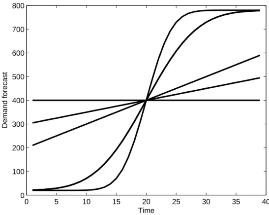
The key feature distinguishing the algorithms presented in this paper from those previously studied for capacitated systems is the treatment of correlation in demand across time as well as non-stationarity. Moreover, we allow observations of the past to change demand forecasts for the future. Our model also captures other important characteristics of a non-stationary environment: the parameters are fully time-dependent, including cost parameters and system capacity. An important application of demand correlation and non-stationarity is in the use of dynamic demand forecasts. These forecasts and the way they evolve over time provide vital information that can be used to find effective inventory control policies in dynamic and highly volatile demand environments. The assumptions that we make on the demand distributions in this work are mild enough to generalize all of the currently known approaches in the literature to model correlation and non-stationarity of demand over time. These include classical approaches like themartingale model of forecast evolution model(MMFE), exogenous Markovian demand, time series, order-one auto-regressive demand and random walks. For an overview of the different approaches and models, and for relevant references, we refer the reader to Iida and Zipkin (2001) and Dong and Lee (2003).
High correlation between demands across different periods in non-stationary and dynamic envi-ronments presents a considerable challenge to computing, or even approximating, optimal inventory control policies. The dominant paradigm in almost all of the existing literature has been to for-mulate multi-period capacitated models using dynamic programming. The optimization problem is defined recursively over time using subproblems for each possible state of the system. The state usually consists of a given time period, the level of inventory at the beginning of the period, the resulting conditional distribution of future demands over the rest of the horizon, and possibly more information that is available by that period. For each subproblem, an optimal solution is computed to minimize the expected overall discounted cost from the current point to the end of the horizon. This framework has turned out to be very effective in characterizing the structure of the optimal
policy of the overall system. Assuming stationary linear costs and independent and identically distributed (i.i.d.) demands, Federgruen and Zipkin (1986a,b) showed that a modified, base-stock policy is optimal under infinite-horizon average-cost and discounted cost criteria. They established the existence of a target inventory level such that the optimal policy aims to keep inventory levels as close as possible to that target. When the inventory level at the beginning of the period is above the target level, the optimal policy does not order. When the inventory level at the beginning of the period is below the target level, it might not be possible to order up to the target level because of the capacity constraint. In this case, the order placed would be up to capacity. Tayur Kapuscinski and Tayur (1998) and Aviv and Federgruen (1997) derived the optimal policy in the same settings, but for independent cyclical demands.
Axs¨ater (1990) is the first to introduce the notion of matching between pairs of demand and supply units. Specifically, he observes that in a distribution system with a single depot and multi-ple retailers, a supply unit ordered by a retailer can be used to fill a corresponding demand unit following a certain order. He matches this pair of units and evaluates the corresponding expected holding cost. Katircioglu and Atkins (1996) have used this observation to analyze the optimal poli-cies in unit demand inventory systems. For the uncapacitated periodic-review stochastic inventory control problem, Muharremoglu and Tsitsiklis (2001) have proposed an alternative approach to the dynamic programming framework. They have observed that this problem can be decoupled into a series of unit supply-demand subproblems, where each subproblem corresponds to a single unit of supply and a single unit of demand that are matched. This novel approach enabled them to substantially simplify some of the dynamic programming based proofs on the structure of opti-mal policies, as well as to prove several important new structural results. In particular, they have established the optimality of state-dependent base-stock policies for the uncapacitated model with general Markov-modulated demand. Using this unit decomposition, they have also suggested new methods to compute the optimal policies. However, their computational methods are essentially dynamic programming approaches applied to the unit subproblems, hence they suffer from similar problems in the presence of correlated and non-stationary demand. Although our approach is very different from theirs, we use some of their ideas as technical tools in some of the proofs. Janaki-raman and Muckstadt (2003) have extended this approach to capacitated models and established the optimality of state-dependent modified base-stock policies for models with Markov-modulated demand.
Unfortunately, the rather simple forms of these policies do not always lead to efficient algorithms for computing the optimal policies. Complex demand structures, such as the one we consider in this work, cause the state space of the corresponding dynamic programs to explode (see Iida and Zipkin (2001), and Dong and Lee (2003) for relevant discussions on the MMFE model). There does not exist at present, nor is there likely to be developed, an efficient algorithm to solve these dynamic programs to optimality, even for the uncapacitated model. The difficulty comes from the fact that we need to solve ‘too many’ subproblems, a phenomenon known as the curse of dimensionality. To date, computational procedures have been made tractable only under assumptions of simple demand structures. If the demands in different periods are independent, the corresponding dynamic programs are relatively straightforward to solve. Dynamic programming can still be tractable for uncapacitated models with Markov-modulated demand but under rather strong assumptions on the structure and the size of the state space of the underlying Markov process (see, for example, Song and Zipkin (1993) and Chen and Song (2001)). Tayur (1992) uses the shortfall distribution and the theory of storage processes to derive an efficient computational method for computing the optimal policy in the stationary cost, i.i.d. demand, average-cost case. Roundy and Muckstadt (2000) showed how to obtain approximate base stock levels, also for the stationary cost and i.i.d. demand case, by approximating the distribution of the shortfall process. Kapuscinski and Tayur (1998) proposed a simulation-based technique using infinitesimal perturbation analysis to compute the optimal policy for capacitated problems with independent, cyclical demands.
There have been heuristic approaches to compute order quantities for capacitated problems. However, we are aware of very few attempts to analyze the worst-case performance of heuristics and most bounds derived are dependent on the particular input (see, for example, Lu et al. (2006)). To the best of our knowledge, there are no other policies for stochastic inventory control models with constant worst-case performance guarantees. Metters (1997) found heuristics for capacitated, lost-sales problems with independent, cyclical demands. Chan (1999) have considered heuristics for uncapacitated and capacitated multi-item models. Instead of solving the one-period problem (as in the Myopic policy), they have added a penalty function to the one-period problem, which they called the Q-function. This function accounts for the holding cost incurred by the inventory left at the end of the period over the entire horizon. Their look-ahead approach with respect to the holding cost is somewhat related to our approach, though significantly different.
As we have already mentioned, this paper builds on the work of Levi et al. (2007). They give the first algorithms with a constant performance guarantee for the uncapacitated stochastic inventory control model with correlated, non-stationary demands; specifically, their algorithms always find solutions of total expected cost no more than twice the optimal. Their algorithms are based on two main ideas. First, they construct a look-ahead holding cost accounting scheme, called themarginal holding cost accounting scheme, to compute the additional holding costs incurred by units ordered in the current period throughout the entire horizon. Secondly, they usecost-balancingtechniques in that, in each period, they order exactly to balance the following two opposing costs: the conditional expected marginal holding cost against the conditional expected period backlogging cost a lead time ahead. Their approach relies heavily on the ability of the system to order in each period a ‘balancing quantity’ that equalizes the expected marginal holding cost and the expected backlogging cost in the period. In capacitated systems, the approach fails because this balancing quantity might not be attainable due to capacity constrains. Our forced marginal backlogging cost accounting scheme is designed to remedy this problem by reassigning backlogging costs more appropriately to the decisions that create them, enabling us to find a ‘balancing order quantity’ for capacitated systems. Suppose that in the current period the order placed was not up to capacity; we wish to account for the potential backlogging cost in future periods incurred directly by the decision not to use the full available capacity. Assume temporarily that we order up to capacity in each one of the periods. Suppose now that in the current period we do not order up to capacity. Then the expected marginal backlogging cost associated with the current period is the overall increase in the expected backlogging cost over the entire horizon resulting from this decision. In this way, our balancing policy for a capacitated system is able to achieve the same worst-case performance guarantee of 2, with surprisingly little additional computational effort. When applied to uncapacitated models the policies described in this paper are identical to the Dual-Balancing policies described by Levi et al. (2007). Thus, they can be viewed as generalizations of the original Dual-Balancing policies to capacitated inventory models.
We also use the marginal holding and forced marginal backlogging cost accounting schemes to derive additional semi-myopic policies, called the Lower-Myopic and Upper-Myopic policies. The policies provide lower and upper bounds on the optimal base-stock levels, respectively, which can be used in conjunction with any policy to achieve lower expected cost.
Furthermore, in Section 4.2 we show how to use standard cost transformations to improve the performance of the algorithms in many important settings (see also Levi et al. (2007)). These transformations yield a modified instance of the problem that is equivalent to the original one from an optimization perspective, but models only holding and backlogging costs. If the per-unit ordering cost is constant over time, then applying our algorithms to the modified instance yields an approximation algorithm with a worst-case guarantee of 2 with respect to the holding and backlogging costs, and which has the same total per-unit ordering cost as the optimal policy. More generally, when the ordering costs are large, the worst-case performance guarantee of the modified-cost Dual-Balancing policy will be much better than 2.
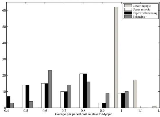
In Section 6 we test the typical performance of the balancing algorithms in two settings. We consider an inventory system that has i.i.d. demand (no correlations), and a demand distribution with an exponential tail, because the optimal policy can be computed analytically. (The motivation is to the test balancing policies at least in one environment, in which the optimal policy and cost are known.) However, balancing policies are most attractive in scenarios with complex demand structures, whereas optimal policies can not be computed and no provable good heuristics or reasonable lower bounds are known. Thus,we also consider the same set of test scenarios tested in Hurley et al. (2006), in which the uncapacitated versions of these algorithms were evaluated computationally. In these scenarios the demands and forecasts evolve according to the multiplicative MMFE model. Optimal policies are not computable and strong lower bounds do not exist, so we used the Myopic policy as a benchmark for evaluating performance. The performance of the Balancing policies is very robust. It was within 11% of optimal on average in the first test (always within 25%), and consistently improved upon myopic, by over 27%, on average and by over 50% in many scenarios.
The paper is organized as follows. In Section 2 we present the mathematical formulation of the periodic-review, capacitated, stochastic inventory control problem. In Section 3 we describe the forced marginal backlogging cost accounting scheme for the capacitated model. In Section 4 we describe the balancing policy and its worst-case analysis. We also extend the approximation results to the case of discrete demand and stochastic lead times (see Appendix C). In Section 5, we develop lower and upper bounds on the optimal inventory levels, and show how to use them to improve any policy. Section 6 contains our computational results. Appendix A contains a very simple, illustrative example for the case of integer-valued demand. In Appendix B we present a detailed description of the scenarios tested in the computational results.
2. Capacitated Periodic-Review Stochastic Inventory Control Problem
In this section, we provide the mathematical formulation of the capacitated periodic-review stochas-tic inventory problem and introduce some of the notation used throughout the paper. As a general convention, we distinguish between a random variable and its realization using capital letters and lower case letters, respectively. Script font is used to denote sets. We consider a finite planning horizon of T periods numbered t= 1, . . . , T (note that t and T are both deterministic unlike the convention above). The demands over these periods are random variables, denoted byD1, . . . , DT.
As part of the model, we assume that at the beginning of each period s, we are given what we call aninformation setthat is denoted byfs. The information setfscontains all of the information
that is available at the beginning of time periods. More specifically, the information setfsconsists
of the realized demands (d1, . . . , ds−1) over the interval [1, s), and possibly some more (external)
information denoted by (w1, . . . , ws). The information set fs in period sis one specific realization
in the set of all possible realizations of the random vectorFs= (D1, . . . , Ds−1, W1, . . . , Ws). This set
is denoted by Fs. In addition, we assume that in each period sthere is a known conditional joint
distribution of the future demands (Ds, . . . , DT), denoted by Is:=Is(fs), which is determined by fs (i.e., knowingfs, we also knowIs(fs)). For ease of notation, Dt will always denote the random
demand in periodt according to the conditional joint distribution Is for somes≤t, where it will
be clear from the context to which period s we refer. We will use tas the general index for time, andswill always refer to the current period. The only assumption on the demands is that for each s= 1, . . . , T, and each fs∈ Fs, the conditional expectation E[Dt|fs] is well defined and finite for
each periodt≥s. In particular, we allow non-stationarity and correlation between the demands of different periods.
In the periodic-review stochastic inventory control problem, our goal is to supply each unit of demand while attempting to avoid ordering it either too early or too late. In periodt, (t= 1, . . . , T) three types of costs are incurred, a per-unit ordering cost ct for ordering up to ut units, where
ut≥0 is the available order capacity in period t, a per-unit holding cost ht for holding excess
inventory from period t to t+ 1, and a per-unit backlogging penalty pt that is incurred for each
unsatisfied unit of demand at the end of period t. Unsatisfied units of demand are usually called
backorders. Backorders fully accumulate over time until they are satisfied. That is, each unit of unsatisfied demand will stay in the system and will incur a backlogging penalty in each period until it is satisfied. In addition, there is a lead time of L periods between the time an order is placed and the time at which it actually arrives. We first assume that the lead time is a known integerL. In Appendix C, we show that our policy can be modified to handle stochastic lead times under the assumption of no order crossing (i.e., any order arrives no later than those placed later in time). In Section 4.1, we show that extensions to the case of random capacities are straightforward.
There is also a discount factor α≤1. The cost incurred in period t is discounted by a factor of αt. Since the horizon is finite and the cost parameters are time-dependent, we can assume without
loss of generality that α= 1. We also assume that there is no speculative motivation for holding inventory or having back orders in the system. To enforce this, we assume that, for each t= 2, . . . , T−L, the inequalitiesct≤ct−1+ht+L−1andct≤ct+1+pt+Lare maintained (wherecT+1= 0). (If there is a discount factor, we require that αct≤ct−1+αLht+L−1 and ct≤αct+1+αLpt+L). We
also assume that the parameters ht, pt and ct are all non-negative. Note that the parameters hT
and pT can be defined to take care of excess inventory and back orders at the end of the planning
horizon. In particular,pT can be set sufficiently high so as to ensure that there are very few back
orders at the end of period T.
The goal is to find a feasible ordering policy (i.e., one that respects the capacity constraints) that minimizes the overall expected discounted ordering cost, holding cost and backlogging cost. We consider only policies that arenon-anticipatory, i.e., at times, the information that a feasible policy can use consists only offs and the current inventory level.
Throughout the paper we will use D[s,t] to denote the accumulated demand over the interval [s, t], i.e., D[s,t]:=
Pt
j=sDj. We will also use superscriptsP and OP T to refer to a given policyP
and the optimal policy respectively.
Given a feasible policy P, we describe the dynamics of the system using the following terminol-ogy. We let N It denote the net inventory at the end of periodt, which can be either positive (in
the presence of physical on-hand inventory) or negative (in the presence of back orders). Since we consider a lead time ofL periods, we also consider the orders that are on the way. The sum of the units included in these orders, added to the current net inventory is referred to as the inventory positionof the system. We let Xt be the inventory position at the beginning of periodtbefore the
order in period tis placed, i.e., Xt:=N It−1+
Pt−1
j=t−LQj (for t= 1, . . . , T), where Qj denotes the
number of units ordered in periodj (we will sometime denotePtj−=1t−LQj byQ[t−L,t−1]). Similarly,
we let Yt be the inventory position after the order in period t is placed, i.e., Yt=Xt+Qt. Note
that once we know the policy P and the information set fs∈ Fs, we can easily compute nis−1,xs
and ys, where again these are the realizations ofN Is−1, Xs and Ys, respectively.
3. Marginal Cost Accounting Scheme
In this section, we present a marginal cost accounting for stochastic inventory control problems with capacity constraints on the size of the order in each period. This extends and generalizes the marginal cost accounting discussed by Levi et al. (2007). Since this cost accounting approach is central for our approximation results, we explain it in detail, repeating some of the ideas of that paper. Our approach differs significantly from the traditional cost accounting approaches, which is based on standard dynamic programming.
We start by reviewing their cost accounting approach, which is called marginal cost accounting. The main idea underlying this approach is to account for all the expected costs associated with
the decision of how many units to order in periodt when this decision is made. More specifically, the decision in period t is associated with all the expected cost that, after that decision is made, become unaffected by any future decision, and are only dependent on future demands. In Levi et al. (2007) it was shown that in uncapacitated models, these costs are relatively easy to compute already in period t, even though they may include costs that are going to be incurred only in future periods. Taking this approach, Levi, P´al, Roundy and Shmoys have proposed a marginal holding cost accounting scheme. Their approach is based on the convention that units in inventory are consumed on a first-ordered-first-consumed basis. This implies that the overall holding cost of the qs units ordered in period s (i.e., the holding cost they incur over the entire horizon [s, T])
is a function only of future demands, and is independent of any future decision. Based on the assumption that inventory is consumed on a first-ordered-first-consumed basis, theqsunits on order
will be used to satisfy demand only when thexsunits presently in the system have been completely
consumed. Among these qs units, the number of those still remaining in inventory at the end of
periodj(where j≥s+L) is precisely (qs−(D[s,j]−xs)+)+. Each of these units incurs a cost ofhj.
More specifically, conditioning on an information setfs∈ Fs, the marginal holding cost is defined
to be (assuming again that α= 1) PTj=s+Lhj(qs−(D[s,j]−xs)+)+. Observe again that for each
non-anticipatory policy P, if conditioned on some ft∈ Ft, the inventory position at the beginning
of period t, denoted by xP
t, is known deterministically. In addition, once the order in period s is
determined, the backlogging cost a lead time ahead in periods+L, i.e.,ps+L(D[s,s+L]−(xs+qs))+,
is also dependent only on the future demands. This leads to a marginal cost accounting. For each feasible policyP, letHP
t be the ordering and holding cost incurred over the interval [t, T] by theQPt
units ordered in periodt(fort= 1, . . . , T), and let ΠP
t be the backlogging cost incurred a lead time
ahead in periodt+L(t= 1−L, . . . , T−L). That is,HP
t =ctQPt +
PT
j=t+Lhj(QPt −(D[t,j]−XtP)+)+
and ΠP
t :=pt+L(D[t,t+L]−(XtP+L+QPt))+ (where Dj:=dj with probability 1 and QPj =qj is given
as an input for eachj≤0). LetC(P) be the cost of the policy P. Clearly,
C(P) := 0 X t=1−L ΠP t +H(−∞,T]+ TX−L t=1 (HP t + ΠPt), (1)
where H(−∞,T] denotes the total expected holding cost incurred over the interval [1, T] by units ordered before period 1. We note that the first two expressions P0t=1−LΠP
t and H(−∞,T] are not affected by our decisions (i.e., they are the same for any feasible policy and each realization of the demands). Note that, without loss of generality, we can assume that QP
t =HtP = 0 for any policy P and each periodt=T−L+ 1, . . . , T, since nothing that is ordered in these periods can be used within the given planning horizon.
In models with no capacity constraints there is a fundamental difference between holding cost and backlogging cost. In particular, any mistake of ordering ‘too little’ can be fixed in the next period to avoid further backlogging cost. In particular, the decision of how many units to order affects the backlogging cost in a single period. However, the effect of this decision, if we have ordered ‘too much’, may last for a number of periods depending on the realized future demands. That is, no future decision can fix this mistake, since we can not order a negative quantity. Consequently, ΠP
t only accounts for costs incurred in a single period, namely, backlogging cost in periodt+L,
and HP
t accounts for holding costs incurred over multiple periods. By way of contrast, in models
with capacity constraints on the size of the order in each period, the above observation is no longer valid. More specifically, because of the capacity constraints, it is no longer true that a mistake of ordering ‘too little’ in the current period can always be fixed by decisions made in future periods.
3.1. Marginal Backlogging Cost Accounting
We now present a new backlogging cost accounting that associates with the decision of how many units to order in period swhat we shall callforced backlogging costresulting from this decision in future periods.
Consider some period s. Suppose that xs is the inventory position at the beginning of period s and that the number of units ordered in the period is qs< us. Let ¯qs be the resulting unused slack capacity in period s, i.e., ¯qs=us−qs>0. Focus now on some future period t≥s+L when
this order arrives and becomes available. Suppose that for some realization of the demands, we have that d[s,t]−(xs+qs+
P
j∈(s,t−L]uj)>0. This implies that there exists a shortage in period t, and moreover, even if in every periodafter periods and until periodt−Lthe orders had been up to the maximum available capacity, this part of the shortage in period t would still exist and incur the corresponding backlogging cost. The actual shortage may be even bigger and equal to d[s,t]−(xs+qs+
P
j∈(s,t−L]qj)>0 (recall thatqj≤uj for each period j). In other words, given our decision in periods, this part of the shortage could not be avoided by any decision made over the interval (s, t−L] (clearly, any order placed after periodt−Lwill not be available by time t). We conclude that, if more units had been ordered in period s, then at least some of the shortage in periodt could have been avoided. More precisely, the maximum number of units of shortage that could have been avoided by ordering more units in periodsis equal to min{q¯s, (d[s,t]−(xs+qs+
P
j∈(s,t−L]uj))+}. The intuition is that by ordering more units in periods, we could have averted
part of the shortage in periodt, but clearly not more than the unused slack capacity ¯qs, since we
could not have ordered in period smore than additional ¯qs units. In this case, we would say that
this part of the backlogging cost in period t was forced by the decision in period s, and hence periodsis associated with a backlogging penalty ofptmin{q¯s, (d[s,t]−(xs+qs+
P
j∈(s,t−L]uj))+}.
This is significantly different from the traditional backlogging cost accounting, in which this cost would be associated with periodt−L.
We let Wst be the shortage in period t that is forced by the decision in period s (where again s≤t−L), i.e.,
Wst:= min{Q¯s, (D[s,t]−(Xs+Qs+
X
j∈(s,t−L]
uj))+}.
An alternative way to expressWst, using min(a,(b)+) = (b)+−(b−a)+ fora∈R+ and b∈R, is
Wst:= (D[s,t]−(Xs+Qs+ X j∈(s,t−L] uj))+−(D[s,t]−(Xs+ X j∈[s,t−L] uj))+. (2)
Now using the equalities, N It=Xs+Qs+
P
j∈(s,t−L]Qj−D[s,t) (for each s≤t−L) and uj= Qj+ ¯Qj (for each j=s, . . . , t−L), we conclude that equation (2) can be written as
(Dt−N It− X j∈(s,t−L] ¯ Qj)+−(Dt−N It− X j∈[s,t−L] ¯ Qj)+. (3)
To see why (2) (and hence, (3)) holds, observe that (D[s,t]−(Xs+Qs+
P
j∈(s,t−L]uj))+>Q¯s if and only if (D[s,t]−(Xs+
P
j∈[s,t−L]uj))+>0. Next we describe several properties of the parameters Wst. Clearly, if ¯Qs= 0 (i.e.Qs=us), thenWst= 0 for eacht≥s+L. It is also readily verified from
(3) that ifWst>0 for somes≤t−L, then we haveWjt= ¯Qj for eachj∈(s, t−L].
For eachs= 1−L, . . . , T−L, let ˜ΠP
s be the overall forced backlogging cost in periodss+L, . . . , T
associated with period s, i.e., ˜ΠP s =
PT
t=s+LptWstP (we again assume that Dj=dj with probability
1 for each j≤0). Letu−L=∞, q−L= 0 and ¯q−L=∞, and also define, for eacht= 1, . . . , T, W−L,t:= (D[1−L,t]−(x1−L+ X j∈[1−L,t−L] uj))+= (Dt−N It− X j∈[1−L,t−L] ¯ Qj)+,
and ˜ΠP
−L= ˜Π−L:=
PT
t=1ptW−L,t. The last definition of ˜Π−L is meant to account for the forced backlogging cost which is independent of any decision, and is forced by the demands on any
feasible policy. It is now readily verified that, for each t= 1, . . . , T and for each policy P, we have ΠP
t−L=pt(Dt−N ItP)+=pt
Pt−L
j=−LWjtP (the sum
Pt−L
j=−LWjt is telescopic). This implies the
following theorem.
Theorem 1. Let P be a non-anticipatory policy. Then the cost of policy P can be expressed as C(P) :=P0t=−LΠ˜P
t +H(−∞,T]+
PT−L
t=1 (HtP+ ˜ΠPt).
Note that the first two terms of C(P) in Theorem 1, P0t=−LΠ˜P
t and H(−∞,T], are independent of any decision we make and are common to all feasible policies. Recall thatP0t=−LΠ˜P
t represents
the forced backlogging penalty that is forced on any feasible policy. Since these two terms are also non-negative, we omit them from the analysis. This does not impact our approximation results. From now on, we will write the cost of a feasible policyP asC(P) =PTt=1−L(HP
t + ˜ΠPt). In Appendix
A we provide an illustrative example of the our new cost accounting approach.
The intuition is that once a shortage is incurred in period t, it is allocated to past periods s≤t−Lin which the orders were below the available capacity. More specifically, the shortage and the resulting backlogging cost in period t are charged to periods s≤t−L with positive unused slack capacity going backward in time from period t−L. Each period s≤t−L, can be charged with a part of the backlogging cost in period t for up to ¯qs units, the unused slack capacity in
periods.
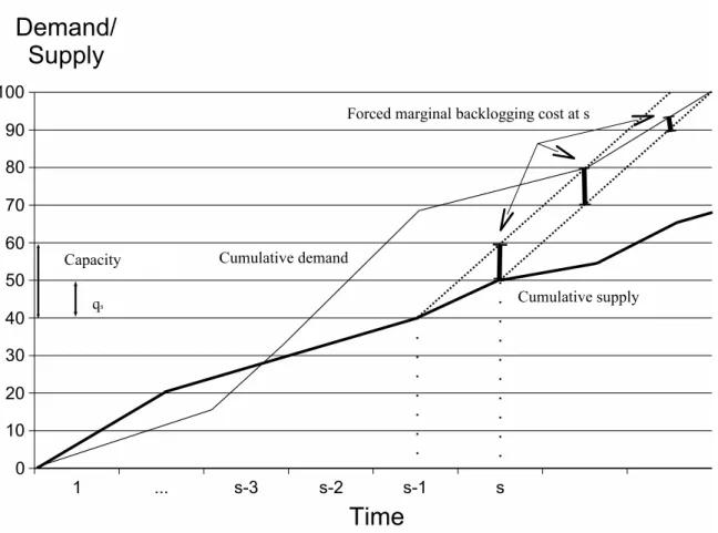
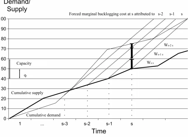
Figure 2 Forced marginal backorder cost accounting
Figures 1, 2 and 3 illustrate graphically the difference between classical period-by-period account-ing and forced marginal accountaccount-ing for backloggaccount-ing costs. All three figures reflect a saccount-ingle sample path of demands and orders. The total backlogging cost over the horizon is the area above the cumulative supply curve (thick line) and below the cumulative demand curve (thin line). Classical period-by-period accounting assigns to periods the difference between the curves ats(see Figure 1). Forced marginal accounting of backlogging costs assigns to periodsall of the backlogging costs that were ”forced”, or made inevitable, because we did not order to capacity in period s. This corresponds to the area inside of the trapezoid shown in Figure 2. This trapezoid is created by extending the cumulative supply curve, starting at s−1 and at s, to the right at a slope equal to the capacity of the system. These lines represent what the supply curves would look like if our policy consistently ordered at full capacity froms−1 andsonwards, respectively. In fact, consider the thick short bars in the trapezoid in Figure 2. The first and second terms of (2) are the vertical coordinates of the end points of these bars. Consequently eachWst, fort > s, is the length of one
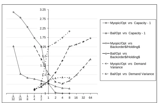
of these bars. Figure 3 takes a different point of view. It considers the backlogging costs incurred in periods, and illustrates how those costs are allocated to periods s, s−1, . . . ,1, . . . ,−L.
In Levi et al. (2007) it is shown that the marginal holding cost consists of a sum of partial expectations. Once xs is known at time s, the summands are expectations of simple piecewise
linear functions. If the accumulated demand D[s,j] (for eachj,s) has any of the distributions that are commonly used in inventory theory (e.g., Normal, Gamma, Lognormal, Laplace, etc) (Zipkin 2000), then it is extremely easy to evaluate these terms. If the distribution ofD[s,j]is discrete, these functions can be computed recursively in efficient ways using the CDF functions. More generally, the
Figure 3 Allocation of a period backorder to ordering decisions
complexity of evaluating the marginal holding cost can vary depending on the level of information we assume on the demand distributions and their characteristics. In all of the common scenarios there exist straightforward methods to solve this problem efficiently (see also Hurley et al. (2006) for more details). Since in the presence of positive lead times, even computing a simple Myopic policy requires the same knowledge on the distribution of the accumulated demand over the lead time, the computational effort involved with computing the marginal holding cost is of the same order of magnitude as for the Myopic policy. Evaluating the marginal backlogging costs based on the scheme developed in this paper is analogous to the marginal holding cost. It is a sum of partial expectations of simple piecewise linear functions, and therefore, is no more difficult to compute.
Finally, observe that for uncapacitated models with us=∞ for eachs (and hence ¯qs=∞), our
backlogging cost accounting is in fact identical to the traditional backlogging accounting discussed above. This implies that the cost accounting scheme proposed in this paper is a generalization of the one introduced in Levi et al. (2007). Therefore, the preceeding discussion is also a generalization of the corresponding algorithm and analysis in Levi et al. (2007).
4. Dual-Balancing Policy
In this section, we describe a new policy for the capacitated periodic-review stochastic inventory control problem. As in Levi et al. (2007), we call it a Dual-Balancing policy. We shall show that this policy has a worst-case performance guarantee of 2, i.e., for each instance of the problem, the expected cost of the policy is at most twice the expected cost of an optimal policy. Recall the assumption discussed in Section 2 that the cost parameters imply no motivation for holding inventory or backorders. This implies that, without loss of generality, for each t= 1, . . . , T, ct= 0
andht, pt≥0. Moreover, we first describe the algorithm, its analysis, and several extensions, under
The Dual-Balancing policy presented in this paper is based on a balancing idea similar to the one used in Levi et al. (2007) for the uncapacitated model. That Dual-Balancing policy balances, in each periodsand conditioned on the observed information setfs, the expected marginal holding
cost of the units ordered in the period against the expected (traditional) backlogging cost in period s+L, a lead time ahead of s. However, it is readily seen that this approach does not work in the case where there is a capacity constraint on the size of the order in period s. For one, the order sizeq0
s that balances these two costs might not be reachable when q0s> us.
In turn, we consider the forced marginal backlogging cost accounting and the corresponding cost it associates with period s as described in Section 3 above. Conditioned on the observed information set fs, we now balance the expected marginal holding cost of the units ordered in
periodsagainst the expectedmarginalbacklogging costs associated with periods. We will use the superscript B to refer to the Dual-Balancing policy. For each periods= 1, . . . , T−L, conditioning on the observed information setfs, let lBs(qsB) be the expected holding cost incurred over [s, T] by
the units ordered by the Dual-Balancing policy in period s. That is, lB
s(qsB) :=E[HsB(qsB)|fs]. In
Section 3 we have definedHB s =
PT
j=s+Lhj(QBt − (D[s,j]−XsB)+)+ (recall that we assumecs= 0).
In addition, let ˜πB
s :=E[ ˜ΠBs(qBs)|fs] be the expected backlogging cost associated with period s by
the forced marginal backlogging cost accounting scheme described above, again conditioned on the observed information setfs. Recall that in Section 3 we have defined ˜ΠBs =
PT t=s+LptWstB where, WB st = min{Q¯Bs, (D[s,t]−(XsB+QBs + X j∈(s,t] uj))+}= (D[s,t]−(XsB+QBs + X j∈(s,t−L] uj))+−(D[s,t]−(XsB+ X j∈[s,t−L] uj))+.
Since if we condition on fs, the inventory position at the beginning of period s, xBs, is known
deterministically; it is clear that lB
s(qsB) and ˜πsB(qBs) are both indeed functions ofqBs, the number
of units ordered in period s.
We first discuss the case where the orders are allowed to be fractional. This implies that the functions lB
s(qsB) and ˜πsB(qBs) are continuous. In each period s= 1, . . . , T−L, given the observed
information set fs, the Dual-Balancing policy will order qsB=qs0 ≤us units such that the expected
marginal ordering and holding cost incurred by these units over [s, T] is equal to the expected forced marginal backlogging cost associated with period s. In other words, we order q0
s units such
that lB
s(q0s) =E[HsB(qs0)|fs] = ˜πsB(qs0) =E[ ˜ΠsB(q0s)|fs]. Next we show that this policy is well-defined.
It is readily verified thatlB
s(qsB) is a convex increasing function ofqsB that is equal 0 forqsB= 0 and
goes to ∞ asqB
s goes to ∞. Similarly, one can verify that ˜πsB(qBs) is a decreasing convex function
of qB
s that has a non-negative value atqsB= 0 and that is equal to 0 for qsB=us (in this case there
is no unused slack capacity ats and ¯qB
s = 0). Our assumption that these functions are continuous
implies thatq0
s, as defined above, always exists.
Computationally, q0
s is the minimizer of the functiongs(qsB) := max{lBs(qsB),π˜Bs(qsB)}, which is a
convex function of qB
s, since it is the maximum of two convex functions. Hence, in each period s,
we need to solve a convex minimization problem of a single variable. In particular, if for eachj≥s, D[s,j] is distributed according to any of those distributions that are commonly used in inventory theory, then it is extremely easy to evaluate the functionslB
s(qsB) and ˜πsB(qBs). More generally, the
complexity of the algorithm is of order T (i.e., number of time periods) times the complexity of solving the single variable convex minimization defined above. The complexity of this minimization problem can vary depending on the level of information we assume on the demand distributions and their characteristics. In all of the common scenarios there exist straightforward methods to solve this problem efficiently. In particular, q0
s is determined by the intersection of two monotone
convex functions, which suggests that bisection methods can be effective in computingq0
that the Dual-Balancing policy is not a state-dependent base stock policy. However, it can be computed in anon-linemanner, i.e., computing the policy action in periodsdoes not require any knowledge on the future decisions to be made in the next periods. Moreover, unlike the Myopic policy, the Dual-Balancing policy does use available information about long term future demands.
4.1. Analysis
Next we show that, for each instance of the problem, the expected cost of the Dual-Balancing policy described above is at most twice the expected cost of an optimal policy. We will use the marginal cost accounting scheme described in Section 3 and amortize the period cost of the Dual-Balancing policy with the cost of the optimal policy.
Using the marginal cost accounting scheme discussed in Section 3, the expected cost of the Dual-Balancing policy can be expressed asE[C(B)] =PtT=1−LE[HB
t + ˜ΠBt ]. For each t= 1, . . . , T−L, let Ztbe therandom balanced costby the Dual-Balancing policy in periodt, i.e.,Zt=E[HtB|Ft]. Note
that Zt is a function of the observed information set in period t. In the next lemma we obtain an
expression for the expected cost of the Dual-Balancing policy using theZt variables. The proof is
identical to the proof of Lemma 4.1 in Levi et al. (2007).
Lemma 1. The expected cost of the Dual-Balancing policy is equal to twice the expected sum of the
Zt variables, i.e., E[C(B)] = 2
PT−L
t=1 E[Zt].
In the next two lemmas we show that the cost of OP T can be amortized against some of the cost of the Dual-Balancing policy. In particular, they imply that the expected cost ofOP T is at least PTt=1−LE[Zt]. For each realization of the demands D1, . . . , DT, let TH be the set of periods t= 1, . . . , T−L in which the optimal policy had inventory position higher than that of the Dual-Balancing policy, i.e., the set of periods 1≤t≤T−L such that YB
t < YtOP T. Let TΠ be the set of period in which the Dual-Balancing had inventory position at least as high as that ofOP T, i.e., the set of periodst= 1, . . . , T−Lsuch thatYB
t ≥YtOP T. (We consider only the periodst= 1, . . . , T−L,
because the effective ordering decisions are made in these periods. Specifically, each order placed after periodT−Lwill arrive after periodT.) Observe thatTH and TΠ are random sets that induce a random partition of the horizon.
The next lemma shows that, with probability 1, the marginal holding cost incurred by the Dual-Balancing policy in periods t∈ TH is at most the overall holding cost incurred by OP T, denoted
byHOP T, i.e.,P t∈THH
B
t ≤HOP T with probability 1. The proof is identical to the proof of Lemma
4.2 in Levi et al. (2007).
Lemma 2. For each realization fT ∈ FT, the total marginal holding cost incurred by the Dual-Balancing policy for all of the periods t∈ TH is at most the overall holding cost incurred by OP T, denoted by HOP T, i.e.,P
t∈THH B
t ≤HOP T with probability 1.
The next lemma shows that, with probability 1, the marginal backlogging cost of the Dual-Balancing policy associated with periodst∈ TΠis at most the overall backlogging penalty incurred by OP T, denoted by ˜ΠOP T.
Lemma 3. For each realizationfT∈ FT, the total marginal backlogging cost of the Dual-Balancing policy associated with all of the periods t∈ TΠ is at most the overall backlogging penalty incurred
byOP T, denoted by Π˜OP T, i.e.,P t∈TΠ
˜ ΠB
t ≤Π˜OP T with probability 1.
T he forced marginal backlogging cost associated with the periods inTΠ is equal to
X s∈TΠ X t:t≥s+L ptWstB= X t pt X s∈TΠ:s≤t−L WB st.
Therefore, it is sufficient to show that for each t=L+ 1, . . . , T, the traditional backlogging cost incurred by OP T in that period is at least as much as the forced backlogging costs incurred by the Dual-Balancing policy in periodt as a result of decisions made in periods{s∈ TΠ:s≤t−L}. In other words, it is sufficient to show that for eacht=L+ 1, . . . , T, we have
(Dt−N ItOP T)+≥
X
s∈TΠ:s≤t−L
WB
st,
with probability 1. (Recall that the backlogging costs over the periods 1, . . . , Lare the same for all policies.)
Consider now a specific realization fT ∈ FT and some period t= 1, . . . , T. If there is no period
in {s∈ TΠ:s≤t−L} with wBst>0, then there is nothing to prove. Assume that such a periods
exists, and let sl and se be, respectively, the latest and the earliest periods in the set
{s∈ TΠ:s≤t−L, wstB>0}, respectively (it is possible that sl=se). We note again that here we
abuse our notation and consider the set TΠ as the realized set of periods according to the specific realization fT. In particular, se and sl are the respective realizations of random variables Se and Sl. We have already seen (in the discussion in Section 3) that for eachs∈(se, sl] we havewstB= ¯qBs,
and wB se,t≤d[se,t]−(xse+qsBe+ P j∈(se,t−L]uj). Indeed, dt−niOP Tt =dt−(ysOP Tl + X j∈(sl,t−L] qOP T j −d[sl,t))≥d[sl,t]−(y B sl+ X j∈(sl,t−L] uj) =d[sl,t]−(y B se+ X j∈(se,sl] qB j −d[se,sl)+ X j∈(sl,t−L] uj) =d[se,t]−(x B se+q B se+ X (se,t−L] uj) + X j∈(se,sl] ¯ qB j ≥ X j∈[se,sl] wB st≥ X j∈[se,sl]∩TΠ wB st.
The first equality is based again on the fact that for each feasible policy and for each s≤t, we have N It=Ys+
P
j∈(s,t−L]Qj−D[s,t), applied to OP T and periods sl≤t−L. The first inequality
follows from the assumption that sl∈ TΠ and so yOP Tsl ≤y B
sl, and from the capacity constraints
that imply qOP T
j ≤uj. The second equality follows from the fact that (for each s≤s0) Ys0 = Ys+
P
j∈(s,s0]Qj−D[s,s0)applied to the Dual-Balancing policy and periodsse≤sl. The last equality is achieved by adding and subtractingPj∈(se,s
l]q¯ B
j and from the fact thatuj=Qj+ ¯Qj. The proof
then follows.
As a corollary of Lemmas 1, 2 and 3 we get the following theorem.
Theorem 2. The Dual-Balancing policy has a worst-case performance guarantee of 2, i.e., for each instance of the capacitated periodic-review stochastic inventory control problem, the expected cost of the Dual-Balancing policy is at most twice the expected cost of an optimal solution, i.e.,
E[C(B)]≤2E[C(OP T)].
F rom Lemma 1, we know that the expected cost of the Dual-Balancing policy is equal to twice the expected cost of the sum of the Zt variables, i.e., E[C(B)] =
PT−L
t=1 E[Zt]. From Lemmas 2
and 3 we know that, with probability 1, the cost of OP T is at least as much as the holding cost incurred by units ordered by the Dual-Balancing policy in periodst∈ TH plus the forced marginal
backlogging cost of the Dual-Balancing policy that is associated with periodst∈ TΠ. In other words, with probability 1,HOP T+ ˜ΠOP T ≥P t∈THH B t + P t∈TΠ ˜ ΠB
t . Using again conditional expectations
E[C(OP T)]≥E[X t∈TH HB t + X t∈TΠ ˜ ΠB t] = X t E[HB t ·11(t∈ TH) + ˜ΠBt ·11(t∈ TΠ)] = X t E[E[HB t ·11(t∈ TH) + ˜ΠtB·11(t∈ TΠ)|Ft]] = X t E[(11(t∈ TH) + 11(t∈ TΠ))Zt] = X t E[Zt].
We note that if the optimal policy is deterministic (i.e., it makes deterministic decisions in each periodt given the observed information setft), then if we condition onFt, then yBt and ytOP T are
known deterministically, and so are the indicators 11(t∈ TH) and 11(t∈ TΠ). If the optimal policy
is random, then the same arguments above still work. We now need to condition not only on Ft
but also on the decisions made by the policies. Since the inventory control policy does not have any effect on the evolution of the demand, the arguments above are still valid. This concludes the proof of the theorem.
We note that the examples discussed in Levi et al. (2007) show that the above analysis is tight. However, the analysis hints that in a typical scenario, the performance would be significantly better. Hurley et al. (2006) present a thorough empirical analysis of the typical performance of Dual-Balancing policies in uncapacitated models. In Section 6, we present empirical results that confirm that this phenomenon extends to the capacitated case.
Finally, we note that the Dual-Balancing policies and the worst-case analysis can be extended to models where the capacities in each period are generated by some exogenous random process, and the exact capacity available in period tis observed only at the beginning of the period. Thus, the Dual-Balancing policies provide a worst-case guarantee of 2 for this important extension as well. In this case, the expectations of the marginal backlogging costs are taken with respect to both the random future demands and random future capacities. In Appendix C, we consider two extensions of the Dual-Balancing policy and the worst-case analysis. Specifically, we discuss the extensions to models where orders must be integral and the demands are integer-valued random variables, and to models with stochastic lead times under the no order crossing assumption.
4.2. Cost Transformation
In this section, we discuss in detail the cost transformation that enables us to assume, without loss of generality, that for each periodt= 1, . . . , T, we havect= 0 andht, pt≥0. Consider any instance
of the problem with cost parameters that imply no speculative motivation for holding inventory or backorders (as discussed in Section 2). Following Levi et al. (2007), we use a simple transformation of the cost parameters to construct an equivalent instance, with the property that for each period t= 1, . . . , T, we havect= 0 andht, pt≥0. More specifically, the modified instance has the same set
of optimal policies. Applying the Dual-Balancing policy to that instance, we obtain a policy that is different from the original dual balancing policy, and which also has a performance guarantee of at most 2 with respect to the original problem. We shall show that this cost transformation can improve the performance guarantee of the Dual-Balancing policy in cases where the ordering cost is the dominant part of the overall cost. In practice this is often the case.
We now describe the transformation for the case with no lead time (L= 0) and α= 1; the extension to the case of arbitrary lead time is straightforward. Recall that any feasible policy P satisfies, for eacht= 1, . . . , T,Qt=N It−N It−1+Dt (for ease of notation we omit the superscript P). Using these equations, we can express the ordering cost in each periodtasct(N It−N It−1+Dt).
Now replaceN It with N It+−N It−, its respective positive and negative parts.
This leads to the following transformation of cost parameters. We let ˆct:= 0, hˆt:=ht+ct− ct+1(cT+1= 0) and ˆpt:=pt−ct+ct+1. Note that the assumptions on the cost parametersct, ht,and ptdiscussed in Section 2, and in particular, the assumption that there is no speculative motivation
that the parameters ˆht and ˆbt will still be non-negative even if the parameters ct, ht, and pt are
negative and as long as the above assumption holds. Moreover, this enables us to incorporate into the model a negative salvage cost at the end of the planning horizon (after the cost transformation we will have non-negative cost parameters). It is readily verified that the induced problem is equivalent to the original one. More specifically, for each realization of the demands, the cost of each feasible policy P in the modified input decreases by exactlyPTt=1ctdt (compared to its cost
in the original input). Therefore, any optimal policy for the modified input is also optimal for the original input.
Now apply the Dual-Balancing policy to the modified problem. We have seen that the assump-tions onct, htandptensure that ˆhtand ˆptare non-negative and hence the analysis presented above
is valid. Letopt and opt be the optimal expected cost of the original and modified inputs, respec-tively. Clearly,opt=opt+E[PTt=1ctDt]. Now the expected cost of the Dual-Balancing policy in the
modified input is at most 2opt. Its cost in the original input is then at most 2opt+E[PTt=1ctDt] =
2opt−E[PTt=1ctDt]. This implies that if E[
PT
t=1ctDt] is a large fraction of opt, then the perfor-mance guarantee of the expected cost of the Dual-Balancing policy might be significantly better than 2. For example, if E[PTt=1ctDt]≥0.5opt, then we can conclude that the expected cost of the
Dual-Balancing policy is at most 1.5opt. It is indeed the case in many real life problems that a major fraction of the total cost is due to the ordering cost. The intuition of the above transforma-tion is that PTt=1ctDt is a cost that any feasible policy must pay. As a result, we treat it as an
invariant in the cost of any policy and apply the approximation algorithm to the rest of the cost. In the case where we have a lead time L, we use the equationsQt:=N It+L−N It+L−1+Dt+L,
for each t= 1, . . . , T −L, to get the same cost transformation. The transformation for α >1 is also straightforward. Also, it is not hard to see that the cost transformation can be modified to remove, say, γ% of the per-unit ordering costs, where 0< γ <100. This leads to a continuum of dual balancing policies, all of which are 2-approximations.
5. Improved Policy & Bounds on the Optimal Inventory Levels
In this section, we consider two semi-myopic (modified) base-stock policies that are easy to compute in an on-line manner and provide, respectively, lower bounds and upper bounds on the inventory levels of an optimal policy yOP T
t , in each period t= 1, . . . , T. We believe that these bounds can
be used effectively to improve existing algorithms for computing inventory control policies for the capacitated model discussed in this paper and other capacitated stochastic inventory models. Moreover, as in Hurley et al. (2006), we shall show that these policies provide bounds that are strong in the following sense: each policy that, for some period t and some stateft, has inventory level
outside the range defined by the respective lower and upper bounds can be improved. In particular, there is another (modified) policy that in period t and state ft, admits an inventory level within
the specified range, with expected cost no greater than the expected cost of the original policy. In other words, any policy that violates these respective bounds is dominated by another policy. We then follow Hurley et al. (2006) and construct anImproved Dual-Balancing policythat incorporates these bounds. This policy also has a performance guarantee of 2 and as the computational study for the uncapacitated model in Hurley et al. (2006) suggests, we expect that it will have a better typical performance.
The policies we consider are calledLower-Myopic(denoted byLM) andUpper-Myopic(denoted by U M), respectively. In the Lower-Myopic policy, in each periods, conditioning on the observed information setfs, we minimize thesumof the expected marginal holding cost of the units ordered
in that period and the traditional expected backlogging costs a lead time ahead. That is, in each periods, we minimize
gLM
under the constraint qs≤us. This is a convex function of qs. This policy has been first proposed
for the uncapacitated model by Levi et al. (2007) who called it the Minimizing policy. They have shown that this is a base-stock policy that provides lower bounds on the optimal base-stock levels. However, in the capacitated model it is possible that the actual minimizer will not be attainable. In this case we order up to capacity, and this provides a modified base-stock policy. In this paper, we extend and generalize their proof for the capacitated model. In the Upper-Myopic policy, in each periods, again conditioning on fs, we minimize the sum of the expected period holding cost
and the expected forced marginal backlogging. Thus, we minimize gU M
s (qs) = ˜πU Ms (qs) +E[hs+L(xs+qs−D[s,s+L])+|fs],
subject to 0≤qs≤us, which is also convex in qs. We shall show that this policy provides upper
bounds on the inventory levels of an optimal policy. By arguments similar to the ones used by Levi et al. (2007), it can be shown that this gives rise to yet another modified base-stock policy. (In particular, gU M
s (q1)−gU Ms (q2) depends only on y1=xs+q1 and y2=xs+q2.) To the best of our
knowledge, this is a new way for deriving upper bounds on the inventory levels of an optimal policy in the capacitated model. We note that it is not clear whether the classical Myopic policy, where we minimize the expected period cost, provides any bounds for capacitated models. Another similar open question is how the policy that in each period minimizes the sum of the expected marginal holding cost and expected forced marginal backlogging cost is related to an optimal policy.
Let YLM
t and YtU M be the respective inventory position (after orders are placed) of the
Lower-Myopic and the Upper-Lower-Myopic policies in periodt= 1, . . . , T. Specifically, we assume thatYLM t is
the smallest minimizer of the corresponding period problem being solved (see above) and thatYU M t
is the largest minimizer of the corresponding period problem. Note that the inventory position levels depend on the specific state (ft, xt), but for ease of notation we omit the indication of the
state. The two semi-myopic policies described above can be implemented in an on-line manner, i.e., regardless of the action control in future periods. We shall show that for each evolution fT,
these two policies provide lower and upper bounds on the inventory levels of any optimal policy, i.e., YLM
t ≤YtOP T ≤YtU M, with probability 1, for each t= 1, . . . , T. Moreover, we shall show that
each non-dominated policy P must have YLM
t ≤YtP≤YtU M, for eacht= 1, . . . , T.
The next two lemmas show that each policyP that has, for some periodsand statefs, inventory
position yP
s ∈/[ysLM, ysU M], can be strictly improved by a modified policy P0 with yP
0
s ∈[ysLM, ysU M]
and expected cost at most the expected cost of P. For the sake of simplicity, we consider a model with no lead time (the extensions to the case withL >0 are straightforward).
Lemma 4. Consider a feasible policy P, and suppose that for some period s and information set
fs, we have ysP < ysLM. Further assume that s is the earliest such period. Then the policy P0 that follows P until period s−1, then orders up to yLM
s in period s and again imitates P over the interval (s, T], has expected cost no larger than the expected cost of P.
S ince P0 follows P over [1, s), we conclude that they incur exactly the same cost over that
interval, and that they have the same inventory position xs≤yPs < yLMs . Since s is the first such
period, we conclude thatP0 can indeed order up toyLM
s . Now over (s, T],P0 imitatesP; that is, it
orders nothing ifXP0
j ≥YjP and orders up toYjP otherwise (for eachj∈(s, T]). Moreover, the policy P0 has ordered qP0
s units in periods. Consider the overall expected marginal holding cost of these
units and the expected (traditional) backlogging cost incurred byP0 in periods. By the definition
of qP0
s , it is clear that this is no greater than the expected marginal holding cost and expected
(traditional) backlogging cost incurred by the policy P in period s. For each period j∈(s, T], we know that with probability 1, YP0
j ≥YjP and that QP
0
j ≤QPj. This implies that the backlogging
incurred by policy P0 over that interval is no greater than the backlogging cost incurred by policy
P, and similarly, the marginal holding cost policy P0 incurs over that interval is no greater than