Velocity Modeling in a Vertical Transversely Isotropic
Medium Using Zelt Method
Maryam Sadrii*, H.R.Ramaziii and M. Ali Riahiiii
i * Corresponding Author, Maryam Sadri, Ph.D. Student of Mining Engineering, Dept. of Mining, Metallurgy and Petroleum Engineering, Amirkabir University of Technology, Tehran, Iran ([email protected]).
ii H.R Ramazi, Assistant Professor, Dept. of Mining, Metallurgy and Petroleum Engineering, Amirkabir University of Technology, Tehran, Iran. iii M. Ali Riahi, Associate Professor, Institute of Geophysics, University of Tehran, PO Box 14155-6466, Tehran, Iran.
Received 05 July 2008; received in revised 12 January 2009; accepted 14 February 2009 ABSTRACT
In the present paper, the Zelt algorithm has been extended for ray tracing through an anisotropic model. In anisotropic media, the direction of the propagated energy generally differs from that of the plane-wave propagation. This makes velocity values to be varied in different directions. Therefore, velocity modeling in such media is completely different from that in an isotropic media.
The velocity model for ray tracing is parameterized in terms of blocky trapezoid cells where the velocity changes inside the cells linearly. Thomsen’s approximations in weakly anisotropic media were used to estimate anisotropic velocity vectors. Rays were traced in direction of group vector in the vertical transversely isotropic (VTI) media, whereas, the anisotropic Snell’s law must be satisfied by the phase angle and phase velocities across the interface.
The synthetic examples are given to demonstrate and verify the ray tracing algorithm. Reflected and turning waves were traced through the isotropic and anisotropic velocity models. Lateral and vertical velocity variation caused deviation on trajectory of the traveltime curve.
The results show that the difference between isotropic and anisotropic traveltimes increases with offset, especially when the ratio offset/depth exceeds 1.5.
KEYWORDS
Ray tracing, Vertical Transversely Isotropy (VTI), Zelt method, seismic velocity modeling.
1. INTRODUCTION
In a homogenous anisotropic medium, the wave behavior is quite different from that in isotropic media (Helbig, 1994) and the velocity of a seismic wave changes with the direction of propagation. Parallel cracks, stratified layering, orientation of grains and rock foliation cause velocity anisotropy (Postma, 1955; Krey and Helbig, 1956; Levin, 1978; Berryman, 1979; Helbig, 1981; Schoenberg, 1983; Thomsen, 1986).
There are different ray tracing methods to model the velocity distribution. Shooting or bending algorithms are generally used to trace the ray path from a source point to a receiver (Julian and Gubbins, 1977). Cerveny (1985) applied paraxial extrapolation to estimate the traveltimes. Finite-difference methods were used by Reshef and Kosloff (1986), Vidale (1988), Podvin and Lecomte (1991), and Van Trier and Symes (1991) to estimate the first arrival traveltimes. Moser (1991) presented a graph
theory to calculate the shortest ray path between source and receiver. Vinje et al. (1993) and Lomax (1994) simulated the wave fronts instead of ray paths.
Zelt and Ellis (1988) presented a ray tracing algorithm in a 2-D isotropic velocity model. The model is divided by a series of trapezoidal blocks in each layer. The velocity within the trapezoidal cell is defined linearly. Zelt and Smith (1992) introduced a method of seismic traveltime inversion for determination of 2-D velocity model and interface structure. The ray tracing algorithm was a modification of that presented by Zelt and Ellis (1988). They defined velocity nodes for the corners of the trapezoid. Zelt (1999) applied seismic refraction/wide-angle reflection traveltimes to obtain 2-D velocity model and interface structure.
on ray tracing in an anisotropic model. Thomsen’s (1986) approximations for weakly anisotropic media were used to estimate the anisotropic velocity vectors. Slawinski et al.’s (2000) equations for horizontal anisotropic media were extended in a dipping anisotropic layering model to compute the ray direction. The main advantages of this method are simplicity and minimum number of parameters needs to define the model. This method is suitable for multi-shot recording to define optimal geometry of receivers in seismic operation planning. 2. VELOCITY MODEL
In anisotropic media, the traveltime function is governed by an advanced form of the eikonal equation. Solution of this equation by the method of ray tracing is discussed by Cerveny et al. (1977). The kinematic ray tracing calculations were performed by solving the ray tracing system (Cerveny et al., 1977).
In this study, the earth model was supposed to be homogenous and isotropic/anisotropic composed of a sequence of layers. Each layer is divided into trapezoidal cells (Fig.1). The interface of layers is specified by an arbitrary number of boundary nodes connected by linear interpolation. The number and position of the nodes may differ for each interface. The P-wave velocity within the trapezoidal cell is described as follows (Zelt and Smith, 1992):
(1)
( )
(
(
)
)
7 6
5 4 3 2 2 1
,
c x c
c xz c z c x c x c z x V
+
+ + + + =
where, ci is linear combination of the corner velocities (V1,V2,V3and V4).
In the case of P-wave propagation in VTI (vertically transverse isotropy) media, velocity determination requires the estimation of three parameters; Vp0(P-wave
velocity in the direction of the symmetry axis), ε (fractional difference between velocities perpendicular and parallel to bedding), and δ (the variation in P-wave velocity close to the symmetry axis). Under the assumption of weak anisotropy (ε <<1,δ <<1), the Thomsen (1986)’s approximation for P-wave phase velocity is:
(2)
( )
θ(
δ 2θ 2θ ε 4θ)
01+ sin cos + sin
= p
p V
V
where, Vp
( )
θ is the phase velocity in the phase angle θmeasured from the vertical axis of symmetry.
The Thomsen anisotropic parameters must be defined for each velocity nodes (Fig.1).
Figure 1: The corner parameters of the cell in an anisotropic model: εiand δi are Thomsen anisotropic parameters; Viis the vertical velocity.
3. RAY TRACING
In anisotropic media, the direction of the propagated energy (group vector) generally differs from that of the plane-wave (phase vector). Therefore, the ray angle Φ is different from the phase angle θ except at φ=θ=0 and
2
Π
(Fig.2).
Figure 2: Relationship between velocity vectors in an anisotropic model. V (θ): phase velocity; V (Φ): group velocity; θ: phase angle; Φ: group angle.
Shooting method is applied to trace rays through the 2-D velocity model. Ray tracing is carried out by numerical solving of the two dimensional ray tracing equations by Cerveny et al., (1977):
(3)
(
)
V V V
dz d dz dx
x
z −
= =
θ θ
θ
tan tan
where, θ is the angle between velocity vector and z-axis,
Vis the velocity of a cell (equation 1), and Vx and Vz are partial derivatives of velocity with respect to x and z direction.
The rays are traced with P-wave group vector through the model, whereas the Snell’s law should be satisfied across the interface with phase angle and phase velocities:
(4) )
( sin ) ( sin
2 2 1
1
θ θ θ
θ
p
p V
V =
(5)
(
) (
)
(
) (
)
tan 1 ( ) .
tan
1 tan . 1 ( ) . i
i
i
V dV d
V dV d
θ
θ
θ
ϕ
θ
θ
θ
+ = −where, φiis the take-off angle. In this paper, the subscripts i and t refer to the medium of incidence and transmission, respectively.
Once the phase angle,θi, is found, the ray parameter, x0 , can be calculated as:
(6) ) sin cos . sin 1 ( sin 4 2 2 0 0 i i i i i i i V x θ ε θ θ δ θ + + =
Equation (7) can be solved for the transmitted phase angle (θt):
(
)
(
V0tx0εt−δt)
sin4θt+(
V0tx0.δt)
sin2θt−sinθt+(
V0t.x0)
=0(7). The transmitted group angle,φt, which the group
velocity vector makes with the normal to the interface, can be calculated based on the transmitted phase angle,θt, from equation (8), (Slawinski et al., 2000):
(8)
(
)
( )
( )
( )
[
(
)
]
⎥⎥ ⎥ ⎥ ⎥ ⎦ ⎤ ⎢ ⎢ ⎢ ⎢ ⎢ ⎣ ⎡ − + − − = − 2 2 0 2 2 0 1 cos 2 2 cos 2 sin . 1 sin cos 2 2 cos . 2 sin cos cos t t t t t t t t t t t t t t t t t V r r V ξ ε ξ δ ξ ξ ξ ξ ξ ε ξ δ ξ ξ φwhere,ξt is the phase latitude (ξt =90−θt), and
(9)
( )
(
2 2 4)
0
1
1 sin .cos cos
t t
t t t t t
r V
ξ
δ
ξ
ξ ε
ξ
= + +The traveltime at the endpoint of the ray is estimated by numerical integration along the ray path (Eq. 10). By linear interpolation across the endpoints of the two closest rays that surround the point of interest, the traveltime associated with a specific receiver location is determined.
(10)
∑
=
= n
i Vi
d t
1
where, t is traveltime, d is ray step length, and Viis the ray velocity.
4. SYNTHETIC EXAMPLES
Methodology examination accomplished by the computer program was written for ray tracing in 2-D isotropic and anisotropic media. To test the algorithm, a velocity model consisting of 7 layers was defined. The velocity model with isotropy/anisotropy parameters and
reverse fault which has interrupted the horizontal layers. The fault is terminated in 2nd layer and continued to the 5th
layer.
A. A homogenous-isotropic model
To start the ray tracing, we assumed a homogeneous isotropic condition for 2D velocity model. In this model, the velocity in each layer was supposed to be constant. The 5th layer has the lower velocity than the upper layers.
Therefore, the strong reflection surface is made at the top of this layer. Table 1 shows the velocity values for the model.
TABLE 1
PARAMETERS FOR THE HOMOGENOUS-ISOTROPIC VELOCITY MODEL.
layer Vp0 (m/s) 1 1800 2 2500 3 2000 4 3500 5 2700 6 3500 7 3000
Rays were traced through the model by the new method. The ray paths and corresponding synthetic sections are plotted in Fig.3. The synthetic seismograms were produced by convolution of traveltimes with 60 Hz Ricker wavelet. The amplitude is the same for all traces. Figure 3a shows the reflected rays from the second layer (the shot is located on x=8 km).
The shot location moved to x=12.5 km and the ray tracing carried out on the 5th layer (Fig. 3b). Because of
the velocity contrast between 3rd and 4th layers, the critical
angel occurs at 34 degree on this interface. Therefore, the long offsets were missed on the 5th layer during the ray
tracing.
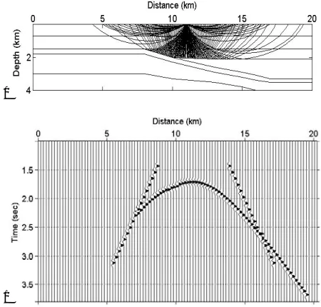
Ray tracing through the 6th reflector has been shown in
Fig.3c. The shot is located at x=12.5 km. Presence of the fault in this model was caused lateral velocity variation during the ray tracing on 6th layer. Velocity changes and
Figure 3: Reflected P-wave rays were traced trough the homogenous-isotropic media. Velocity model and reflected rays with related synthetic seismograms are shown for (a) second layer, (b) fourth layer, and (c) sixth layer.
B. A heterogeneous-isotropic model
Vertical velocity gradient is considered for the previous velocity model. Ray bending occurs when the vertical velocity changes within a trapezoidal cell. Table 2 shows the velocity gradients in each layer.
TABLE 2
PARAMETERS FOR THE HETEROGENOUS-ISOTROPIC VELOCITY MODEL.
layer Vp0 (m/s) vertical gradient
1 1800-2000 2 2400-2750 3 2900 4 3450-3900 5 3950-4200 6 4500 Due to vertical velocity gradient, turning waves were generated during ray tracing. Figure 4a shows the turning waves which travel in the curvature paths. The linear events in seismogram are related to the turning waves produced in the first layer (Fig. 4b). The unconformity located in the middle part of the section causes time distortions on the hyperbolic traveltime curve corresponded to the 3rd reflector.
Figure 4: (a) Reflected rays were traced on the bottom of the 3rd layer in the heterogeneous-isotropic media. (b) Linear events in seismogram are related to the turning waves generated in the first layer. The hyperbola is reflection curve of the 3rd layer.
(a)
(b) (b)
C. A homogenous-anisotropic model
The 2D-VTI model selected from Grechka and Tsvankin (2002) comprises the three homogenous layers. The parameters for the weak anisotropic model have been shown in Table 3, where ε and δ are Thomsen parameters for a VTI medium.Vp0is the vertical p-wave velocity. The velocities in each layer are assumed to be constant with different anisotropic parameters.
TABLE 3
PARAMETERS FOR THE WEAKLY ANISOTROPIC VELOCITY MODEL.
layer Vp0 (m/s) ε δ
1 2000 0.2 0.1
2 2500 0.25 0.05
3 3000 0.15 0.1
We traced the rays corresponding to the P-wave reflections from the source point located at 1850 m with different propagation angles to the bottom of the 3rd layer (Fig.5).
Figure 5: Reflected P-wave rays were traced trough the anisotropic media. The source point is located at x=1850 m.
All the rays should satisfy the anisotropic Snell’s low. The critical angle for the reflected rays is checked in each interface by solving the equation (7). Imaginary answers for this equation mean that the ray is unable to penetrate to the lower layers and should be reflected. The boundaries should be smoothed before raytracing because the features with abrupt dip could make shadow zones.
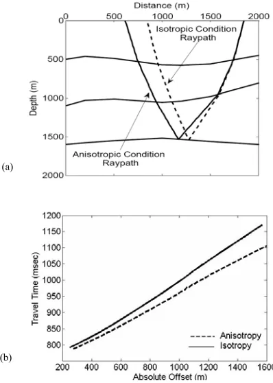
For testing the anisotropic effect, the ray tracing was performed through the model with isotropic assumption (ε=δ=0). Fig.6a shows the comparison of ray paths under isotropy and anisotropy conditions. It seems that the difference between the two ray paths is related to the anisotropic parameters. The difference between traveltimes computed from the isotropic and anisotropic models increases with offset. Anisotropic parameters cause the significant effects on the long offsets especially when the ratio offset/depth exceeds 1.5 (Fig.6b).
Figure 6: Comparison of isotropic and anisotropic ray tracing results (source point is located at x=1850 m). (a) Ray directions change in anisotropic layers, (b) the difference between traveltimes computed by the ray tracing through the isotropic and anisotropic models.
5. CONCLUSION
A new method of ray tracing based on Zelt and Ellis’s (1992) algorithm for vertical transversely isotropic media has been developed. The new method of ray tracing has been examined in different velocity models (isotropic/anisotropic). The main advantages of this method are simplicity and a minimum number of parameters needs to define the model. This method is suitable for multi-shot recording to define optimal geometry of receivers in seismic operation planning.
The synthetic data presented to test the method show that the difference between traveltimes computed from the isotropic and anisotropic model increases with offset. Anisotropic parameters cause significant effects on the long offsets especially when the ratio offset/depth exceeds 1.5.
6. ACKNOWLEDGMENT
It is necessary to thank Dr. C. Zelt from Rice University for sending his paper.
7. REFERENCES
[1] J.G. Berryman, “Long-wave elastic anisotropy in transversely isotropic media,” Geophysics, vol. 44, pp. 896-917, 1979. [2] V. Cerveny, I.A. Molotkov, and I. Psencik, Ray method in
seismology, Universita Karlova, 1977.
[3] V. Cerveny, The application of raytracing to the numerical modeling of seismic wavefields in complex structures, Handbook of geophysical exploration, Geophysical Press, London, 1985. [4] V. Grechka, I. Tsvankin, “PP+PS=SS,” Geophysics, vol. 67, pp.
1961-1971, 2002.
[5] K. Helbig, “Systematic classification of layer-induced transverse isotropy,” Geophy. Prosp., vol. 29, pp. 550-577, 1981.
[6] K. Helbig, Foundations of anisotropy for exploration seismic. Handbook of Geophysical Exploration. Oxford, Pergamon, 1994. [7] B.R. Julian, and D. Gubbins, “3-D seismic ray tracing,”
Geophysics, vol. 43, pp. 95-113, 1977.
[8] Th. Krey, K. Helbig, “A theorem concerning anisotropic stratified media and its significance for reflection seismic,” Geophy. Prosp., vol. 4, pp. 294- 302, 1956.
[9] F.K. Levin, “The reflection, refraction of waves in media with elliptical velocity dependence,” Geophysics, vol. 43, pp. 528- 537, 1978.
[10] A. Lomax, “Wavelength-smoothing method for approximating broad-band wave propagation through complicated velocity structures,” Geophysics. J. Int., vol. 117, pp. 313-334, 1994. [11] T. J. Moser, “Shortest path calculation of seismic rays,”
Geophysics, vol. 59, pp. 59-67, 1991.
[12] P. Podvin, and I. Lecomte, “Finite difference computation of traveltimes in very contrasted velocity models: a massively parallel approach and its associated tools,” Geophys. J. Int., vol. 105, pp. 271-284, 1991.
[13] G.W. Postma, “Wave propagation in a stratified medium,” Geophysics, vol. 20, pp. 780-806, 1955.
[14] M.Reshef, and D. Kosloff, “Migration of common-shot gathers,” Geophysics, vol. 51, pp. 324-331, 1986.
[15] M. Schoenberg, “Reflection of elastic waves from periodically stratified media with interfacial slip,” Geophys. Prosp., vol. 34, pp. 265-292, 1983.
[16] M.A Slawinski, A. Raphael, R. Slawinski, and B. James, “A generalized form of Snell’s law in anisotropic media,” Geophysics, vol. 65, pp. 632-637, 2000.
[17] L. Thomsen, “Weak elastic anisotropy,” Geophysics, vol. 51, pp. 1954-1966, 1986.
[18] J. Van Trier, and W.W. Symes, “Upwind finite difference calculation of traveltimes,” Geophysics, vol. 56, pp. 812-821, 1991.
[19] J. Vidale, “Finite-difference calculation of traveltimes,” Bulletin of the Seismological Society of America, vol. 78, pp. 2062-2076, 1988.
[20] V. Vinje, E. Iversen, and H. Gjoystdal, “Traveltime and amplitude estimation using wavefront construction,” Geophysics, vol. 58, pp. 1157-1186, 1993.
[21] C.A. Zelt, and R.M. Ellis, “Practical and efficient ray tracing in two-dimensional media for rapid traveltime and amplitude forward modeling,” Canadian Journal of Exploration Geophysics, vol. 24, pp. 16-31, 1988.
[22] C.A. Zelt, and R.B. Smith, “Seismic traveltime inversion for 2-D crustal velocity structure,” Geophys. J. Int., vol. 108, pp. 16-34, 1992.