University of New Orleans
University of New Orleans
ScholarWorks@UNO
ScholarWorks@UNO
University of New Orleans Theses and
Dissertations
Dissertations and Theses
Spring 5-18-2012
The Interacting Multiple Models Algorithm with State-Dependent
The Interacting Multiple Models Algorithm with State-Dependent
Value Assignment
Value Assignment
Rastin Rastgoufard
University of New Orleans, [email protected]
Follow this and additional works at: https://scholarworks.uno.edu/td
Part of the Artificial Intelligence and Robotics Commons, Signal Processing Commons, and the
Statistical Models Commons
Recommended Citation
Recommended Citation
Rastgoufard, Rastin, "The Interacting Multiple Models Algorithm with State-Dependent Value Assignment" (2012). University of New Orleans Theses and Dissertations. 1477.
https://scholarworks.uno.edu/td/1477
This Thesis is protected by copyright and/or related rights. It has been brought to you by ScholarWorks@UNO with permission from the rights-holder(s). You are free to use this Thesis in any way that is permitted by the copyright and related rights legislation that applies to your use. For other uses you need to obtain permission from the rights-holder(s) directly, unless additional rights are indicated by a Creative Commons license in the record and/or on the work itself.
The Interacting Multiple Models Algorithm with State-Dependent Value Assignment
A Thesis
Submitted to the Graduate Faculty of the University of New Orleans
in partial fulfillment of the requirements for the degree of
Master of Science in
Engineering Electrical
by
Rastin Rastgoufard
B.Sc. Tulane University, 2008
Acknowledgements
I had a lot of fun in the three and a half years of my master’s degree. For that, I would like to thankallof
the professors of UNO’s Department of Electrical Engineering and the students who were with me.
I would like to make special mention of the three professors in the Information Systems Lab: Dr. Jilkov,
Dr. Chen, and my advisor, Dr. Li. Your continuous instruction and encouragement shaped my coursework,
provided the path to my master’s thesis, and radically expanded the boundaries of my mind.
Contents
List of Figures iv
Abstract v
Introduction 1
Toy Problem . . . 1
Goals . . . 2
Brief Overview of Existing Literature . . . 5
Brief Overview of Proposed Methods . . . 7
Kalman Filter 8 Algorithm . . . 8
Small Visual Example . . . 9
Interacting Multiple Models 11 Step 1, Mix . . . 11
Step 2, Run Individual Filters . . . 12
Step 3, Remix . . . 14
Prediction . . . 14
Small Visual Example . . . 15
State-Dependent Value Assignment 18 A State’s Value . . . 18
SD Model Probabilities . . . 19
SD Transition Probabilities . . . 20
Small Visual Example . . . 21
Experiment and Results 23 Experimental Design . . . 23
Results . . . 26
Discussion 28 State-Dependent Performance . . . 29
State-Dependent Comparison . . . 30
The Value Function . . . 32
Conclusion 34 References 36 Appendices 37 Simulation Results . . . 37
Code Listing . . . 49
List of Figures
# Page
1 Vehicle passes beside two obstacles. . . 4
2 Vehicle enters an obstacle. . . 4
3 One entire player-controlled trajectory. . . 4
4 Another entire trajectory. . . 4
5 KF, One Step . . . 10
6 KF, One Step, Two Models . . . 10
7 A first step using the IMM algorithm. . . 17
8 A second step using the IMM algorithm. . . 17
9 IMM’s prediction for the third step. . . 17
10 The value functions(x), two differentβ. . . 19
11 SD TPM Example . . . 22
12 Mode sequences over two time steps. . . 24
13 Performance Summaries . . . 28
14 Truth and Predictions. . . 31
15 SD cases with good behavior. . . 31
16 SD MPs sometimes better than SD TPM. . . 33
17 Inaccurate TPM. . . 33
18 2011.10.17.11.36.22, 0.08 to 74.15 . . . 37
19 2011.10.17.11.36.22, 10.00 to 15.00 . . . 38
20 2011.10.17.11.36.22, 10.00 to 50.00 . . . 39
21 2011.10.17.11.36.22, 15.00 to 20.00 . . . 40
22 2011.10.17.11.36.22, 25.00 to 30.00 . . . 41
23 2011.10.17.11.36.22, 30.00 to 35.00 . . . 42
24 2011.10.17.11.36.22, 30.00 to 60.00 . . . 43
25 2011.10.17.11.36.22, 35.00 to 40.00 . . . 44
26 2011.10.17.11.36.22, 45.00 to 50.00 . . . 45
27 2011.10.17.11.36.22, 50.00 to 55.00 . . . 46
28 2011.10.17.11.36.22, 55.00 to 60.00 . . . 47
Abstract
The value of a state is a measure of its worth, so that, for example, waypoints have high value and regions
inside of obstacles have very small value. We propose two methods of incorporating world information as
state-dependent modifications to the interacting multiple models (IMM) algorithm, and then we use a game’s
player-controlled trajectories as ground truths to compare the normal IMM algorithm to versions with our
proposed modifications. The two methods involve modifying the model probabilities in the update step and
modifying the transition probability matrix in the mixing step based on the assigned values of different target
states. The state-dependent value assignment modifications are shown experimentally to perform better than
the normal IMM algorithm in both estimating the target’s current state and predicting the target’s next
state.
Introduction
Toy Problem
We created a “game” that allows the player to generate ground truth trajectories. The user controls a vehicle,
in real time, through a two-dimensional world which contains several obstacles, circular regions of varying
radii. The vehicle is not supposed to enter the obstacle regions as it navigates around. Consider Figures 1 to
4 for visual reference during the following explanation.
The vehicle itself is shown in blue. Theopen blue circleshows the location of the vehicle, and theblue
dotshows the direction that the vehicle is facing. The player controls both the direction of the vehicle, using
the left and right arrow keys, and the forward speed of the vehicle, using the space-bar key. In the game, the
vehicle’s rotation and forward speed are not coupled, meaning that the vehicle can rotate while stopped. The
maximum turn rate is constant regardless of the vehicle’s forward speed.
Theblack dotsindicate the boundary of an obstacle. In Figure 1, two obstacles are visible. One has a
large radius and is located up and to the left of the vehicle. The other is small and is centered at (2,2). In
the same figure, thesmall red Xshows where the center of the (2,2) obstacle is located.
The playing world contains a total of four obstacles. There is onesmall red dotfor each of the obstacles.
The location of each red dot is an indication of where each corresponding obstacle’s boundary is located with
respect to the vehicle. In Figure 1, there are two red dots immediately to the left of the vehicle that indicate
the vehicle is close to two obstacle boundaries. There is another red dot located up and to the right of the
vehicle that indicates there is a slightly distant obstacle in that direction. There is a final red dot below and
to the left of the vehicle that indicates there is an obstacle very far from the vehicle in that direction.
Figures 1 to 4 were created after the player controlled the vehicle for approximately 75 seconds. The
black line shows a sliding window of the vehicle’s trajectory. The green circlesshow snapshots of the
vehicle’s trajectory taken everyT = 0.35 seconds. Neither of these was visible to the player before the run
was completed, as both would have required knowledge of the future.
The player can drive the vehicle anywhere in the toy world. The obstacles do not have hard boundaries,
red dot. Figure 2 shows the vehicle inside of an obstacle. The position of the heavy red X with respect to the
vehicle shows the direction of the nearest exit point from the obstacle. If this toy world were a game that
distributed points, then the player would always choose to exit toward the heavy red X in order to minimize
the amount of points lost for being in an obstacle.
Goals
Three main goals form the basis for this thesis. It is important to use a real world target, to incorporate the
obstacle information into a tracking algorithm, and to track (both estimate and predict) the motion of that
target.
1. Real World Target
The vehicle that is controlled by the player behaves like a “real world” target. The target has a very wide
array of possible maneuvers, and the player can make decisions of how to move the target in real time.
This is in contrast with an algorithmically determined target that is often used in computer simulations.
This goal is important because a real world target’s behavior cannot be neatly captured in a small set of
models and as such creates a realistic and challenging tracking problem.
2. Obstacle Information
The presence of the obstacles changes where the vehicle is allowed to travel. Figure 3 and Figure 4 show
entire player-controlled trajectories. It is quite obvious that specific areas of the world were avoided due
to the obstacles. Knowledge of the obstacles should improve the performance of tracking algorithms. In
this thesis, we incorporate the obstacle information into the interacting multiple models (IMM) algorithm.
3. Estimation and Prediction
There are at least two different ways to evaluate the performance of a tracking algorithm. One involves
estimating the state of a target using all currently available data points. Another involves predicting the
state of the target at a future time using all currently available data points. Varying the measurement
the estimation error is negligible and the focus shifts toward prediction. When there is larger measurement
noise, the estimation performance becomes the focal point.
The goal is not necessarily to find the best estimator or predictor for the toy problem; the goal is to show
that even with very crude assumptions, embedding the world information into the tracking algorithms
yields better results than not incorporating it.
The first point, using a real world target, is a fundamental underlying assumption. The second point,
incorporating the obstacle information, is addressed mathematically in the section titledState-Dependent
Value Assignment. The third point, evaluating the performances of the proposals, is covered in the
1 3 5 7 9 −1
1 3 5 7
2.43 / 76.55 sec, multiplier = 1.00 x
State Count: 52, Meas Count: 6
2011.10.01.18.57.16
Figure 1: Vehicle passes beside two obstacles.
−9 −7 −5 −3 −1
9 11 13 15 17
9.94 / 76.55 sec, multiplier = 1.00 x
State Count: 254, Meas Count: 28
2011.10.01.18.57.16
Figure 2: Vehicle enters an obstacle.
−40 −20 0 20
−30 −20 −10 0 10 20 30
2011.10.01.18.57.16, Total Time: 76.49 (sec)
x (m)
y (m)
Figure 3: One entire player-controlled trajectory.
−40 −30 −20 −10 0 10 20
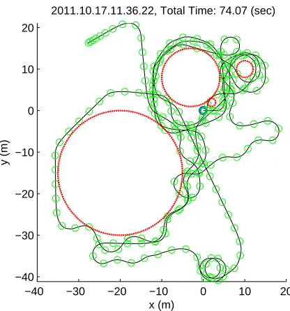
−40 −30 −20 −10 0 10 20
2011.10.17.11.36.22, Total Time: 74.07 (sec)
x (m)
y (m)
Brief Overview of Existing Literature
TheToy Problemwould be a typical target tracking with noisy measurements problem, but the presence of
obstacles makes it relatively unique.
Target tracking problems are often modeled as “hybrid systems” [1] in which the target’s state is continuous,
but the target moves according to only one of a finite number of modes or models at any time. This modeling
is applicable to theToy Problem. A very popular algorithm to solve this hybrid estimation problem is the
Interacting Multiple Models (IMM) algorithm which runs several Kalman filters [2] in parallel and merges
their results depending on measurements. The IMM algorithm is popular because it is very cost-efficient [3–5],
meaning it performs relatively well and is computationally inexpensive to calculate.
An application of the IMM algorithm is demonstrated in [6] in which a vehicle is driving along a highway.
Two conditions are of interest – maintaining a lane or changing lanes. There is a motion model and associated
“directional” process noise that corresponds to maintaining a lane, and there is a different motion model with
a different type of process noise associated with the lane change maneuver. [6] shows that the IMM algorithm
tracks the vehicle well under both conditions and quickly determines when lane changes happen. A complex
behavior is captured neatly by two models.
The Toy Problemis a simple problem that is well suited to the normal IMM algorithm – with some
assumptions on the behavior of the target, the system can be modeled using only five modes of operation.
(Refer toExperiment and Results.) However, problems often require many more modes of operation to
characterize a target’s range of motion. The IMM algorithm’s performance suffers when there are too many
motion models that overlap and compete [7]. As a result, researchers developed variable-structure multiple
model (VSMM) algorithms that perform better than the normal, fixed-structure IMM algorithm [7–11].
While the Toy Problemis not a very complicated problem that requires variable-structure algorithms,
those algorithms are of interest in this problem because of the fact that the set of models can be adapted
based on the target’s current state. For example, [7] describes a problem in which the acceleration of the
target cannot change rapidly. An overarching set of models is designed to cover all of the possible target
current acceleration. As the target’s acceleration changes, the VSMM algorithm chooses different sets of
models accordingly.
Some researchers have implemented VSMM algorithms with model selection or switching rules that are
based not only on the target’s internal state but also on the properties of the world around the target. For
example, [12] and [13] limit the available modes of operation based on the presence of roads and whether or
not the target is on a road. [12] describes a general ground target tracking problem where a target might be
navigating in an unconstrained environment (off-road), it might be near a road, or it might be constrained
to be on a piece-wise linear road. Furthermore, roads might have junctions, in which case the target can
choose from different branches. Each condition, including motion at a junction, is captured by a different set
of models, and there is a very intricate method of selecting which models are applicable. [13] expands the
on-road condition and describes how to incorporate the actual curvature of road segments as constraints.
In existing VSMM methods, the state-dependent information is captured by the strategic selection and
omission of models. The work in this thesis, in [14, 15], and in [16] consider how to embed state-dependent
information even deeper into the IMM algorithm. These methods could complement the VSMM methods
and would operate after the set of models is selected. All of these methods modify the modes’ transition
probability matrix and the modes’ likelihoods based on the target’s state.
[16] considers a problem in which a target can choose to stop randomly as an evasive maneuver. The
authors make the argument that real world targets cannot instantaneously cease their motion, and thus
the probability that the target will stop is small when its speed is large. The transition probability matrix
governing the switching of motion models depends on the speed of the target.
Guard conditions [14, 15] use a transition probability matrix that depends on the proximity to a waypoint.
An example is given in [14] where an airplane should turn toward a new destination when it arrives at a
waypoint. There are two guard conditions to model this desired behavior. The first is to switch from constant
velocity to coordinated turn when the plane’s position is near the waypoint. The second is to switch away
The work in this thesis is most similar to [14]. A very large difference is that their work is derived
theoretically when the guard conditions are of specific forms. The method described here does not have
theoretical support but is instead slightly more flexible.
Brief Overview of Proposed Methods
There are two locations in the IMM algorithm that allow the world information to be incorporated. The first
is in the model probabilities (MPs) update/remix step that uses the likelihoods of each mode. The second
is in the transition probability matrix (TPM) that tells the probability of transitioning from one mode of
operation to another mode of operation.
Just before the end of one cycle of the IMM algorithm there is one estimated state for each of the models
in the algorithm. Each of these states is assigned a value, and the values then modify the weights of their
respective models during the final update/remix step of the algorithm. This process is described in SD
Model Probabilities. Those same estimated states will interact in the mixing step to obtain the next
cycle’s initialization. Before that happens, each estimated state is propagated by all of the modes of motion
to determine “what-if” predicted states. The number of these predicted states is equal to the number of
elements in the transition probability matrix. The assigned values of these predicted states characterize the
values of the transitions, and thus they are used to modify the transition probability matrix, as described in
SD Transition Probabilities.
The value assignment is problem specific and up to the designer in the same way as the choice of models.
The section titledA State’s Value shows how value assignment is defined in this thesis. Value assignment
has an effect that is similar to penalty functions in constrained optimization problems – that is, it can convert
a tracking problem with constraints into an unconstrained one.
The layout of this thesis follows the order of building blocks. First, the Kalman filter is described, followed
by the IMM algorithm which is based on the Kalman filter. Then comes state-dependent value assignment,
the main novelty of this thesis, which modifies parts of the IMM algorithm. Finally the experiment that
implements the original problem and tests the performance of the value system is followed by an analysis and
Kalman Filter
Algorithm
Consider the following dynamics and measurement model. xk is the state of the system at timek. Ak is the
dynamics matrix that advances the state from timekto timek+ 1. wk∼ N(0, Qk) is the process noise. zk
is the measurement at timek. Hk is the sensing matrix. vk∼ N(0, Rk) is the sensor noise.
xk+1=Akxk+wk (1)
zk+1=Hk+1xk+1+vk+1 (2)
Beginning with a state estimate at time k, the Kalman filter first predicts the state at timek+ 1 then
updates the prediction when the measurement at timek+ 1 arrives. The result is an estimate of the state at
timek+ 1.
Given : ˆxk|k,Pˆk|k, Ak, Qk
ˆ
xk+1|k =Akxˆk|k (3)
ˆ
Pk+1|k =AkPˆk|kA0k+Qk (4)
The variables in Equations (3) and (4) with time index k+ 1|k are predictions. When thek+ 1th
measurement arrives, the Kalman filter first computes the filter gainKk+1.
Given : ˆxk+1|k,Pˆk+1|k, zk+1, Hk+1, Rk+1
yk+1=zk+1−Hk+1xˆk+1|k (5)
Sk+1=Hk+1Pˆk+1|kHk0+1+Rk+1 (6)
Kk+1= ˆPk+1|kHk0+1Sk−+11 (7)
After the filter gain has been computed, the Kalman filter updates the state and uncertainty estimates.
ˆ
xk+1|k+1= ˆxk+1|k+Kk+1yk+1 (8)
ˆ
Pk+1|k+1= ˆPk+1|k−Kk+1Sk+1Kk0+1 (9)
The final result of the Kalman filter is the state estimate ˆxk+1|k+1along with an estimate of its uncertainty
ˆ
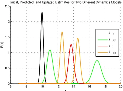
Small Visual Example
Figure 5 shows one step of the Kalman filter. Figure 6 shows one step of the Kalman filter for two different
dynamics models.
The state variable contains two quantities: a linear displacementxand a linear velocity ˙x. The measurement
z contains only displacement information; it does not directly measure the velocity. The velocity part of the
state is not shown in the two figures so that both the state and the measurement can be displayed in the
same space.
Figure 5 shows a black line that has its peak centered at ˆx0. The width of the curve is a measure of the
uncertainty of the initialization, ˆP0. The dynamics modelA0 helps to predict the state, ˆx1|0, and uncertainty,
ˆ
P1|0, at the next time step. This pair is depicted by the green curve.
A new measurement,z1, arrives at timek= 1. The measurement has a noise level, and thus the value and
uncertainty of the measurement are shown as a (red) curve instead of a single point. The actual value of the
measurement is the center of the curve. Note that there is a disparity between the green curve, the predicted
state, and the red curve, the current measurement. The Kalman filter’s role is to weigh and appropriately
combine the two.
The uncertainties of the predicted state and the measurement are weighed against each other in order to
obtain the filter’s gain. The gain is a measure of how much “correction” the predicted state requires now
that the newest measurement has arrived. The updated state, ˆx1|1, has been “corrected” by the filter and is
shown as the orange curve. Just like the other variables, this state has its value at the center of the curve,
and the width of the curve is a measure of its uncertainty.
Part of Figure 6 contains the same content as Figure 5. The other part is a repeat of the previous example,
except the dynamics matrixA0is different. For the same measurement, there are two different updated state
6 8 10 12 14 16 18 20 0
0.5 1 1.5 2 2.5
x
P(x)
Initial, Predicted, and Updated Estimates
ˆ
x0
ˆ
x1|0
z1
ˆ
x1|1
Figure 5: One step of the Kalman filtering algorithm. The initial estimate is ˆx0, and its
uncertainty ˆP0 is depicted by the Gaussian curve
centered at ˆx0 (shown in black). The green curve
is ˆx1|0, the filter’s prediction of the next state.
The red curve is the measurementz1. The orange
curve is the updated estimate ˆx1|1.
6 8 10 12 14 16 18 20
0 0.5 1 1.5 2 2.5
x
P(x)
Initial, Predicted, and Updated Estimates for Two Different Dynamics Models
ˆ
x0
ˆ
x1|0
z1
ˆ
x1|1
Figure 6: One step of the Kalman filtering algorithm, but showing two different dynamics models. The colors are the same as in Figure 5. There is only one measurementz1, but since there
are two dynamics models, there are two sets of ˆ
x1|0 and ˆx1|1. Both models are initialized at the
Interacting Multiple Models
The Interacting Multiple Models (IMM) algorithm runs several Kalman filters in parallel. The individual
filters are initialized using a mixture of results from the previous step’s filters. The output of the IMM
algorithm, the overall state estimate, is also a mixture of the individual filters’ estimates.
The IMM algorithm requires three items. The first is a set of Kalman filters, one for each ofM models or
modes of operation. The second is a probability vector,µk, that contains the set of probabilities that theith
model is in effect at the current time step,k. The third is a transition probability matrix (TPM) that tells
how probable it is to jump from modeliat time kto modelj at timek+ 1.
The IMM algorithm itself consists of three main steps.
1. Mix the model probabilitiesµi,k based on the TPM, and initialize several ˆx0j,k+1, ˆPj,k0 +1 based on the
mixed probabilities.
2. RunM separate Kalman filters starting on each ˆx0
j,k+1, ˆPj,k0 +1to obtain ˆxj,k+1, ˆPj,k+1.
3. Mix the estimates ˆxj,k+1, ˆPj,k+1 based on the model probabilities and the likelihoods of obtaining the
innovationsyj,k+1.
Step 1, Mix
For this step, the IMM algorithm requires three sets of components. It requires a vector of model probabilities
at the current timek. In addition, it requires a transition probability matrix for the current time. Finally, it
requires theM individual filters’ estimates at timek. All of these are required in order to begin the IMM
algorithm for timek+ 1. Note that this mixing step occurs beforezk+1 has arrived.
Let the column vectorµkdenote the probabilities of theM models such that theith entry is the probability
that modeliis in effect at timek. Then, let Tk be the TPM that tells the probabilities of transitioning from
modelito modelj at timek. The elements of the TPM areTji,k=P(mj,k+1|mi,k). Note that each column
ofTk must sum to one, and that
where µpk+1 is the vector of predicted mode probabilities at timek+ 1 given onlyTk and µk.
The mixing step begins by calculating the probabilitiesµij,k=P(mi,k|mj,k+1).
µij,k=Tji,kµi,k/µ p
j,k+1 (11)
Eachµij,k is the probability that mode iwas in operation at time kgiven that mode j is in operation at
timek+ 1. Note thatzk+1 has not yet arrived, soµpk+1 is a prediction.
The next part of this mixing step is to createM initializations for the individual Kalman filters. From the
previous iteration, theith Kalman filter had a state estimate ˆxi,k|k and uncertainty estimate ˆPi,k|k. These
estimates are mixed together to form new ˆx0
j,k+1 and ˆPj,k0 +1.
ˆ
x0
j,k+1=
M X
i=1
ˆ
xi,k|kµij,k (12)
ˆ
Pj,k0 +1=
M X
i=1
ˆ
Pi,k|kµij,k+Xj,k (13)
The term after the second summation isXj,k, the so called “spread of the means” [5]. Define dij,k and use it
to computeXj,k.
dij,k= ˆx0i,k+1−xˆ0j,k+1
Xj,k= M X
i=1
dij,kd0ij,kµij,k
The final results of this mixing step are the filter initializations ˆx0
j,k+1, ˆPj,k0 +1 and the predicted model
probabilitiesµpk+1. The sets ofµij,k andXj,k are not used outside of this first mixing step.
Step 2, Run Individual Filters
The first step of the IMM algorithm resulted in ˆx0
j,k+1 and ˆPj,k0 +1. This step combines those quantities with
zk+1 to obtain ˆxj,k+1 and ˆPj,k+1. This step also producesλj,k+1, the likelihood of the measurementzk+1
given thejth model is in effect. These likelihoods will be combined withµpk+1 in the next step of the IMM
algorithm to find updated model probabilitiesµk+1.
Each of the M models has its own dynamics and measurement equations similar to Equations (1) and (2).
to time dependencies. However, the same measurementzk+1 is used by allM models. Equations (14) and
(15) show the dynamics and measurement equations from the point of view of thejth model.
xj,k+1 =Aj,kxj,k+wk (14)
zk+1 =Hj,k+1xj,k+1+vk+1 (15)
The process noise is wk ∼ N(0, Qj,k). The measurement noise isvk+1∼ N(0, Rj,k+1).
This second step of the IMM algorithm is to apply the M Kalman filters. Each filter uses the same
measurement, but each filter begins at a unique ˆx0
j,k+1 and ˆPj,k0 +1. The Kalman filter algorithm is detailed in
Equations (3) to (9). Equations (3) and (4) are replaced by the following equations.
ˆ
xj,k+1|k=Aj,kxˆ0j,k+1 (16)
ˆ
Pj,k+1|k=Aj,kPˆj,k0 +1A0j,k+Qj,k (17)
The remainder continues as normal with the modification that every variable (except forzk+1) has a modelj
dependence. That is, the algorithm uses or calculates the following values.
ˆ
xj,k+1|k,Pˆj,k+1|k
zk+1, Hj,k+1, Rj,k+1
yj,k+1, Sj,k+1
Kj,k+1
ˆ
xj,k+1|k+1
ˆ
Pj,k+1|k+1
As soon asyj,k+1 andSj,k+1 are obtained, the IMM algorithm calculates the likelihood ofyj,k+1 using
the covariance matrixSj,k+1. The likelihood is calledλj,k+1.
λj,k+1=N(yj,k+1 |0, Sj,k+1) (18)
= p 1
det 2πSj,k+1
exp
−1
2y
0
j,k+1Sj,k−1+1yj,k+1
The combination of the updated state and uncertainty estimates, ˆxj,k+1|k+1 and ˆPj,k+1|k+1, with the
Step 3, Remix
The third and final step of the IMM algorithm combines the predicted mode probabilities µpk+1, the
measurement likelihoodsλj,k+1, and the individual state estimates ˆxj,k+1|k+1 and ˆPj,k+1|k+1.
The updated mode probabilities areµk+1and take into account all of the models’ likelihoods. The jth
element ofµk+1 isµj,k+1.
µj,k+1=
µpj,k+1λj,k+1
PM
i=1µ
p
i,k+1λi,k+1
(19)
The denominator of Equation (19) is a normalizing factor and is the same for allj.
The overall state estimate given by the IMM algorithm is a weighted combination of the individual filters’
estimates. The final state and uncertainty estimates ˆxk+1|k+1 and ˆPk+1|k+1 do not have model dependencies.
ˆ
xk+1|k+1=
M X
j=1
µj,k+1xˆj,k+1|k+1 (20)
ˆ
Pk+1|k+1=
M X
j=1
µj,k+1Pˆj,k+1|k+1+Xk+1 (21)
The term after the second summation is another “spread of the means.” As before in Equation (13), define
dj,k+1 and use it to calculateXk+1.
dj,k+1= ˆxk+1|k+1−xˆj,k+1|k+1
Xk+1=
M X
j=1
dj,k+1d0j,k+1µj,k+1
Prediction
The IMM algorithm can be used to obtain state and uncertainty predictions ˆxk+1|k and ˆPk+1|k. The
previously-described second and third steps of the IMM algorithm are modified slightly in order to obtain
those predictions.
The first step of the algorithm, mixing, obtains µP
k+1 along with ˆx0j,k+1 and ˆPj,k0 +1. The second step
begins as normal so that Equations (16) and (17) give individual filter predictions ˆxj,k+1|k and ˆPj,k+1|k. The
The main difference in the third step is that all λj,k+1 = 1 are equal. Therefore, µj,k+1 =µPj,k+1 in
Equations (19) to (21). The variable ˆxj,k+1|k+1is replaced by ˆxj,k+1|k and ˆPj,k+1|k+1 is replaced by ˆPj,k+1|k
inside Equations (20) and (21). Instead of obtaining ˆxk+1|k+1 and ˆPk+1|k+1, the result is ˆxk+1|k and ˆPk+1|k.
The result of the three steps, after all modifications have been made, is ˆxk+1|k and ˆPk+1|k. These two are
the IMM algorithm’s one-step prediction.
Small Visual Example
Consider a simple problem that uses an IMM filter withM = 5 models. Suppose that initially all models’
probabilities are equal.
µj,0= 1/M
Suppose also that the transition probability matrix is constant over time and tends to favor remaining in the
current mode. That is, the diagonal elements of the TPM are much larger than the off-diagonal elements.
The initial state is ˆx0, shown in Equation (22). ˆP0 is very small to indicate that the initialization is
accurate. Figure 7 shows the beginning of this example.
ˆ
x0= [10 (m),10 (m),0 (m/s),10 (m/s)]0 (22)
The five green circles of Figure 7 show the endpoints of the five models’ trajectories. These endpoints are
the position parts of the individual models’ predicted state estimates ˆxj,1|0.
The red circle is the measurementz1. The blue crosses represent the individual filters’ updated state
estimates ˆxj,1|1. Note that each of the crosses is on a line that connects a green circle ˆxj,1|0 to the red circle
z1.
The blue circle is the IMM algorithm’s final state estimate ˆx1|1. It is a linear combination of the individual
filters’ estimates. Because all of the model probabilities are equal initially, the only factor that controls
the mixing weights is the likelihood of each model given the measurement. The measurement fits the two
left-turn models much better than the straight or right-turn models. Between the two left-turn models, the
measurement is more likely to have come from the shallower turn. Thus, the blue circle is closest to the
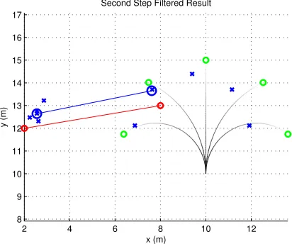
Figure 8 shows the continuation of the example. Another measurement,z2, is shown as a red circle. It is
connected to the measurementz1 using a thin red line. There are five blue crosses (two of them are almost
stacked) that correspond to the five individual filters’ updated state estimates ˆxj,2|2. The blue circle near the
new measurement is the IMM algorithm’s updated state estimate ˆx2|2. This new state estimate is connected
to the previous step’s estimate using a thin blue line.
Figure 9 shows a one-step prediction using the IMM algorithm. The example continues from before, and
now there is no new measurementz3. The blue crosses, which now represent the individual models’ predicted
states ˆxj,3|2, fan out and are not reined in by a measurement. The blue square shows the IMM algorithm’s
predicted state ˆx3|2. It is connected to the previous state estimate using a dashed blue line.
Note that the predicted state is very close to the shallow-left-turn model’s estimate. This is because of
the TPM which favors the continuation of the motion. In going from timek= 1 to k= 2, the IMM algorithm
estimated that the target performed a shallow-left-turn, and thus the algorithm predicts that the same turn
7 8 9 10 11 12 13 10
10.5 11 11.5 12 12.5 13 13.5 14 14.5 15
First Step Filtered Result
x (m)
y (m)
Figure 7: A first step using the IMM algorithm.
2 4 6 8 10 12
8 9 10 11 12 13 14 15 16 17
Second Step Filtered Result
x (m)
y (m)
Figure 8: A second step using the IMM algorithm.
−2 0 2 4 6 8 10 12
6 8 10 12 14 16
Third Step Predicted
x (m)
y (m)
State-Dependent Value Assignment
To every possible state that the target can take needs to be assigned a penalty or benefit value. In our Toy
Problem, for example, we could define a simple mapping such that every location inside of an obstacle is
assigned a zero and every other location is assigned a one. The state-to-value mapping will be used to modify
Equation (19) inSD Model Probabilitiesand Equations (10) and (11) inSD Transition Probabilities.
A State’s Value
The state-to-value mapping described in this section is only one of many possible mappings for our very
specific toy problem. Every problem will have many mappings, and the design of the state-to-value mapping
is something that must be carefully considered.
In our toy problem, there are two factors that give hints towards the design of a state-to-value mapping.
The first is that the obstacles are circles with known radii. The second is that in the toy world, a player is
“allowed” to drive the vehicle inside an obstacle, but such a maneuver is discouraged. (See Figure 2.) These
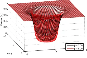
two factors can be handled by a sigmoid function, as shown in Equation (23).
Assume there are N circular obstacles, each with radius ri and with center (xi, yi), where i ∈ [1..N].
Then, consider only the position part, (x, y), of a state x. The distance between the state xand theith
obstacle isdi(x).
di(x) =p(x−xi)2+ (y−yi)2
Ifdi(x)> ri, then the statexis outside of the ith obstacle.
Define the functions(x, i) as follows.
s(x, i) = 1 1 + exp
−β(di(x)−ri)
(23)
The functions(x, i) has a sigmoidal shape. A state that is outside of theith obstacle will havedi> ri and
s(x, i) will be approximately one. A state that is inside the ith obstacle will havedi< ri ands(x, i) will be
approximately zero. The parameterβ controls the steepness of the transition between the outside region and
away from the center of an obstacle. Figure 10 shows the values of all states (x, y) with respect to an obstacle
centered at (xi, yi) = (0,0) with radiusri= 2.
The function s(x, i) is the value of the statexwith respect to the single obstaclei. In order to find the
overall value of the statexwith respect to the world, defines(x) as the minimum of allN of the functions
s(x, i).
s(x) = min
i s(x, i) (24)
SD Model Probabilities
The function s(x) gives the value of every statex. This information can be incorporated into the model
probabilities’ update step, Equation (19), with the assumption that an intelligent target will want to maneuver
toward high-valued states.
The IMM algorithm hasM modes, each of which runs a separate Kalman filter. Suppose thejth mode’s
state estimate at timek+ 1 is ˆxj,k+1. The IMM algorithm would calculate the mode probabilities and then
mix together theM estimates weighted by those probabilities in order to obtain an overall state estimate.
The procedure does not change when the states’ value information is incorporated. However, the mode
probabilities are updated as follows.
µ∗j,k+1=
µpj,k+1λj,k+1sj,k+1
PM
i=1µ
p
i,k+1λi,k+1si,k+1
(25)
For notational convenience, letsj,k+1=s(ˆxj,k+1).
−5 0
5 −5
0
5 0 0.2 0.4 0.6 0.8 1
Value Function Using β = 3.00 and 6.00 for a Single Obstacle
x (m) y (m)
Value of (x,y)
β = 3.00
β = 6.00
SD Transition Probabilities
The functions(x) gives a value to every statex. The states’ value information can be embedded into the
transition probability matrix under the assumption that an intelligent target will want to maneuver toward
high-valued states.
The first step of each iteration of the IMM algorithm is a mixing step in which mode probabilities are
predicted based on the system’s transition probability matrix. At the end of the previous step, the IMM
algorithm hadM state estimates ˆxi,k|k that were updated by using the measurementzk. To incorporate the
world information, the the IMM algorithm will use the transition probability matrixT∗
k to predict the model
probabilities at timek+ 1, whereT∗
k is a modification of the originalTk shown in Equation (10).
The mixing step in the IMM algorithm mixes together mode estimates. It considers the possibility that
modeiwas in effect previously when modej is in effect currently. Embedding the states’ value information
into the transition probability matrix relies on those “what-if” state estimates. Define the state ˆxj,k+1|i,k as
follows.
ˆ
xj,k+1|i,k=Aj,kxˆi,k|k (26)
The state ˆxj,k+1|i,k is a prediction of the state of the target that would arise if modeiwere in effect at time
kbut modej is used to propagate the state to timek+ 1.
There are M2states ˆx
j,k+1|i,k, one for each possible transition. The value of each state issji,k.
sji,k=s(ˆxj,k+1|i,k) (27)
These states’ values are merged together with the original transition probability matrixTk to obtainTk∗. Tk
is the matrix of elements [Tji,k]. Suppose that [sji,k] is a matrix that contains all of the values ofsji,k.
Tk∗= col norm [sji,k].∗ [Tji,k]
(28)
The “dot-star” .∗ operation means element by element multiplication and in this case results in a matrix.
Each of the transition probability matrix’scolumnsmust sum to one, thus the col norm function is applied
to the resulting matrix.
The matrix T∗
k is obtained before Equations (10) and (11). Those two equations are modified to useTk∗
Small Visual Example
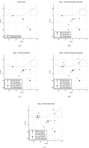
Figure 11 is a small visual example that shows a change in the estimated state due to the presence of an
obstacle. Figure 11a shows the initial location and orientation of the target, specified by theblue circle
andblue dot, as well as the first two measurements that will arrive, shown as red circles. There is no
ground truth for this case, as the purpose of this example is not to track the target. Actual tracking will be
examined in more detail inExperiment and Results.
Figure 11b shows five individual modes’ estimates after the first measurement has arrived. The blue
squarescorrespond to the normal IMM algorithm’s estimates while thegreen X’scorrespond to SD TPM,
the IMM algorithm with world information incorporated into the transition probability matrix. The normal
TPM is fixed and has large diagonal elements, while the SD TPM modifies the normal TPM at every time
step. The initial location of the target and the first measurement are not close to any obstacles, and thus the
normal and SD TPM modes’ estimates match exactly. Figure 11c shows that the overall normal and SD
TPM state estimates also coincide. The normal estimate is shown as a heavy blue square, and the SD
TPM estimate is shown as aheavy green X.
Figure 11d takes place during the second time step. The blue squares and green X’s have the same
meaning as before, except now they are calculated using the second measurement. Notice that the normal
estimates and the SD TPM estimates are different now due to the proximity of an obstacle. Figure 11e shows
the overall normal estimate as a heavy blue square and the overall SD TPM estimate as a heavy green X.
The SD TPM estimate lies just outside the obstacle.
The measurement noise is assumed to be relatively small in this example, and thus the IMM algorithm’s
estimates hug the measurements. Incorporating the world information makes a difference despite the small
−5 −3 −1 1 3 −5
−3 −1 1 3
x (m)
y (m)
Initial Layout
Measurements
(a)
−5 −3 −1 1 3
−5 −3 −1 1 3
x (m)
y (m)
Step 1, Individual Modes’ Estimates
Measurements Normal Modes SD TPM Modes
(b)
−5 −3 −1 1 3
−5 −3 −1 1 3
x (m)
y (m)
Step 1, Filtered Estimates
Measurements Normal Modes SD TPM Modes Normal Filtered SD TPM Filtered
(c)
−5 −3 −1 1 3
−5 −3 −1 1 3
x (m)
y (m)
Step 2, Individual Modes’ Estimates
Measurements Normal Modes SD TPM Modes Normal Filtered SD TPM Filtered
(d)
−5 −3 −1 1 3
−5 −3 −1 1 3
x (m)
y (m)
Step 2, Filtered Estimates
Measurements Normal Modes SD TPM Modes Normal Filtered SD TPM Filtered
(e)
Experiment and Results
The section titledToy Problem describes how ground truth trajectories are created. Samples come from
the position part of the ground truth every T = 0.35 seconds, and these samples are used as the basis
of the tracking experiment. The purpose of the experiment is to compare the performance of the IMM
algorithm under the normal case with no state-dependent features to the IMM algorithm with state-dependent
modifications.
Experimental Design
The first step of designing the experiment is to design the IMM algorithm’s model set. This model set should
capture the possible maneuvers that the target can take while simultaneously being as simple as possible. In
order to simplify the design, we chose sections of ground truth in which the speed of the target is constant,
thus avoiding the need to model linear accelerations. This simplification would be an acceptable assumption
in a real game, because generally a skilled player would maneuver without slowing down in order to gain the
maximum number of points.
We chose to track the position and the velocity of the target. The state variable isx. The variablesx
andy represent coordinates.
x= [x, y,x,˙ y˙]0 (29)
The model set that we chose consists of five constant turn models with varying turn rates. Two left-turn
models haveω1 = 1.42×2π rad/s andω2= 0.71×2πrad/s. Two right-turn models haveω4=−ω2 and
ω5=−ω1. A final model hasω3= 0, which corresponds to going straight. The dynamics matrix of a constant
turn model, adapted from [5], is as follows.
A(ω, T) =
1 0 sin(ωT)
ω
cos(ωT)−1
ω
0 1 1−cos(ωT)
ω
sin(ωT)
ω
0 0 cos(ωT) −sin(ωT)
0 0 sin(ωT) cos(ωT)
Figure 12 shows the possible combinations of the five models after two time steps. The green circles
represent the end position, and each black line shows the trajectory that the target would have taken to get
to an endpoint. Even though the mode sequences [ω2, ω2] and [ω1, ω5] have the same endpoint, the resulting
orientations are different.
The second step of the design of the experiment is to design various filters. We implemented and tested
four variations of the IMM algorithm, all of which use the same model set. The first two variations have a
constant transition probability matrix with large diagonal elements. The first variation is the standard IMM
algorithm with no state-dependent features. This case is called “Normal.” The second algorithm is the IMM
algorithm with the world information embedded into the model probabilities, as described in the sectionSD
Model Probabilities. This case is called “SD MPs.”
The third and fourth variations have a new transition probability matrix at every time step. The third
algorithm is the IMM algorithm with the world information embedded into the transition probability matrix,
as described in the section SD Transition Probabilities. This case is called “SD TPM.” The fourth
variation is the IMM algorithm with world information embedded into both the model probabilities and the
transition probability matrix. This case is called “SD Both.”
All three of the state-dependent variations use the value functions(x) described in Equation (24). The
functions(x) knows the locations and sizes of the obstacles in the toy world.
5 10 15
9 10 11 12 13 14 15 16 17 18
Possible Two−Step Trajectories When Using 5 Modes of Motion
x (m)
y (m)
Figure 12: Possible sequences over two time steps. The initial state is [x, y,x,˙ y˙]0= [10,10,0,10]0. Each time
The final step of the design of the experiment is to prepare true trajectory samples with corresponding
noisy measurements. Figures 18 to 29 show the snippets of true trajectories that were chosen. Each green
circle in those figures represents the truth at a particular time step. Those serve as the reference samples and
are corrupted by noise of varying degree to obtain the measurements.
The measurement model used in the IMM algorithms matches the mechanism by which the measurements
are created. The measurement model, shown in Equation (31), uses position-only measurements and has
additive Gaussian noisevk+1.
zk+1=Hk+1xk+1+vk+1 (31)
Hk+1=H =
1 0 0 0
0 1 0 0
The noise vk+1 has a parameterσz2, as shown in Equation (32).
vk+1∼ N(0, Rk+1)
Rk+1=R=
σ2
z 0
0 σ2
z
(32)
The experiment runs all of the filters for each value of σ2
z in order to see if a varying noise level affects the
filters in different ways. For example, Figure 18 has within it Figure 18a to Figure 18g, one set of results for
Results
Four variations of the IMM algorithm try to estimate and predict the motion of the target. There are several
ground truth trajectories, one for each of Figures 18 to 29.
Suppose one of the ground truth trajectories has N+ 1 true samples, samples that are not corrupted by
noise. The first sample is used as the initialization of the algorithms. (The first sample is the sample, green
circle, that is “behind” the blue circle.) The remainingN samples are corrupted by additive Gaussian noise
with a specific σ2
z.
The measurements z1tozN have corresponding true statesx1 toxN. The filters use those measurements
to obtain state estimates ˆx1|1, ˆx2|2, ..., ˆxN|N. The difference between the truth and the estimate is ˜xk|k.
˜
xk|k=xk−xˆk|k (33)
The filters also use those measurements to obtain state predictions ˆx1|0, ˆx2|1, ..., ˆxN|N−1. The difference
between the truth and the prediction is ˜xk|k−1.
˜
xk|k−1=xk−xˆk|k−1 (34)
The estimation error,ee, is defined as the average distance between the true position and the estimate of
the position.
ee= 1
N
N X
k=1
q
(Hxˆk|k)0(Hxˆk|k) (35)
The prediction error, ep, is defined as the average distance between the true position and the prediction of
the position.
ep= 1
N
N X
k=1
q
(Hxˆk|k−1)0(Hxˆk|k−1) (36)
Note that botheeandep are scalars.
There is one value of eeper trial for each of the four algorithms in the experiment, plus there is one value
ofeefor the measurements themselves for each trial. Similarly, there is one value of ep per trial for each of
the four algorithms. Conversely, there is noep for the measurements. Figures 18a to 29g show the average
The value of ¯ee that corresponds to the measurements is related to the noise levelσ2z. Since the variable
˜
xk|k is a zero-mean Gaussian random variable with covariance matrixR= diag(σz2, σz2), the magnitude of
˜
xk|k is a Rayleigh distributed random variable with meanµ= ¯ee.
µ= r
π
2σ
2
z (37)
This relationship gives a relative scale to the estimation and prediction errors.
In Figures 18a to 29g, the measurements’ estimation error is always bolded because it is the baseline
reference, and there is at most one other value in each column that has been bolded. The other bolded value
Discussion
Figures 18a to 29g show the results of the experiment described inExperiment and Results. There are
twelveground truth cases, each of which contains cases forseven different measurement noise levels. Thus,
the experiment contains a total ofeighty-fourparameter combinations. One purpose of this section is to try
to identify patterns in the results, and to that end two major questions need to be addressed.
1. Does knowledge of the environment actually make a difference in tracking performance?
2. Is there a difference between implementing the world information in the model probabilities as opposed to
the transition probability matrix?
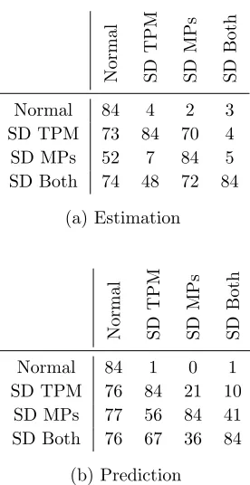
Figure 13 provides some counts that might help to answer those questions.
Normal SD
TPM
SD
MPs
SD
Both
Normal 84 4 2 3
SD TPM 73 84 70 4
SD MPs 52 7 84 5
SD Both 74 48 72 84
(a) Estimation
Normal SD
TPM
SD
MPs
SD
Both
Normal 84 1 0 1
SD TPM 76 84 21 10
SD MPs 77 56 84 41
SD Both 76 67 36 84
(b) Prediction
State-Dependent Performance
The experiment contains four variations of the IMM algorithm. In addition to calling them “Normal,” “SD
TPM,” “SD MPs,” and “SD Both,” we can refer to them as the first, second, third, or fourth algorithm,
respectively. This is the order in which the algorithms were implemented as well as the order in which the
results are displayed. Figure 13 counts how many times algorithmiwas better than algorithmj over the
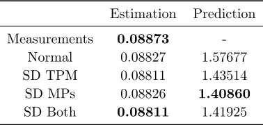
eighty-fourcases. Consider Figure 18a, reproduced here for convenience.
Estimation Prediction
Measurements 0.08873
-Normal 0.08827 1.57677
SD TPM 0.08811 1.43514
SD MPs 0.08826 1.40860
SD Both 0.08811 1.41925
The Estimation column shows the values of ¯ee,i, and the Prediction column shows the values of ¯ep,ifor
the case of 18a. (Add an algorithm subscript ito Equations (35) and (36).) For every pair i, j ∈[1..4]2,
add one to thei, jth entry of Figure 13a if ¯ee,i is less than ¯ee,j. Also add one to thei, jth entry ifiis equal
toj. Note that ¯ee,i is never less than itself. This process is performed over all eighty-four cases to obtain
Figure 13a. The process is repeated again using ¯ep,i to obtain Figure 13b.
Figure 13 shows that the three state-dependent variations of the IMM algorithm very frequently perform
better, on average, than the “Normal” algorithm both for estimation and for prediction. This can be seen in
two ways. In the first column of Figures 13a and 13b, the entries that correspond to the state-dependent
algorithms are very high, with the exception of “SD MPs” in the Estimation case, meaning that the
state-dependent variations frequently perform better than the “Normal” case. A similar conclusion comes from the
first row of each of the two figures; the “Normal” case is almost never better than the state-dependent cases.
In Estimation, “SD MPs” is better than “Normal” 52 times, “Normal” is better than “SD MPs” 2 times, and
the remaining 30 times the two were equal (within five decimal places). Seven of the equivalent performances
come from Figure 25 because there are no obstacles.
It is important to note that Figure 13 does not give an indication of how much better the state-dependent
algorithms performed. It merely counts how many times the state-dependent algorithms performed better by
place. When the measurement noiseσ2
z is very low, there is not much room for improvement. Even in 18g,
the highestσ2
z of Figure 18, the estimation performance of the state-dependent algorithms is not much better
than that of the “Normal” algorithm.
Examining the actual numbers in Figures 18a to 29g shows that the state-dependent predictors perform
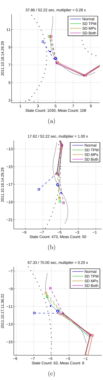
better than the “Normal” predictor by a qualitatively discernible amount. Further evidence is given by
Figure 14 and Figure 15 in which the state-dependent algorithms predict correctly that the target will
maneuver to avoid the obstacles.
State-Dependent Comparison
According to Figure 13a and Figure 13b, there are differences between using “SD MPs,” “SD TPM,” and
“SD Both.” The effects of the differences can be seen by carefully examining Figure 13, but the causes of the
differences are not clear yet. The relative differences between the variations depend as much on the choice of
the state-to-value mapping as they do on the methods of incorporating that information.
Figure 13a shows that “SD TPM” performs better than “SD MPs” a majority of the time in estimation.
Further, it shows that “SD Both” is at least as good as, if not better than, “SD TPM” in the majority of
cases. Conversely, Figure 13b shows that “SD MPs” often predicts better than “SD TPM.” It also shows
that “SD MPs” is roughly equivalent in performance to “SD Both.” The combination algorithm, “SD Both,”
can take both the good parts and the bad parts of the individual variations “SD TPM” and “SD MPs,” thus
the challenge becomes to differentiate between “SD TPM” and “SD MPs.”
It seems that “SD TPM” is not as good as “SD MPs” for prediction, but it is better for estimation.
Generally, the IMM algorithm at the k+ 1th time step has the ability to lessen the strength of thekth
measurement because of the mixing step, as shown in Equations (11) to (13). The “SD TPM” algorithm
has even more of that power because of the fact that the transition probability matrix can be very heavily
modified, as in Equation (28), before the mixing step takes place. I believe this causes the predictions of
the “SD TPM” algorithm to be more wild than the predictions of the “SD MPs” algorithm, evidenced by
Figure 16 and Figure 17. Even though the predictions of “SD TPM” are wild, they appear to be good mixing
−11 −9 −7 −5 −3 −9
−7 −5 −3 −1
52.93 / 74.15 sec, multiplier = 0.42 x
State Count: 1397, Meas Count: 151
2011.10.17.11.36.22
(a) Window of ground truth around k= 151.
−11 −9 −7 −5 −3 −9
−7 −5 −3 −1
52.93 / 74.15 sec, multiplier = 0.42 x
State Count: 1397, Meas Count: 151
2011.10.17.11.36.22
Normal SD TPM SD MPs SD Both
(b) Four predicted states ˆx152|151.
−13 −11 −9 −7 −5 −7
−5 −3 −1 1
53.31 / 74.15 sec, multiplier = 0.42 x
State Count: 1408, Meas Count: 152
2011.10.17.11.36.22
Normal SD TPM SD MPs SD Both
(c) Four predicted states ˆx153|152.
Figure 14: Truth and Predictions.
1 3 5 7 9
3 5 7 9 11
37.86 / 52.22 sec, multiplier = 0.28 x
State Count: 1030, Meas Count: 108
2011.10.18.14.29.29
Normal SD TPM SD MPs SD Both
(a)
−9 −7 −5 −3 −1 −21
−19 −17 −15 −13
17.62 / 52.22 sec, multiplier = 1.00 x
State Count: 473, Meas Count: 50
2011.10.18.14.29.29
Normal SD TPM SD MPs SD Both
(b)
−9 −7 −5 −3 −1 −15
−13 −11 −9 −7
67.33 / 70.00 sec, multiplier = 0.20 x
State Count: 63, Meas Count: 8
2011.10.17.11.36.22
Normal SD TPM SD MPs SD Both
(c)
In particular cases, the aforementioned general tendencies do not occur. In the case of Figure 19, “SD
TPM” is often better than “SD MPs” for both estimation and prediction. Alternatively, Figure 23 shows that
the best estimator depends on the noise level. It is not clear whether these differences are inherent properties
of the world information embedding methods or if they are more due to the specific choice of state-to-value
mapping.
The Value Function
There are certain valid maneuvers in this specific world that the specific choice of value function deems as
very improbable. Figure 17 is an example of a case in which the target continues to maneuver inside of an
obstacle’s boundary. It is clear that the state-dependent algorithms behave correctly according to the choice
of value function but incorrectly with respect to the actual rules governing the toy problem. This causes
large estimation and prediction errors for all of the state-dependent algorithms.
The inaccuracy of the value function also might explain why the performance rankings of the algorithms
vary so much in Figure 23. Determining whether the performance variations are due to the value function or
to the method by which the world information is incorporated requires more research.
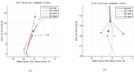
Regardless, a better value function would improve the tracking performance for this specific player in
this specific toy problem. For example, Figure 16a shows that the “SD MPs” prediction stays close to the
boundary of the obstacle while the “SD TPM” and “SD Both” predictions push away from the edge. A
slightly modified value function could give more value to the area that hugs the boundaries, because this
−13 −11 −9 −7 −5 7
9 11 13 15
4.67 / 52.22 sec, multiplier = 0.28 x
State Count: 116, Meas Count: 13
2011.10.18.14.29.29
Normal SD TPM SD MPs SD Both
(a)
−9 −7 −5 −3 −1
−19 −17 −15 −13 −11
17.31 / 52.22 sec, multiplier = 0.28 x
State Count: 465, Meas Count: 49
2011.10.18.14.29.29
Normal SD TPM SD MPs SD Both
(b)
Figure 16: The combination of the value function, the transition probability matrix, and the methods of embedding the world information sometimes allows SD MPs to perform better than SD TPM.
−5 −3 −1 1 3
3 5 7 9 11
65.81 / 103.60 sec, multiplier = 0.55 x
State Count: 1765, Meas Count: 188
2011.10.14.14.45.22
Normal SD TPM SD MPs SD Both
Conclusion
All three of the Goalshave been accomplished. The target is controlled by a human player in real time
in order to generate the ground truth trajectories for the simulations. The player generally avoids certain
obstacle regions in the world, and this world information is incorporated into the IMM algorithm. Knowledge
of the world information allows state-dependent variations of the IMM algorithm to estimate and predict the
motion of the target better than the normal version.
There are three state-dependent variations of the IMM algorithm. State-dependent model probabilities,
“SD MPs,” embeds the world information into the final remixing step of the IMM algorithm. State-dependent
transition probability matrix, “SD TPM,” incorporates the world information into the transition probability
matrix before the first mixing step of the IMM algorithm. A combination, “SD Both,” modifies both the
model probabilities and the transition probability matrix.
Based on the set of ground truth trajectories and the simulation results, “SD TPM” seems to perform
betterthan “SD MPs” for estimation butworsefor prediction. The combination, “SD Both,” often performs
at least as well as the other two. All three of the variations almost always performbetterthan the “Normal”
algorithm. The estimation performance increase is not always significant, but the prediction performance is
almost always qualitatively better.
The value function presented inA State’s Valueis relatively simple and does not accurately capture the
states’ values from the point of view of the specific player in this specific toy world. A better value function
certainly would improve the tracking performance of the state-dependent IMM algorithms. Regardless,
the simple value function is enough to improve the performances of the state-dependent algorithms when
compared to the normal algorithm.
The value function must be tailored to a specific problem, but the method of incorporating the world
information into the IMM algorithm is generally applicable. Specific performance details depend on both the
References
[1] Y. Bar-Shalom, X. R. Li, and K. C. Chang, 1990.
Nonstationary noise identification with the interacting multiple model algorithm. Proceedings of the 5th
IEEE International Symposium on Intelligent Control, vol. 1, pp. 585–589
[2] R. E. Kalman, 1960.
A new approach to linear filtering and prediction problems. Transactions of the ASME–Journal of Basic Engineering, vol. 82(Series D): pp. 35–45
[3] X. R. Li and Y. Bar-Shalom, 1992.
A recursive hybrid system approach to noise identification.First IEEE Conference on Control Applications, 1992., vol. 2, pp. 847–852
[4] X. R. Li and Y. Bar-Shalom, 1993.
Performance prediction of the interacting multiple model algorithm. IEEE Transactions on Aerospace and Electronic Systems, vol. 29(3): pp. 755–771
[5] X. R. Li and Y. Bar-Shalom, 1993.
Design of an interacting multiple model algorithm for air traffic control tracking. IEEE Transactions on
Control Systems Technology, vol. 1(3): pp. 186–194
[6] R. Toledo-Moreo and M. A. Zamora-Izquierdo, 2009.
Imm-based lane-change prediction in highways with low-cost gps/ins. IEEE Transactions on Intelligent
Transportation Systems, vol. 10(1): pp. 180–185
[7] X. R. Li and Y. Bar-Shalom, 1996.
Multiple-model estimation with variable structure. IEEE Transactions on Automatic Control, vol. 41(4): pp. 478–493
[8] X. R. Li, Y. Zhang, and X. Zhi, 1997.
Multiple-model estimation with variable structure: model-group switching algorithm. Proceedings of the
36th IEEE Conference on Decision and Control, 1997., vol. 4, pp. 3114–3119
[9] X. R. Li, X. Zwi, and Y. Zwang, 1999.
Multiple-model estimation with variable structure. iii. model-group switching algorithm. IEEE
Transactions on Aerospace and Electronic Systems, vol. 35(1): pp. 225–241
[10] X. R. Li, 2000.
Multiple-model estimation with variable structure. ii. model-set adaptation. IEEE Transactions on
Automatic Control, vol. 45(11): pp. 2047–2060
[11] X. Wang, S. Challa, R. Evans, and X. R. Li, 2003.
Minimal submodel-set algorithm for maneuvering target tracking. IEEE Transactions on Aerospace and Electronic Systems, vol. 39(4): pp. 1218–1231
[12] T. Kirubarajan, Y. Bar-Shalom, K. R. Pattipati, and I. Kadar, 2000.
Ground target tracking with variable structure imm estimator. IEEE Transactions on Aerospace and Electronic Systems, vol. 36(1): pp. 26–46
[13] M. Zhang, S. Knedlik, and O. Loffeld, 2008.
An adaptive road-constrained imm estimator for ground target tracking in gsm networks. 2008 11th
[14] I. Hwang and C. E. Seah, 2006.
An estimation algorithm for stochastic linear hybrid systems with continuous-state-dependent mode transitions. 2006 45th IEEE Conference on Decision and Control, pp. 131–136
[15] C. E. Seah and I. Hwang, 2009.
State estimation for stochastic linear hybrid systems with continuous-state-dependent transitions: An imm approach. IEEE Transactions on Aerospace and Electronic Systems, vol. 45(1): pp. 376–392
[16] S. Zhang and Y. Bar-Shalom, 2011.
Tracking move-stop-move targets with state-dependent mode transition probabilities. IEEE Transactions
on Aerospace and Electronic Systems, vol. 47(3): pp. 2037–2054
[17] D. J. Kershaw, 1999.
Issues in single target tracking with state dependent detection probability. Proceedings of IDC 99 on
Information, Decision and Control, pp. 99–104
[18] V. P. Jilkov and X. R. Li, 2004.
Online bayesian estimation of transition probabilities for markovian jump systems. IEEE Transactions on Signal Processing, vol. 52(6): pp. 1620–1630
[19] Z. Ding and H. Leung, 2008.
Evaluation of two imm-based algorithms in real radar tracking environments. 2008 Canadian Conference
on Electrical and Computer Engineering, pp. 1569–1574
[20] X. R. Li and V. P. Jilkov, 2010.
Survey of maneuvering target tracking. part ii: Motion models of ballistic and space targets. IEEE
Transactions on Aerospace and Electronic Systems, vol. 46(1): pp. 96–119
[21] Y. Liu and X. R. Li, 2011.
Sequential multiple-model detection of target maneuver termination. 2011 Proceedings of the 14th
International Conference on Information Fusion (FUSION), pp. 1–8
[22] D. Gruyer and E. Pollard, 2011.
Credibilistic imm likelihood updating applied to outdoor vehicle robust ego-localization.2011 Proceedings
of the 14th International Conference on Information Fusion (FUSION), pp. 1–8
[23] D. Gu, 2011.
Appendices
Simulation Results
−40 −30 −20 −10 0 10 20 30
−40 −30 −20 −10 0 10 20
2011.10.17.11.36.22, Total Time: 74.07 (sec)
x (m)
y (m)
Estimation Prediction
Measurements 0.08873
-Normal 0.08827 1.57677
SD TPM 0.08811 1.43514
SD MPs 0.08826 1.40860
SD Both 0.08811 1.41925
(a) Averages of 300 Runs,σ2
z = 0.005
Estimation Prediction
Measurements 0.12572
-Normal 0.12439 1.61050
SD TPM 0.12407 1.46384
SD MPs 0.12438 1.44233
SD Both 0.12407 1.44316
(b) Averages of 300 Runs,σ2
z= 0.010
Estimation Prediction
Measurements 0.19813
-Normal 0.19462 1.69597
SD TPM 0.19352 1.53771
SD MPs 0.19451 1.52323
SD Both 0.19347 1.51042
(c) Averages of 300 Runs,σ2z= 0.025
Estimation Prediction
Measurements 0.27937
-Normal 0.27229 1.78459
SD TPM 0.27028 1.62484
SD MPs 0.27196 1.61392
SD Both 0.27012 1.59280
(d) Averages of 300 Runs,σ2
z= 0.050
Estimation Prediction
Measurements 0.39631
-Normal 0.38525 1.93268
SD TPM 0.38058 1.77883
SD MPs 0.38448 1.76810
SD Both 0.38006 1.74156
(e) Averages of 300 Runs,σ2
z= 0.100
Estimation Prediction
Measurements 0.62607
-Normal 0.60578 2.20458
SD TPM 0.59379 2.07286
SD MPs 0.60353 2.04680
SD Both 0.59263 2.02831
(f) Averages of 300 Runs,σ2
z = 0.250
Estimation Prediction
Measurements 0.88759
-Normal 0.85571 2.51311
SD TPM 0.83711 2.39872
SD MPs 0.84918 2.34708
SD Both 0.83372 2.34748
(g) Averages of 300 Runs,σz2= 0.500
−30 −25 −20 −15 −10 −5 0 −35
−30 −25 −20 −15 −10 −5
2011.10.17.11.36.22, Total Time: 5.00 (sec)
x (m)
y (m)
Estimation Prediction
Measurements 0.08744
-Normal 0.08739 2.07265
SD TPM 0.08735 1.73294
SD MPs 0.08739 1.70343
SD Both 0.08735 1.60858
(a) Averages of 300 Runs,σ2
z = 0.005
Estimation Prediction
Measurements 0.12314
-Normal 0.12298 2.10733
SD TPM 0.12269 1.75524
SD MPs 0.12298 1.74120
SD Both 0.12269 1.63091
(b) Averages of 300 Runs,σ2
z= 0.010
Estimation Prediction
Measurements 0.19788
-Normal 0.19664 2.18962
SD TPM 0.19556 1.82160
SD MPs 0.19664 1.85959
SD Both 0.19556 1.68555
(c) Averages of 300 Runs,σ2
z= 0.025
Estimation Prediction
Measurements 0.28012
-Normal 0.27856 2.25738
SD TPM 0.27500 1.90231
SD MPs 0.27856 1.96382
SD Both 0.27500 1.76260
(d) Averages of 300 Runs,σ2
z= 0.050
Estimation Prediction
Measurements 0.39782
-Normal 0.38691 2.35647
SD TPM 0.37949 2.03984
SD MPs 0.38689 2.04847
SD Both 0.37949 1.88700
(e) Averages of 300 Runs,σ2
z= 0.100
Estimation Prediction
Measurements 0.63475
-Normal 0.60169 2.63397
SD TPM 0.58653 2.31658
SD MPs 0.59944 2.24449
SD Both 0.58583 2.13093
(f) Averages of 300 Runs,σ2
z = 0.250
Estimation Prediction
Measurements 0.87034
-Normal 0.79279 2.89796
SD TPM 0.78164 2.63250
SD MPs 0.78783 2.47478
SD Both 0.77894 2.42925
(g) Averages of 300 Runs,σ2
z = 0.500
![Figure 12: Possible sequences over two time steps. The initial state is [x, y, ˙x, ˙y]′ = [10, 10, 0, 10]′](https://thumb-us.123doks.com/thumbv2/123dok_us/8941745.1851113/30.612.205.409.489.665/figure-possible-sequences-time-steps-initial-state-x.webp)