Volume 31 - Article 21 | Pages 625–658

(1)

DEMOGRAPHIC RESEARCH

VOLUME 31, ARTICLE 21, PAGES 625

−

658 PUBLISHED 16 SEPTEMBER 2014

http://www.demographic-research.org/Volumes/Vol31/21/ DOI: 10.4054/DemRes.2014.31.21

Research Article

Local determinants of crime:

Do military bases matter?

Alfredo R. Paloyo

Colin Vance

Matthias Vorell

©2014 Alfredo R. Paloyo, Colin Vance & Matthias Vorell.

This open-access work is published under the terms of the Creative Commons Attribution NonCommercial License 2.0 Germany, which permits use, reproduction & distribution in any medium for non-commercial purposes, provided the original author(s) and source are given credit.

(2)

1 Introduction 626

2 Young men and crime 631

3 The transformation of the German armed forces 637

4 Data description 640

5 Estimation strategy and results 646

6 Conclusion 649

References 651

(3)

Local determinants of crime: Do military bases matter?

Alfredo R. Paloyo1

Colin Vance2

Matthias Vorell3

Abstract

BACKGROUND

The majority of crime is committed by young men, and young men comprise the majority of the military-base population. The confluence of these two empirical regularities invites a scientific look at the contribution of a military base to criminal activity in its geographic periphery.

OBJECTIVE

We estimate the impact on criminal activity of the massive base realignments and closures that occurred in Germany for the period 2003–2007. In particular, we examine breaking and entering, automobile-related crime, violent crime, and drug-related crime. METHODS

We use a fixed-effect model to account for time-invariant unobservable elements in a panel of 298 military bases. We also take advantage of geographic information system software to mitigate issues arising from the spatial nature of the dataset.

RESULTS

The estimates indicate that the base realignments and closures did not have a significant impact on criminal activity surrounding bases. Traditional correlates of crime remain statistically significant in our specifications.

CONCLUSIONS

Although crime is largely committed by young men, we find that the closure of military bases, which are staffed primarily by young men, does not have an impact on criminal

1_{University of Wollongong, Australia. Rheinisch-Westfälisches Institut für Wirtschaftsforschung (RWI),} Germany. Forschungsinstitut zur Zukunft der Arbeit (IZA), Germany. Corresponding Author. E-Mail: [email protected].

(4)

activity. For matters of regional policy, we find that arguments pertaining to criminal activity generated by military bases are not supported by data.

COMMENTS

Economic wellbeing, as measured by real GNP and relative disposable income, is negatively associated with crime. Higher unemployment has a positive association. Regions with higher percentage of foreigners also have higher levels of crime.

1. Introduction

Against the backdrop of the transformation of the German Federal Defense Forces, we examine the socioeconomic impact of military bases on the surrounding communities. In particular, we focus on the effects of military bases and military personnel on the level of crime in the surrounding area. The realignment of the German Federal Defense Forces gives us a unique opportunity to use a natural experiment to estimate the causal impact of military base closures on crime.

While the cost of military base closures is usually estimated in terms of its impact on regional output (see, for instance, Paloyo et al. 2010), a full accounting of the costs must include social costs, such as crime. In this paper, we attempt to capture this particular aspect of base closures. Others have also recognized the importance of estimating these indirect impacts (e.g., Thanner 2006; aus dem Moore 2012).4_{In the}

pursuit of quantifying the impact on criminal activity around the base, we also aim to document the typical covariates of crime, such as legal economic opportunities (as indicated by, say, household income and regional output), the percentage of foreigners, and the percentage of young adults.

Military service and crime have long been linked in the literature. There is ample evidence that conscription could lead men to commit crimes in the future, and Germany just recently abolished compulsory military service. For example, using a natural experiment in the assignment of draft-eligibility status through a lottery system in Argentina, Galiani, Rossi, and Schargrodsky (2011) find that participation in military service increases the likelihood of having a criminal record in the future, particularly when the crime involves weapons. Lindo and Stoecker (2014) demonstrate that “military service increases the probability of incarceration for a violent crime” although it does seem to have an opposite effect for the probability of incarceration for a nonviolent crime. Violent acts also increased for combat-exposed Vietnam veterans,

(5)

particularly for blacks (Rohlfs 2010).5_{It is therefore conceivable that military personnel}

could have an impact on the level of crime observed around the base’s surroundings. Being involved in the military can increase the likelihood of engaging in criminal activity for a variety of reasons. Psychologically, the most obvious is perhaps the exposure to extremely stressful situations, including intensive training and combat. Exposure to combat, in particular, can elicit a stress reaction ‒ combat fatigue ‒ that is widely reported to be a leading cause for post-traumatic stress disorders among soldiers and veterans. Because of the military training, access costs associated with weapons are much lower for military personnel. For instance, knowledge of operation of a pistol or rifle is immediately provided.

Moreover, soldiers are removed from their usual social environment and are expected to rapidly conform to the culture within the military as an institution. This causes an enormous amount of stress. Much of the training occurs in an exclusive environment or social milieu that is, by nature, prone to a violent response. As an isolated and insulated institution, peer effects can be expected to manifest themselves much more strongly, amplifying negative attitudes that may arise out of a masculine military environment.

The impact of military service has also been shown to be generally negative for the labor-market performance of veterans.6_{This is because of a variety of reasons,}

including the depreciation of their human capital while in service and their delayed entry in the civilian labor market. Due to this inferior economic situation, engaging in criminal activity might become an attractive alternative for this group of individuals.

Finally, at the aggregate level, the variation in the level of criminal activity can be attributed mechanically to the reduction in the pool of potential criminal offenders when a military base shuts down or reduces its personnel complement. Since personnel are typically relocated, there are simply fewer people to commit crime. The data, described below, allow us to observe this at a particular geographic level of aggregation, at the cost of not being able to identify exactly which person (military serviceman or not) committed the crime.

Crime is a complex social phenomenon that deserves special focus from social scientists. Various aspects of crime have been examined by psychologists, sociologists, lawyers, political scientists, and, beginning with the work of Becker (1968) and its extension by Ehrlich (1973), by economists as well. Applications of economic theories

5_{Siminski, Ville, and Paull (2013) are unable to demonstrate a qualitatively similar effect for Australian} soldiers, which they attribute partly to the less aggressive and realistic training that Australian conscripts received.

(6)

of rational choice tend to explain the observed trends in deviant behavior quite well.7

For example, changes in the economic milieu ‒ as can potentially happen with the closure of a military base ‒ have been shown to have an impact on criminal activity. Bushway et al. (2012) list four reasons that relate poor economic situations to crime: reduction in opportunities for legitimate economic activities, reduction in criminal opportunities (poorer people tend to be robbed less, for example), reduction in the consumption of drugs and alcohol (to the extent that these are related to crime), and the reduction in the probability of prosecution and incarceration.

The sociology of deviant behavior also has much to say about the emergence of a criminal. A prominent sociological theory to explain crime is “strain theory”, which is related to the concept of “anomie” (Merton 1949). Anomie refers to the situation where cultural norms for an individual or group change or break down completely. Some sociologists use this theory to explain why crime or deviant-behavior rates differ between subgroups of a population. If a group sees certain kinds of behavior as valid or an acceptable means to reach a predefined goal, this can change individual behavior. When an individual can no longer reach his goals by conventional means, he has to adapt and act differently. These changes can include a move toward criminal or deviant activities. Individuals conform to existing group behavior, which may be socially (and, in this case, legally) unacceptable, and follow existing “rituals”. While it seems probable that grouping young men together may lead to deviant behavior through group dynamics (e.g., gangs), the strength of peer-group influence is still to be established in the sociological literature on crime. Existing evidence suggests that while peers may facilitate deviant behavior, self-selection into those groups plays an important role as well (Gottfredson and Hirschi 1990).

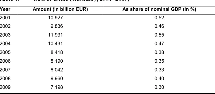
Much of the attention on studies of crime is justified by the sheer magnitude of criminal activities and its associated social costs. Take the case of a burglary. One needs to keep in mind that the costs of such a legal breach are not borne simply by the victim. There are also law-enforcement costs related to determining and apprehending the suspect, as well as the cost of having police personnel in the first place to prevent such crimes. Upon arrest, the legal system also comes into play: lawyers’ fees must be paid as well as judges’ salaries. In jurisdictions with juries, the opportunity costs of members of the jury must also be taken into account. Moreover, there is the expected response of the victim and her neighbors, who will now presumably undertake more security measures such as installing electronic anti-burglary systems or safer windows. Considering the number of crimes committed every year, the associated annual total so-cial cost would be staggering ‒ and this is even without acknowledging the non-pecuniary costs of victimization, such as psychological stress. As a rough measure,

(7)

Table 1 presents the direct cost of crime as estimated by the Federal Criminal Police Office in Germany.

Table 1: Cost of crime (Germany, 2001‒2009)

Year Amount (in billion EUR) As share of nominal GDP (in %)

2001 10.927 0.52

2002 9.836 0.46

2003 11.931 0.55

2004 10.431 0.47

2005 8.418 0.38

2006 8.190 0.35

2007 8.042 0.33

2008 9.960 0.40

2009 7.198 0.30

Source: Polizeiliche Kriminalstatistik: Bundeskriminalamt (2009) and Statistisches Bundesamt Deutschland (2010).

Despite having one of the lowest national crime rates ‒ even for Western European standards ‒ the federal government of Germany has been consciously addressing the issue of criminality within its borders. The contribution of this study is to examine the effects of the programmed military base realignments and closures (BRACs) in Germany ‒ in particular, the effect on criminal activity surrounding the base. Reducing crime is a matter of public policy, and any initiative that contributes to this goal, whether inadvertently or deliberately, requires careful study to guide policymakers. Within the context of the massive reorganization of the German armed forces, it becomes necessary to evaluate the effects of BRACs, not only on defense and strategic grounds, but also on outcomes that are perhaps less obvious to the casual observer. Accounting for the hidden costs and benefits of such a reorganization is of paramount importance in order to avoid basing policy decisions on incomplete information.

(8)

presence of service-members and their dependents as consumers in the local economy, and through the employment of civilian workers.

Given these positive economic influences, it is perhaps surprising that the overall impression gleaned from press reports, particularly from the US, is one of elevated crime within the surrounding community owing to the presence of a base.8

Nevertheless, academic accounts are often more sanguine. Raphael and Winter-Ebmer (2001), for example, argue that while reduced military expenditure may increase social friction by causing unemployment, it has no immediate impact on crime, once other factors, such as demographic composition and alcohol consumption, are controlled for. A case study by Thanner (2006) finds local residents in Maryland even deriving a sense of security from the base and a perceived increase in crime following its closure, attributing this to the loss of the base’s putative deterrence effect.

However, aus dem Moore (2012) shows that the closures of US military bases in Germany reduced drug offenses and rape, although the size of the US bases in Germany were much larger than the German bases in our dataset. Ramstein Air Base of the US Air Force, for example, has about 60,000 military and civilian personnel, about 7 times larger than the largest base in the current paper. In addition, it is difficult to make a comparison with the study of American bases since social cohesion is largely determined by similarities in culture, including language. American military servicemen do not typically share the same culture as the Germans living in communities surrounding the base, which may cause more tension than what one may expect from German military personnel in Germany.

Moreover, the closure and drawdown of German military bases did not result in the unemployment of service personnel. They were relocated to other bases in the country, which means that they were shielded from an unemployment shock. As we mention in Paloyo et al. (2010), in a number of areas where German military bases were closed, the local government took the opportunity to re-service some of the infrastructure, thereby creating employment and perhaps dampening the potential negative impacts on the local economy.

To contribute to this issue, we assembled data from the Federal Criminal Police Office (Bundeskriminalamt), Federal and State Statistical Offices (Statistische Ämter des Bundes und der Länder), and the Federal Ministry of Defense (Bundesministerium der Verteidigung). The econometric problem is that we cannot observe the counterfactual situation, i.e., we do not know how crime rates would have been if a base had not been been present in the community. The closure and realignment procedure, which started in 2001, gives us a unique opportunity to overcome this identification problem, as it provides us with a natural experiment in which bases were shut down

(9)

solely due to military reasons and requirements, without regard for potential outcomes at the community level. A standard fixed-effects regression model is used to account for residual concerns about the potential endogeneity of BRACs, although, as will be emphasized later in Section 5, there is substantial evidence to suggest that planned BRACs were unrelated to the outcome variables of interest. Furthermore, we estimate our regression models over data that have been transformed with geographic information system (GIS) software. More explicitly, we create buffer zones that surround each base to deal with issues associated with using regional data based on politically delineated borders.

2. Young men and crime

The reason we expect a relationship to exist between military bases and the crime rate is that young men commit the majority of crimes, and young men comprise the majority of the military-base population. The German armed forces (Bundeswehr) are composed primarily of men: women comprise a mere 10 percent.9

By and large, crime is disproportionately committed by young men. There are a variety of reasons for this phenomenon, including economic ones. For example, when the economy is in recession, one of the areas of the labor market that is typically and severely affected is the segment populated by young, unskilled labor. For instance, given the existing employment laws in Germany, it is easier for firms to shed themselves of younger workers with shorter tenure. Conscripts ‒ usually young men below the age of 25 ‒ are also generally earning less than the amount they could be earning in the civilian labor market. This reduced earnings capacity in the legal labor market may tip the balance between licit and illicit activities towards the latter, making it more profitable for juveniles and young adults to engage in criminal activity.

In this case, however, we note that the base closures and realignments in Germany did not have a deleterious effect on legal economic opportunities. In previous research (Paloyo et al. 2010), we demonstrate that this adjustment process in Germany did not have an impact on the regional economy, especially in terms of output, employment, and tax revenue (among other economic variables). This is in contrast to the results obtained by aus dem Moore (2012) for US bases, but the characteristics of US bases in Germany were very different from those of domestic German bases, and it would not be an informative comparison, as we have previously mentioned.

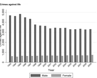
The Bundeskriminalamt in Wiesbaden is responsible for publishing statistics on criminal activity and is the source of our data on crime. In Figures 1(a) and 1(b), we

(10)

plot the total amount of crime and crimes against life known to law enforcement, respectively, for Germany for the period 1993‒2009 and disaggregated by the sex of the offender. With respect to both categories, the number of male offenders dominate the number of female offenders, and even more so when one looks at crimes against life (Straftaten gegen das Leben).

Figure 1: Total crime and crimes against life by sex, 1993‒2009 (Germany)

(a) Total crime

0

5

10

15

20

Tot

al r

ec

or

de

d of

fe

ns

es

(i

n 100

,000

)

1993 1994 1995 1996 1997 1998 1999 2000 2001 2002 2003 2004 2005 2006 2007 2008 2009

Year

(11)

Figure 1: (Continued)

(b) Crimes against life

Source: Polizeiliche Kriminalstatistik: Bundeskriminalamt (2009).

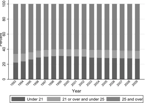
Figures 2(a) to 2(d) show the share of offenders by age group for both total crime and crimes against life and separately calculated for men and women. For both sexes, young people (those below 21 years old) commit a substantial part of total crime (about 25 percent). The percentage is somewhat lower for more violent crimes, such as crimes against life. For those under 25, their share of total offenses hovers a little below 40 percent for both men and women, although it is quite clear that young men commit the majority of crimes that all men commit, and this is a higher share than the crimes committed by young women as a share of crimes committed by all women. Taking into account that criminal activities are, for the most part, supplied by young men, it is therefore worthwhile to ask whether a concentration of such a group, for instance, in a military base, would have an impact on crime in the surrounding community.

0

1,

00

0

2,

00

0

3,

00

0

4,

00

0

5,

00

0

Cr

im

es

aga

in

st

li

fe

1993 1994 1995 1996 1997 1998 1999 2000 2001 2002 2003 2004 2005 2006 2007 2008 2009 Year

(12)

Figure 2: Total crime and crimes against life by age group, 1993‒2009 (Germany)

(a) Total crime, male offenders

(b) Crimes against life, male offenders

0

20

40

60

80

10

0

Pe

rce

nt

1993 1994 1995 1996 1997 1998 1999 2000 2001 2002 2003 2004 2005 2006 2007 2008 2009 Year

Under 21 21 or over and under 25 25 and over

0

20

40

60

80

10

0

Pe

rce

nt

1993 1994 1995 1996 1997 1998 1999 2000 2001 2002 2003 2004 2005 2006 2007 2008 2009 Year

(13)

Figure 2: (Continued)

(c) Total crime, female offenders

(d) Crimes against life, female offenders

Source: Polizeiliche Kriminalstatistik: Bundeskriminalamt (2009).

0

20

40

60

80

10

0

Pe

rce

nt

1993 1994 1995 1996 1997 1998 1999 2000 2001 2002 2003 2004 2005 2006 2007 2008 2009 Year

Under 21 21 or over and under 25 25 and over

0

20

40

60

80

10

0

Pe

rce

nt

1993 1994 1995 1996 1997 1998 1999 2000 2001 2002 2003 2004 2005 2006 2007 2008 2009 Year

(14)

In terms of convictions for crimes committed by employees of the Bundeswehr (among others, conscripts, fixed-term soldiers, and professional soldiers), we obtained data from parliamentary inquiries in 2006 and 2008, which are presented in Table 2.10

Here, we see that the trend in violent crimes committed by employees of the Bundeswehr seems to follow a similar pattern depicted in Figure 1(b). We take advantage of structural reforms, described in depth in the next section, being undertaken in the German Federal Defense Forces to examine the relationship, if any, between the presence of a military base and criminal activity surrounding the base.

Table 2: Convictions for violent crimes of military personnel

Year _Murder _ManslaughterNumber of convictions _{Sex crime} _{Violent crime}

1990 0 3 35 764

1991 2 0 33 620

1992 1 4 33 634

1993 4 1 31 634

1994 0 1 77 719

1995 0 0 28 649

1996 4 3 18 513

1997 1 2 25 507

1998 1 0 26 483

1999 1 1 28 586

2000 2 1 29 480

2001 1 0 18 354

2002 1 2 36 369

2003 2 0 35 339

2004 1 1 32 345

2005 1 0 34 266

2006 0 1 38 281

2007 1 1 28 262

Note: The convictions may refer to offenses committed while not associated with the Bundeswehr.

Source: Deutscher Bundestag Drucksache 16/3168, 16/10164.

(15)

3. The transformation of the German armed forces

For Germany, the threat of a border invasion has all but dissipated. This is due to a number of factors but primarily because the Cold War has ended, and the European Union has established itself as a viable political and economic agglomeration of countries. The security threats faced by Germany (and many other countries in the Western world) now come from substate and stateless terrorist organizations from as far away as Afghanistan and Pakistan. The military deployment strategy that was appropriate to defend Germany against an invasion originating from the other side of the Iron Curtain is now acknowledged to be insufficient to protect Germany and its citizens from organizations that threaten it today.11

In response to these changes, new Defense Policy Guidelines (Verteidigungspolitische Richtlinien) were adopted by the German Parliament in 2003. These guidelines emphasized the transition of the German armed forces from a territorial defense force into one that could be deployed rapidly and internationally to address security concerns abroad. The task of the Bundeswehr now involves “multinational conflict prevention and crisis management operations” while everything else “not conducive to this goal is of secondary importance.”12_{The results of such a}

transformation of the Bundeswehr are evident in the contribution of Germany to multinational military operations. For instance, the Commander of the Regional Command North of the International Security Assistance Force (ISAF) in Afghanistan is German. Next to the US and the UK, Germany is the largest contributor of military personnel to the ISAF. This represents a dramatic shift in Germany’s security policy.

Before the new Defense Policy Guidelines, however, Germany was already embarking on the path to rationalize the Bundeswehr. This is embodied in the proposal of the Federal Ministry of Defense called the Departmental Deployment Concept (Ressortkonzept Stationierung), which was adopted in 2001. This new deployment plan involved a substantial military drawdown, including the reduction of military personnel and the reduction of the military bases located within Germany. The program, which spans the period 2003‒2011, dictates the closure of 187 bases and the reduction of personnel in 177 other bases. With this planned reorganization, the federal government ultimately intends to reduce the total number of active bases from 575 in 2003 to 388 in the year 2011. In Figure 3, we provide a map of the German bases included in our study, and indicate those that closed during the study period.

11_{To be accurate, such an invasion cannot be completely ruled out. Therefore, the}_Bundeswehr_{is being} trans-formed today with this possibility taken into account, which means that should such a “conventional attack” become imminent, the armed forces can be reconstituted quickly to respond to and neutralize the threat. The whole point of the new defense concept can be seen as one that emphasizes flexibility of the Bundeswehr to respond to multiple threats.

(16)

(17)

Former Defense Minister, Karl-Theodor zu Guttenberg, had proposed a plan to even more drastically reduce the size of the Bundeswehr. From its complement of 245,000 soldiers in 2009, zu Guttenberg intended to cut it down to 163,500 over the next few years. The plan also included the suspension of compulsory military service and the transformation of the Bundeswehr into a professional army composed of an all-volunteer force, which is presumably more effective. In addition, the plan raised the average number of military personnel in a base to 900, which means the realignment of personnel and the closure of redundant bases.13

For some bases, downsizing the military complement might prove difficult. Consider the top 10 Gemeinden (municipalities or towns; LAU 2, formerly NUTS 5) by military personnel presented in Table 3. In 2003, the base in Koblenz employed 8,830 persons, which represented about 8 percent of the population in that area in 2003. However, in the same year, the average military complement for a base is about 324 individuals. Thus, to achieve the target, the realignment of personnel will have to be substantial.

Table 3: Top 10 Gemeinden by military personnel complement in 2003

Gemeinde Kreis Personnel population Share in 2003 2007 2003 2007

Koblenz Koblenz 8,830 8,830 0.0819 0.0832

Düsseldorf Düsseldorf 3,020 3,020 0.0053 0.0052

Hammelburg Bad Kissingen 2,490 1,830 0.0228 0.0172

Penzing Landsberg am Lech 2,360 2,360 0.0215 0.0208

Sigmaringen Sigmaringen 2,200 1,670 0.0164 0.0126

Strausberg Märkisch-Oderland 2,200 2,200 0.0115 0.0115

Regensburg Regensburg 2,140 2,140 0.0167 0.0162

Stetten am kalten Markt Sigmaringen 2,080 2,080 0.0155 0.0157

Memmingerberg Unterallgäu 2,036 0 0.0150 0.0000

Kappeln Schleswig-Flensburg 1,950 0 0.0098 0.0000

Source: Stationierungskonzept der Bundeswehr 2004.

(18)

4. Data description

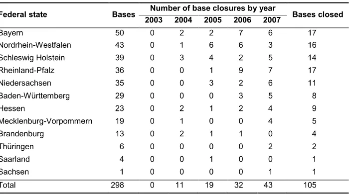
The dataset used in our analysis contains 298 bases, of which 105 were eventually closed.14_{Table 4 presents a timeline of base closures by federal state. The number of}

base closures per year was increasing since the start of the program and culminated in 2007, when 43 bases were closed. Bayern had the highest number of bases at 50 and also the most number of base closures at 17.

Table 4: Timeline of base closures by Federal State

Federal state Bases _{2003 2004 2005 2006 2007}Number of base closures by year Bases closed

Bayern 50 0 2 2 7 6 17

Nordrhein-Westfalen 43 0 1 6 6 3 16

Schleswig Holstein 39 0 3 4 2 5 14

Rheinland-Pfalz 36 0 0 1 9 7 17

Niedersachsen 35 0 0 3 2 6 11

Baden-Württemberg 29 0 0 0 3 5 8

Hessen 23 0 2 1 2 4 9

Mecklenburg-Vorpommern 19 0 1 0 0 4 5

Brandenburg 13 0 2 1 1 0 4

Thüringen 6 0 0 0 0 2 2

Saarland 4 0 0 1 0 0 1

Sachsen 1 0 0 0 0 1 1

Total 298 0 11 19 32 43 105

Source: Stationierungskonzept der Bundeswehr 2004.

The data on crime were obtained from the Polizeiliche Kriminalstatistik published annually by the Federal Criminal Police Office (Bundeskriminalamt 2009).15_Apart

from the total criminal offenses known to law enforcement, the publication also has crime disaggregated by the type of crime. Other socioeconomic variables were drawn from the Federal and State Statistical Offices (Statistische Ämter des Bundes und der Länder 2008). The data are recorded at the Kreis level (NUTS 3), the Kreis being an administrative region in Germany with an average area of 814 sq. km. Information pertaining to the military bases was collected from the Deployment Concept of the

14_{Missing information in any of the covariates used later in the regression analysis necessitated dropping} certain bases from the dataset.

(19)

Federal Armed Forces of Germany (Bundesministerium der Verteidigung 2004). The location information on the bases is provided at the Gemeinde level, the Gemeinde being smaller than the Kreis to which it belongs. Each Gemeinde is located in only one Kreis (i.e., the former's border does not cross the latter’s).

The classification of criminal offenses into various categories is done by the Federal Criminal Police Office. In this study, we use the following specific categories: (i) total crimes (Straftaten insgesamt) comprise all crimes but without offenses against residence, asylum, or free-movement-of-persons regulations (for instance, staying illegally in Germany, having no passport, etc.); (ii) drug-related crimes (Rauschgiftdelikte) are all direct offenses related to illicit drugs: selling, buying, possessing with intent, as well as indirect offenses like robbery and breaking and entering to gain access to drugs or to finance a drug addiction, and driving under the influence of drugs; (iii) violent crimes (Körperverletzung) are murder, manslaughter, rape, assault, threatening with assault or bodily harm, hostage-taking and, in general, all violent exchanges between persons, normally with intent; (iv) breaking and entering (Wohnungseinbruchdiebstahl) includes breaking and entering, stealing or its attempt, and all related offenses, like damaging windows, doors, etc.; (v) stealing from cars (Diebstahl in/aus Kraftfahrzeuge) is actual stealing of cars and stealing from cars with intent (but not related to drugs; otherwise, it would be recorded in drug-related crimes).

In general, violent crime is reserved for more serious cases. The categories are exclusive, i.e., crimes are not counted in more than one group. If a person commits a combination of crimes, say, running over someone to get money for drugs, the most serious offense is recorded. Typically, when a violent crime is committed together with a property crime, the event is counted under the latter category.16_{The list of crimes in}

the dataset is not exhaustive, and in all cases, the sum of the different crime variables that are available does not equal the total number of crimes for a particular area.

The data are spatial in nature, which we take into account by transforming the data first before assembling and preparing it for estimation. Spatially explicit data are becoming increasingly common in demographic research, a development that has thrust the issue of geographic scale into greater prominence. As defined by Reardon et al. (2008:489), geographic scale refers to “the dimensions of identifiable social or physical features of a landscape”. The ability to delineate such features is, of course, circumscribed by the level of spatial aggregation at which the data are measured. When measured at the most disaggregated level, units of observation can be located in space by their exact geographic coordinates, thereby affording a high degree of flexibility in how spatial influences are incorporated into the analysis. In a study of psychoactive substance use, for example, Chaix et al. (2005) take advantage of information on the exact residential location of individuals in the city of Malmö, Sweden using

(20)

coordinates to create circular but non-uniform areas of constant population size centered on each individual.

The data used in the present analysis do not benefit from this degree of precision but are still measured at a sufficiently fine geographic scale to capture economic conditions surrounding the base. Using GIS software, we create buffer zones ‒ uniformly sized circular areas with the base at its center ‒ to take into account the information from the surrounding Kreise. To do this, we first draw a buffer zone around the centroid of the Gemeinde where the base is located.17_{The area of overlap for each}

Kreise contained in this buffer zone is calculated and then divided by the total area of the buffer zone. The resulting ratio is used to weight the information assigned to that Kreis. This allows us to compute a weighted sum that summarizes the available information from the surrounding Kreise of a particular base. This approach, also favored by Banzhaf and Walsh (2008) for applications to US census data, incorporates the information from the home and surrounding Kreise. It ameliorates some of the difficulties associated with the so-called modifiable areal-unit problem (Openshaw 1984), such as the use of varying and arbitrarily sized spatial units of analysis.

Consider, for instance, the case depicted in Figure 4. Here, the Gemeinde (crosshatch pattern) is located at the edge of its home Kreis (gray). If we were to take into account ‒ using the method described above ‒ that it shares the border with two other Kreise, we would calculate total crime associated with that military base as follows:

total_crime_𝑗weighted=� �_{total_area_buffer}overlap_area𝑖

𝑗×total_crime𝑖� 3

𝑖=1

,

where 𝑖 and 𝑗 are the Kreis (where the base is located) and buffer zone, respectively. For our purposes, we set the radius of the buffer zones to 12 km and 20 km. This allows us to roughly determine how far from the centroid the effect, if any, travels.

(21)

Figure 4: GIS-based calculation of the variables, 12-km buffer zone

(22)

One drawback in processing the data this way is the assumption that the surfaces are isotropic, i.e., that the magnitude of the effect emanating from the centroid is invariant with respect to direction. This is problematic when the politically delineated borders are the result of natural features such as mountains and rivers, over which the effects may not necessarily propagate as easily as over plains. Therefore, we also estimate our model using untransformed data, i.e., without the buffer-zone transformation, to check the robustness of our results. We also present estimates using a 20-kilometer buffer to gauge the extent to which the modifiable areal-unit problem may bear on the results.

While we have every reason to believe that the decision pertaining to which bases will be closed is based purely on strategic grounds, we nevertheless perform an equality-of-means test between areas where bases closed and areas where bases stayed open to show that these bases do not differ in their observed characteristics. This implies that, at least in terms of the observable elements, the places with base closures are comparable to those places without base closures. We perform the test for two years: specifically, 2003, where the bases are first observed in the dataset, and 2007, where they are last observed. The results are displayed in Table 5. They indicate that there is no substantial difference between the areas where a base closed and the areas where bases remained open, which makes a comparison between the two groups more credible.

Table 5: Equality-of-means test, 2003 and 2007

Variable

2003

p-value

2007 _p -value With

closure closure No closure With closure No Panel A: 12-km buffer zone

Crime rate (all crimes) × 10,000 635.70 648.65 0.5521 621.50 628.32 0.7319 Annual real household income 17,074.11 17,330.70 0.2698 19,941.70 20,299.21 0.3812

Unemployed ÷ population 0.0454 0.0483 0.3026 0.0389 0.0410 0.3604

Foreigners ÷ population 0.0615 0.0646 0.4352 0.0611 0.0639 0.4625

Males aged 15‒25 ÷ population 0.0603 0.0602 0.9173 0.0605 0.0599 0.2064

(23)

Table 5: (Continued)

Variable With 2003 p-value 2007 _valuep -closure closure No closure With closure No Panel B: 20-km buffer zone

Real GNP (in 100,000) 51.3316 54.9975 0.5034 48.3141 51.4668 0.5354

Panel C: Untransformed data

Real GNP (in 100,000) 45.1935 50.1877 0.3111 42.4847 46.6024 0.3616

Observations 105 193 105 193

Note: Income and GNP are in euro. The p-values are based on two-sided t-tests.

Source: Authors’ calculation.

In light of the seminal studies of Becker (1968) and Ehrlich (1973), we hypothesize that variables that increase either economic well-being or the likelihood of arrest serve as deterrents to crime. More precisely, anything that increases the returns to licit activities relative to illicit activities should reduce the propensity to commit crime. Variables that relate to these opportunities are also therefore included in the regression model described in detail below. These include real GNP and relative disposable income. Conversely, variables that undermine social cohesion or economic security are hypothesized to increase the crime level, such as the percentage of foreigners and of the unemployed.18_{In addition, we expect positive relationships between (i) the number of}

foreigners and crime and (ii) the number of young men and crime owing to a higher incidence of economic duress and exclusion from the labor market within these groups. Being located in East Germany is also hypothesized to be associated with higher levels of crime, given a sustained period of depressed economic conditions in that region. Finally, as large populations have generally been found to be associated with higher

(24)

crime, we expect a positive coefficient for this variable (United States Department of Justice 2009).19

5. Estimation strategy and results

To identify the impact of adjustments in the size of military bases, including closures, we estimate the following regression model:

ln𝑦𝑖𝑡=𝛼+𝛿DP𝑖𝑡+𝛃′𝐱𝑖𝑡+𝛉′𝐳𝑡+𝑒𝑖𝑡, (1)

where 𝑦𝑖𝑡 is a generic outcome variable (here, total crime and its subcategories) for unit

𝑖 in year 𝑡, DP𝑖𝑡 is the number of military personnel in thousands (Dienstposten), 𝐱𝑖𝑡 is a

vector of control variables, 𝐳𝑡 is a vector of unit-invariant year fixed effects, and 𝑒𝑖𝑡 a

stochastic disturbance term with the usual properties. The coefficients 𝛼, 𝛿, 𝛃, and 𝛉 are a set of parameters and parameter vectors to be estimated. The coefficient of interest is 𝛿, which represents the causal effect of BRACs on criminal activity surrounding the base.

We exploit the panel structure of the dataset by augmenting Equation (1) with a time-invariant and buffer-specific (or, in the case of the untransformed data, Kreis-specific) fixed effect:

ln𝑦𝑖𝑡=𝛼+𝛿DP𝑖𝑡+𝛃′𝐱𝑖𝑡+𝛉′𝐳𝑡+𝜙𝑖+𝑒𝑖𝑡. (2)

The term 𝜙𝑖 represents unobserved community-specific characteristics that affect

the outcome variable but do not change over time. For instance, certain geographic characteristics are captured by 𝜙𝑖. Allowing for the possibility that this term is

correlated with 𝑒𝑖𝑡, we proceed to apply a fixed-effect transformation to the data to

eliminate any residual biases.

As noted in the introduction, one important institutional aspect is that the decision to close or downsize a military base was made purely on strategic grounds that were unrelated to the intensity of criminal activity surrounding the selected base. As opposed to the US experience, where the execution of the base closures was substantially influenced by the demands of the local communities in which bases were located

(25)

(Brauer and Marlin 1992), the military drawdown in Germany was not altered by popular or political considerations. The planning period of the scheme covered two government periods and both major political parties. The overarching shift from territorial defense to expeditionary warfare drove the decision-making process. No planned base closure was taken back or altered, and there was no formal process for local communities to appeal the decision of the federal government.20_{This peculiar}

aspect of the implementation of the Deployment Concept of the armed forces in Germany enables us to recover the causal impact of BRACs.

The outcome variables used in this study are the following: total crime, breaking and entering, automobile-related crime, violent crime, and drug-related crime. These are all set to logarithm so that the coefficients can be directly interpreted as semi-elastic elements. The control variables contained in 𝐱𝑖𝑡 are an indicator variable that equals 1

for East Germany and 0 otherwise (this is eliminated in the fixed-effects model through the within transformation), real GNP in million euro (lagged one year), the percentage of the unemployed in the community, the share of foreigners in the community, the percentage of young men (aged 15‒25 years old) in the community, household disposable income relative to the national mean (lagged one year), and population in ten thousands. All control variables are measured at the level of the Kreis.

Estimates of the coefficients based on Equations (1) and (2) are presented in Tables 6 and 7, respectively. Both tables use the GIS-transformed data with the 12-kilometer buffer. The appendix presents results using a 20-12-kilometer buffer as well as the untransformed data. Based on OLS regressions, we note that the presence of military personnel has no evident impact on crime levels across most of the measured categories. The one exception is drug-related crimes, with a point estimate [standard error] of 0.041 [0.022]. Specifically, the coefficient suggests that a 1,000-person increase in military personnel is associated with a 4.1-percent increase in drug-related crimes ‒ a seemingly small effect that, as presented below, is not robust to the inclusion of fixed effects.

(26)

Table 6: OLS regression results (12-km buffer)

Dependent variables (to logarithm) Total

crime Breaking and entering

Auto-related

crime

Violent

crime related Drug-crime

Military personnel ÷ 1,000 0.021 0.026 0.040 0.017 0.041*

[0.013] [0.024] [0.025] [0.015] [0.022]

Real GNP ÷ 1,000,000 (lagged) −0.031*** −0.080*** −0.081*** −0.020** −0.002

[0.011] [0.018] [0.018] [0.009] [0.011]

Household relative income

(lagged) −0.976***[0.223] −1.168***[0.399] −1.164***[0.430] −0.761***[0.194] −1.672***[0.348]

Share of foreigners 3.805*** 3.389** 4.364*** 2.601*** 8.452***

[0.975] [1.558] [1.624] [0.817] [1.139]

Share of unemployed 5.338*** 10.200*** 13.416*** 5.396*** −4.546**

[1.469] [2.659] [3.035] [1.219] [1.996]

Share of men aged 15‒25 −21.804***−58.139*** −40.227*** −19.192*** −3.144

[3.722] [6.336] [7.733] [3.301] [4.899]

Population ÷ 10,000 0.059*** 0.091*** 0.095*** 0.048*** 0.041***

[0.004] [0.006] [0.006] [0.003] [0.005]

East Germany 0.102 −0.078 −0.237 −0.167** 0.046

[0.100] [0.171] [0.215] [0.082] [0.128]

Constant Yes Yes Yes Yes Yes

Year fixed effects Yes Yes Yes Yes Yes

F-statistic 80.88 72.19 87.51 126.49 100.70

R2 _0.8562 _0.7552 _0.7519 _0.8317 _0.6834

Observations 1,192 1,192 1,192 1,192 1,192

Note: The dependent variables are the number of offenses per crime category and are expressed in logarithm. Bracketed numbers are robust standard errors clustered at the buffer level. * p < 0.10, ** p < 0.05, *** p < 0.01.

Of the remaining coefficient estimates, the majority that is statistically significant has signs that are consistent with expectations based on the existing literature. Economic well-being, as measured by real GNP and relative disposable income, is negatively associated with crime, while higher unemployment has a positive association. Also confirming expectations, regions with a higher percentage of foreigners have higher crime levels. (Entorf and Spengler 2000) These are also consistent with the results obtained by Messner et al. (2013:1015) in their “exploratory spatial data analysis” ‒ that is, areas within Germany with “high robbery and assault rates tend to be those with comparatively high levels of socioeconomic deprivation”.

(27)

term. On the whole, the qualitative findings do not vary markedly. With regard to military personnel, the results confirm the impression gleaned from the OLS estimates that this variable is not significantly correlated with crime. The most notable discrepancy is seen for the coefficient estimate for the number of young men, which now has the expected positive coefficient in each of the models.

Table 7: FE regression results (12-km buffer)

Auto-related

crime

Violent

Military personnel ÷ 1,000 −0.016 −0.030 −0.022 0.005 0.057

[0.016] [0.058] [0.069] [0.013] [0.042]

Real GNP ÷ 1,000,000

(lagged) −[0.015] 0.014 −[0.053] 0.152*** −[0.058] 0.098* [0.020] 0.033* [0.036] 0.087** Household relative income

(lagged) −[0.283] 0.446 −[0.976] 1.643*

−1.823*

[1.059] −0.092[0.375] −[1.158] 4.129***

Percentage of foreigners 3.677** 16.788*** 6.762 3.688** 16.734***

[1.542] [5.310] [5.725] [1.766] [5.730]

Percentage of unemployed 2.021*** −1.136 2.420 2.931*** 3.346

[0.745] [2.788] [2.829] [1.018] [3.149]

Percentage of men aged 15‒

25 6.608*** [1.394] 3.205** [5.097] 11.863** [5.155] 3.768** [1.995] 7.468 [5.384]

Population ÷ 10,000 0.019*** 0.090*** 0.086*** −0.003 −0.083***

[0.010] [0.028] [0.034] [0.021] [0.025]

F-statistic 20.05 18.58 58.99 40.13 16.91

Within R2 _0.1861 _0.1046 _0.3284 _0.2585 _0.1908

Observations 1,192 1,192 1,192 1,192 1,192

Note: The dependent variables are the number of offenses per crime category and are expressed in logarithm. Bracketed numbers are robust standard errors. * p < 0.10, ** p < 0.05, *** p < 0.01.

6. Conclusion

(28)

bases are located. Among the effects plausibly instigated by a base closure is a change in the intensity of criminal activities. To the extent that the personnel who populate the bases are largely comprised of young men ‒ the demographic segment most prone to criminal activity ‒ it is conceivable that the closures would reduce crime rates. Given the substantial financial and psychic costs of crime, such an outcome would register as a clear benefit to communities otherwise concerned about the economic impacts of the closures. This paper has attempted to empirically address this issue by assembling a panel dataset that links regional crime rates to military base complements and socioeconomic variables.

While our analysis confirms the significance of many of the correlates of crime identified elsewhere in the literature, including the population, unemployment rate, the presence of young men, and measures of local economic well-being, we find no evidence for an association of crime with the military bases. This conclusion holds over different estimation methods and different scales of analysis.

(29)

References

Angrist, J.D. (1990). Lifetime earnings and the Vietnam era draft lottery: Evidence from social security administrative records. American Economic Review 80(3): 313–336. doi:10.3386/w3514.

aus dem Moore, J.P. (2012). Essays on the Impact of Economic Shocks in Local Labor Markets. Doctoral Dissertation. Berlin: Humboldt University of Berlin, Faculty of Economics.

aus dem Moore, J.P. and Spitz-Oener, A. (2012). Bye bye GI: The impact of the US military drawdown on local German labor markets. SFB 649 Discussion Paper No. 2012-024.

Banzhaf, H.S. and Walsh, R.P. (2008). Do people vote with their feet? An empirical test of Tiebout’s mechanism. American Economic Review 98(3): 843–863. doi:10.1257/aer.98.3.843.

Bauer, T.K., Bender, S., Paloyo, A., and Schmidt, C.M. (2012). Evaluating the labor-market effects of compulsory military service. European Economic Review 56(4): 814–829. doi:10.1016/j.euroecorev.2012.02.002.

Becker, G.S. (1968). Crime and punishment: an economic approach. Journal of Political Economy 76(2): 169–217. doi:10.1086/259394.

Brauer, J. and Marlin, J.T. (1992). Converting resources from military to nonmilitary uses. Journal of Economic Perspectives 6(4): 145–164. doi:10.1257/jep.6.4.145. Bundeskriminalamt (2009). Polizeiliche Kriminalstatistik 2009. Wiesbaden:

Bundeskriminalamt.

Bundesministerium, der Verteidigung (2004). Die Stationierung der Bundeswehr in Deutschland. Berlin: Bundesministerium der Verteidigung.

Bushway, S., Cook, P., and Phillips, M. (2012). The overall effect of the business cycle on crime. German Economic Review 13(4): 436–446. doi:10.1111/j.1468-0475.2012.00578.x.

(30)

Droff, J. and Paloyo, A.R. (2014). Assessing the regional economic impacts of defense activities: A survey of methods. Journal of Economic Surveys. doi:10.1111/ joes.12062.

Ehrlich, I. (1973). Participation in illegitimate activities: a theoretical and empirical investigation. Journal of Political Economy 81(3): 521–568. doi:10.1086/ 260058.

Entorf, H. and Spengler, H. (2000). Socioeconomic and demographic factors of crime in Germany: evidence from panel data of the German states. International Review of Law and Economics 20(1): 75–106. doi:10.1016/S0144-8188(00) 00022-3.

Galiani, S., Rossi, M., and Schargrodsky, E. (2011). Conscription and crime: Evidence from the Argentine draft lottery. American Economic Journal: Applied Economics 32(2): 119–136.

Gottfredson, M.R. and Hirschi, T. (1990). A General Theory of Crime. Stanford, CA: Stanford University Press.

Grogger, J. (1998). Market wages and youth crime. Journal of Labor Economics 16(4): 756–791. doi:10.1086/209905.

Jacob, B.A. and Lefgren, L. (2003). Are idle hands the devil’s workshop? Incapacitation, concentration, and juvenile crime. American Economic Review 93(5): 1560–1577. doi:10.3386/w9653.

Levitt, S.D. (1998). Juvenile crime and punishment. Journal of Political Economy 106(6): 1156–1185. doi:10.1086/250043.

Lindo, J. and Stoecker, C. (2014). Drawin into violence: Evidence on “what makes a criminal” from the Vietnam draft lotteries. Economic Inquiry 52(1): 239–258. doi:10.1111/ecin.12001.

Merton, R.A. (1949). Social Theory and Social Structure. New York: The Free Press. Messner, S.F., Teske, R.H.C., Baller, R.D., and Thome, H. (2013). Structural covariates

of violent crime rates in Germany: Exploratory spatial analyses of Kreise. Justice Quarterly 30(6): 1015–1041. doi:10.1080/07418825.2011.645862. Openshaw, S. (1984). The Modifiable Areal Unit Problem. Norwich, UK: Geo Books. Öster, A. and Agell, J. (2007). Crime and unemployment in turbulent times. Journal of

(31)

Paloyo, A.R., Vance, C., and Vorell, M. (2010). The regional economic effects of military base realignments and closures in Germany. Defence and Peace Economics 21(5‒6): 567‒579. doi:10.1080/10242694.2010.524778.

Raphael, S. and Winter-Ebmer, R. (2001). Identifying the effect of unemployment on crime. Journal of Law and Economics 44(1): 259–283. doi:10.1086/320275. Reardon, S.F., Matthews, S.A., O’Sullivan, D., Lee, B.A., Firebaugh, G., Farrell, C.R.,

and Bischoff, K. (2008). The Geographic Scale of Metropolitan Racial Seggregation. Demography 45(3): 489–514. doi:10.1353/dem.0.0019.

Rohlfs, C. (2010). Does combat exposure make you a more violent or ciminal person? Evidence from the Vietnam draft. The Journal of Human Resources 45(2): 271– 300.

Semyonov, M., Gorodzeisky, A., and Glikman, A. (2012). Neighborhood ethnic composition and resident perceptions of safety in European countries. Social Problems 59(1): 117–135. doi:10.1525/sp.2012.59.1.117.

Siminski, P., Ville, S., and Paull, A. (2013). Does the military train men to be violent criminals? New evidence from Australia’s conscription lotteries. IZA Discussion Paper No. 7152.

Statistische Ämter, des Bundes und der Länder (2008). Statistik Regional 2008 (DVD). Statistische Ämter des Bundes und der Länder.

Thanner, M.H. (2006). Military base closure effects on a community: the case of Fort Ritchie Army Garrison and Cascade, Maryland. [PhD Thesis]. College Park, MD: University of Maryland.

(32)

Appendix: Supplemental regression tables

Table A1: OLS regression results (20-km buffer)

Auto-related

crime

Violent

Military personnel ÷ 1,000 0.014 0.021 0.019 0.016 0.046**

[0.013] [0.022] [0.022] [0.014] [0.023]

Real GNP ÷ 1,000,000 (lagged) −0.033*** [0.012] −0.084*** [0.017] −0.092*** [0.016] −0.024** [0.011] 0.001 [0.010] Household relative income

(lagged) −0.580* [0.322] −0.674 [0.441] −0.497 [0.546] −0.198 [0.303] −1.366*** [0.409]

Percentage of foreigners 3.112*** 3.103** 3.445** 1.237 8.066***

[1.030] [1.542] [1.660] [0.840] [1.240]

Percentage of unemployed 6.667*** 13.435*** 17.189*** 5.898*** −3.878**

[1.651] [2.723] [3.209] [1.434] [1.946]

Percentage of men aged 15-25 −18.045*** [4.468] −54.022*** [6.308] −37.907*** [8.238] −16.625*** [3.858] 1.241 [4.697]

Population ÷ 10,000 0.060*** 0.091*** 0.097*** 0.051*** 0.041***

[0.003] [0.005] [0.006] [0.003] [0.004]

East Germany 0.017 −0.303* −0.446** −0.151 −0.006

[0.109] [0.172] [0.217] [0.099] [0.115]

F-statistic 127.81 102.07 119.73 199.94 134.27

R2 _0.8794 _0.7831 _0.7830 _0.8591 _0.7240

Observations 1,192 1,192 1,192 1,192 1,192

(33)

Table A2: FE regression results (20-km buffer)

Auto-related

crime

Violent

Military personnel ÷ 1,000 −0.010 −0.021 −0.012 0.002 0.036

[0.014] [0.053] [0.064] [0.011] [0.037]

Real GNP ÷ 1,000,000 (lagged) −0.003 [0.016] −0.095 [0.050] −0.079 [0.055] 0.065*** [0.013] 0.054* [0.030] Household relative income

(lagged) −0.445 [0.298] 2.510** [1.025] −1.742 [1.190] −0.208 [0.373] −5.374*** [1.080]

Percentage of foreigners 4.416*** 19.783*** 4.257 5.463*** 19.747***

[1.430] [4.582] [5.182] [1.592] [5.053]

Percentage of unemployed 2.381*** −0.547 4.019 3.764*** 2.142

[0.702] [2.628] [2.884] [0.886] [2.962]

25 [1.342] 5.776*** [4.913] 2.979 [5.000] 8.900* [1.797] 3.017* 11.123** [4.922]

Population ÷ 10,000 0.036*** 0.024*** 0.052*** −0.015** −0.010

[0.005] [0.009] [0.015] [0.006] [0.010]

F-statistic 38.28 30.67 77.48 58.41 19.27

Within R2 _0.3094 _0.1260 _0.3619 _0.3140 _0.2646

Observations 1,192 1,192 1,192 1,192 1,192

(34)

Table A3: OLS regression results (Untransformed data)

Auto-related

crime

Violent

Military personnel ÷ 1,000 0.042* 0.030 0.079** 0.031* 0.063**

[0.021] [0.032] [0.039] [0.018] [0.025]

Real GNP ÷ 1,000,000 (lagged) 0.001 [0.007] 0.019 [0.012] −0.011 [0.010] −0.002 [0.007] -0.007 [0.012] Household relative income

(lagged) −0.734*** [0.156] −0.583* [0.334] −0.671** [0.335] −0.846*** [0.166] −1.359*** [0.294]

Percentage of foreigners 2.366*** 1.055 1.616 2.268*** 6.751***

[0.527] [1.106] [1.103] [0.638] [1.102]

Percentage of unemployed 7.053*** 10.812*** 13.819*** 6.913*** −2.253

[1.620] [2.843] [3.045] [1.492] [2.079]

25 −11.845*** [3.261] −42.054*** [6.563] −22.976*** [7.015] −11.877*** [3.498] [5.637] 1.510

Population ÷ 10,000 0.048*** 0.073*** 0.074*** 0.042*** 0.040***

[0.003] [0.005] [0.005] [0.003] [0.005]

East Germany −0.050 −0.209 −0.393* −0.330** −0.108*

[0.111] [0.199] [0.219] [0.102] [0.152]

F-statistic 68.65 53.55 78.70 66.73 38.92

R2 _0.7973 _0.6830 _0.6859 _0.7497 _0.5360

Observations 1,192 1,192 1,192 1,192 1,192

Note: The dependent variables are the number of offenses per crime category and are expressed in logarithm. Bracketed numbers are robust standard errors clustered at the buffer level. * p < 0.10, ** p < 0.05, *** p < 0.01.

(35)

Table A4: FE regression results (Untransformed data)

Auto-related

crime

Violent

Military personnel ÷ 1,000 −0.015 [0.019] −0.043 [0.060] −0.007 [0.081] 0.000 [0.015] 0.079 [0.048] Real GNP ÷ 1,000,000

(lagged) −0.012 [0.012] −0.052 [0.047] −0.019 [0.051] −0.032* [0.019] 0.023 [0.035] Household relative income (lagged) −0.246 [0.205] −0.810 [0.948] −0.794 [1.002] −0.360 [0.358] −2.408** [1.010] Percentage of

foreigners [1.740] 3.243* 13.372** [6.323] [6.156] 8.145 [1.718] 2.178 10.496 [6.676] Percentage of

unemployed [0.828] 1.686** −[3.051] 0.968 [3.026] 1.959 [0.988] 3.152*** [3.119] 1.806 Percentage of men

aged 15‒25 [1.757] 6.680*** [5.960] 5.251 13.380** [6.237] [1.899] 4.462** [5.882] 6.589

Population ÷ 10,000 0.011 0.063 −0.002 0.014 −0.139**

[0.019] [0.062] [0.071] [0.025] [0.058]

F-statistic 15.03 9.85 34.97 21.62 10.57

Within R2 _0.1349 _0.0729 _0.2649 _0.1674 _0.1197

Observations 1,192 1,192 1,192 1,192 1,192

(36)