in the population sciences published by the Max Planck Institute for Demographic Research Konrad-Zuse Str. 1, D-18057 Rostock · GERMANY www.demographic-research.org
DEMOGRAPHIC RESEARCH
VOLUME 27, ARTICLE 12, PAGES 339-364
PUBLISHED 28 AUGUST 2012
http://www.demographic-research.org/Volumes/Vol27/12/ DOI: 10.4054/DemRes.2012.27.12
Research Article
Educational differences in chronic conditions
and their role in the educational differences in
overall mortality
Ruben Castro
© 2012 Ruben Castro.
This open-access work is published under the terms of the Creative Commons Attribution NonCommercial License 2.0 Germany, which permits use, reproduction & distribution in any medium for non-commercial purposes, provided the original author(s) and source are given credit.
1 Introduction 340 1.1 Decomposing the differentials in overall mortality 341
2 Model, data and methodology 342
2.1 The condition’s prevalence versus its influence on overall mortality 342 2.2 Interpreting P as the prevalence of the chronic condition 343
2.3 Decomposition analysis 344
2.4 Data 344
2.5 Measures 345
2.6 Estimate of rates and differentials 346
2.6.1 Rates 346
2.6.2 Differentials 347
3 Results 347
3.1 Descriptive statistics 347
3.2 Estimated incidence, baseline, and excess mortality rates by chronic
condition 349 3.3 Educational differences in chronic conditions and their role in overall
mortality 350
3.4 Analysis by gender 352
4 Discussion 354
5 Acknowledgments 355
References 356
Educational differences in chronic conditions and their role in the
educational differences in overall mortality
Ruben Castro1
Abstract
Demographers use different models to decompose the prevalence of given health conditions. This article discusses how these models can help us understand the ways in which these conditions affect overall mortality. In particular, this framework can be used to understand the role that any given condition plays in producing differences in overall mortality across populations. The empirical analysis in this study focuses on chronic conditions as factors behind elderly US citizens’ differences in overall mortality across educational levels. The analysis of differences by education level shows that while the prevalence differences of chronic conditions is mostly the outcome of
incidence differences, regarding overall mortality differences, the role of chronic
conditions is equally channelled through incidence and excess mortality differences.
1. Introduction
Existing research on the relationship between education and mortality presents robust evidence that death rates are higher among individuals with lower levels of education.2
This phenomenon is observable during an individual’s whole life span3 and increases
over time.4 Furthermore, the correlation exists at all income distribution levels (Smith
2005.)
Although part of the mortality and health gradient has not been attributed to any specific factor,5 there is an extensive body of research dealing with the wide range of
conditions that allegedly underlie the education-mortality relationship. In fact, the vast majority of conditions that influence mortality are also linked to education, in terms of their incidence rates and their associated excess mortality rates.
Several studies focus on decomposing differentials in the prevalence of a given
condition across population groups, which are seen as the outcome of differentials on the condition’s incidence and excess mortality. This study emphasises that this analysis can be extended to the differentials of overall mortality, with the aim of better
understanding the impact of any given condition in overall mortality across gender, location, race or educational level.
Demographers and epidemiologists make use of multi-state life tables6 to simulate
prevalence dynamics. These enable the differences in the prevalence of any condition across populations to be simulated as the outcome of differences in underlying incidence and mortality rates. Examples of this are Leveille et al. (2000) and Melzer et al. (2001) for gender and educational differences in the prevalence of disability, and
2 For example, see Goldman (2001).
3 During childhood, there is evidence of the effect of socioeconomic level on health, as shown in Case et al.
(2002). In this case, the effect seems to be caused by household conditions and intrauterine nutrition. At the other extreme, a socioeconomic gradient is also found among elderly people in numerous studies; such as those by Zhu and Xie (2007) and Huisman et al. (2004) who present evidence from various countries. It is worth noting that for elderly people, the gradient begins to moderate, as shown by Crimmins (2005).
4 Singh and Siahpush (2002), Singh and Yu (1995). Pappas et al. (1993) show that “among whites and blacks
of both sexes, the differences in mortality according to educational level were greater in 1986 than in 1960” (results section).
5 De Vogli et al. (2007) made the following observation: “Although [major mechanisms proposed to explain
the health gradient] contribute to explaining population health variations, large gradients are found even in societies with favorable circumstances with relation to health determinants and health status” (page 143). Hayward et al. (2000) studied the relationship between socioeconomic level and racial disparity for chronic conditions and concluded that “the racial health disparity is spread across all health domains, and socioeconomic conditions, not health risk behaviors, are the primary causes of the racial stratification of health” (p. 910).
6Multi-state life tables are also known as increment-decrement life tables. They are models for processes
Lipscombe and Hux (2007) for time differences in the prevalence of diabetes in Canada. The idea behind this analysis has been extended even further, for example, to the study of car accidents (where the “states” are defined by the action of driving in Dellinger et al. 2002); the study of the existence of disability given a chronic condition (Freedman et al. 2007) or to better portray the dynamics of entry and exit from states of depression through life (Patten and Lee 2005).
Another extension is to simulate the dynamics of overall mortality, which arises from the same model as that of prevalence, as discussed in Section 2.1, 2.2, and 2.3. In other words, the demographic rates behind the prevalence of any given condition are also the components behind the condition’s influence on the overall mortality rate. One important lesson is that while one component may have the greatest influence on prevalence, it may not be the most important way in which the condition affects overall mortality.
The empirical contribution of this study focuses on the role of chronic conditions in US educational differences in mortality. The most common causes of death in the developed world are associated with chronic diseases. The U.S. Centers for Disease Control and Prevention states that, according to Kung et al. (2008): “7 out of 10 deaths among Americans each year are from chronic diseases and heart disease, cancer and strokes account for more than 50% of all deaths each year”. Furthermore, growth in the prevalence of chronic conditions has been projected, from 118 million Americans in 1995 to 171 million by 2030 (Wu and Green 2000).
There is a large body of literature that deals with educational differentials in diagnosed chronic diseases. Depending on the settings of each study, low levels of education as opposed to high levels of education are found to be associated with as much as twice the risk of both the incidence of, and mortality from, the chronic conditions included in this study (with the exception of cancer). These results underlie the education differentials in prevalence. They also underlie the impact of chronic conditions on the educational differences in mortality.
1.1 Decomposing the differentials in overall mortality
Throughout this study, I conceptualise overall mortality as the sum of base line mortality experienced by all individuals plus the excess mortality experienced above the base line by individuals with the chronic condition under analysis.
It is important to note that even though exactly the same model and the same rates that decompose prevalence also decompose overall mortality, the lessons from the former cannot be simply applied to the latter. Higher excess mortality is unambiguously associated with lower prevalence, at least in models of reasonable simplicity, but it is ambiguously associated with overall mortality, because the higher excess mortality raises overall mortality on the one hand but also makes the condition less prevalent on the other.
The empirical analysis focuses on education differentials in six chronic conditions among the elderly, as included in the Health and Retirement Study (HRS). These are, in order of prevalence, hypertension, heart attacks, diabetes, cancer, strokes and lung disease. These conditions have virtually no reverse transition, which simplifies the discussion, and are also of widespread interest for researchers. The decomposition is performed with the aim of providing a measurement of the relative importance of base line mortality, chronic conditions’ incidence and chronic conditions’ excess mortality, in terms of explaining the magnitudes of education differentials on overall mortality and prevalence. Each chronic condition is analysed separately according to its “implied stationary population”; which is the population that would emerge if demographic rates (births, base line mortality, transition and excess mortality) were to remain constant over an extended period.
Section 2 discusses the model, data and methodology. Section 3 presents the results, including an analysis by gender, and the last section discusses the results.
2. Model, data and methodology
2.1 The condition’s prevalence versus its influence on overall mortality
For clarity of interpretation, the mortality of individuals with a chronic condition is described here as “excess mortality”, which means the mortality gap that exists with comparable individuals without a chronic condition. It should be noted that the main reason for differentiating between “excess mortality” and “mortality” is a question of interpretation.
individuals; M+E, the annual mortality of unhealthy individuals; and T, the transition rate into unhealthiness. It is easy to prove that overall annual mortality (OM) can be expressed in the Equation 17, where P represents the proportion of total person years
lived in an unhealthy state. P is a relatively simple function of T, M and E.
OM depends on two flux variables, M and E, and one stock variable, P. Since P is a function of T, then T leads indirectly to OM. P is also a function of E, so E also leads indirectly to OM. In addition, E leads directly to OM, since OM is a direct function of E:
OM=M+P·E (1)
OMT=PT·E (2)
OME=PE·E+P (3)
Formally, OMT and OME in Equation 2 and 3 are the derivatives of OM with
regard to T and E respectively. OMT’s sign is positive because PT is necessarily positive
(see Appendix 2). OME’s sign is ambiguous because P is positive, while PE is negative
(see Appendix 2). So, while the effects of T and E on P are positive and negative respectively, their effects on OM are positive and ambiguous, respectively. For this reason, the interplay of T and E behind P can be substantially different from the interplay behind OM.
2.2 Interpreting P as the prevalence of the chronic condition
The cohort described above can be followed not only for one year, but for its entire life cycle; which allows age-specific M, T and E rates to be calculated. The lifetime overall mortality can still be expressed as in Equation 1, though the dynamics of the process makes the algebra of P more complex.
The empirical analysis in this study focuses on the stationary population scenario, in which all rates (the birth rate, and the observed cross-sectional age-specific values of M, T and E) are constant over time. This synthetic cohort perspective is less data-demanding than a decomposition of the observed P and OM over a given period of time, which requires the whole history of past and present age-specific rates. The
7OM is defined as the number of deaths over the number of person years. These quantities can be split into
stationary population scenario offers an insightful conceptual perspective: person years lived between ages x and x+n, as implied by a life table, are equivalent, in the stationary
population, to the number of persons between those ages (Preston et al. 2000). Therefore P, the ratio of person years, becomes the ratio of persons; i.e. the prevalence.
2.3 Decomposition analysis
This study computes the multi-state life tables associated with different values of baseline mortality and chronic conditions’ incidence and excess mortality rates. The equations of the multi-state model are discussed in Appendix 1. In essence, in a given interval of time, each individual has a probability of dying, which is higher if the individual has a chronic condition. Individuals without chronic conditions are also at risk of transitioning into the category of “having a diagnosed chronic condition” during an interval of time. No reverse transition is assumed.
First, a reference group is defined. Its multi-state life table is computed based on age-specific estimates of M, T and E for this group. The values of P (which, in the stationary population associated with the multi-state life table, is interpreted as the prevalence) and overall mortality are calculated. Second, a comparison group is defined. The differences between the reference and comparison groups are decomposed using Das Gupta (1993). Thus, differences in P and overall mortality are decomposed as differences in M, T and E.
The analysis does not include gender at any stage. However, the results from gender-specific analysis, as shown in Section 3.4, were substantially consistent with the results discussed in the following sections.
2.4 Data
The data used in this study comes from the Health and Retirement Survey (HRS) and the Study of Assets and Health Dynamics among the Oldest Old survey (AHEAD), which are jointly provided by the University of Michigan. All individuals included in the “Wave 2 release,” that is, interviewed in 1994 (HRS) and 1993 (AHEAD), are included in this study.8 Only the few individuals under the age of 50 in Wave 2 are
8 The data includes sampled individuals’ spouses. The AHEAD cohort contains people born in 1923 or
excluded from the sample. Individuals included in Wave 2 are followed until Wave 6 in 2004.
This panel data was selected because of the sample sizes (over 17,000 individuals) and the remarkable quality of the health measures. More importantly, this survey has a long follow-up period of over 10 years. The sample also focuses on the older population, which, when conducting mortality analysis, acquires greater statistical power. Also, occurrences of death have been doubly verified using data from the National Death Index.9
2.5 Measures
Different health conditions are included in the data sets. Articles on healthy life expectancies, for example, use diseases, pain, cognition and mobility (Mathers et al. 1999), as well as self-assessed general health (Doblhammer and Kytir 2001), institutionalized population and disability (Crimmins and Saito 2001), and self-reported diseases (Banks et al. 2006). The concepts discussed in this study can be applied to any of those measures.
The empirical exercise to be conducted here focuses on chronic diseases. As included in the Health and Retirement Study (HRS), education differentials in six chronic conditions among the elderly (namely hypertension, heart attacks, diabetes,10
lung disease, cancer and strokes) are analysed according to their prevalence and implications for overall mortality. All of them are documented to have high or moderate prevalence in recent years in the US,11 and to be associated with a higher mortality rate.
There is much to explore regarding the demographic dynamics behind their prevalence and especially their implications for overall mortality. Psychiatric illness and arthritis were not included because they seem to have a lower correlation with mortality.
Diagnoses of chronic diseases are self-reported, as are most health variables included in surveys. Nonetheless, it is a fairly objective measure, as it is based on
9 HRS administrative staff repeatedly checks the National Death Index for all individuals, even if they are not
currently being interviewed. In this study, individuals are considered alive unless there is some evidence to the contrary, even if they are not being interviewed. This is not done in the case of health state, where individuals not being interviewed are considered missing.
10 However, the link between diabetes and mortality might largely be due to cardiovascular disease. In the
words of Chaturvedi et al. (1998), “we confirm the existence of an inverse socioeconomic mortality gradient in diabetic people and suggest that this is largely due to conventional cardiovascular risk factors”.
11 According to the data used in this study, the prevalence at age 50-54 is 31%, 9%, 9%, 4%, 4% and 2% for
responses to the question: “Has a doctor ever told you that….”12 As does occur with
other health variables, a self-reported diagnosis is likely to contain education-related, non-random error. In particular, a problem of under diagnosis might arise if
less-educated individuals are less likely to visit a doctor, the doctor is less likely to diagnose them or they are less likely to report the diagnosis in the survey. This is a potential limitation to the empirical application in this study.
This article focuses on education differentials because education can be usefully interpreted as a measure of socioeconomic status (Lynch 2003). In addition, educational levels are established early in life, which minimises reverse causation issues. Furthermore, Smith (2005) analyses different data sets, including HRS and AHEAD, and concludes that financial socioeconomic variables (household income, wealth and even exogenous changes in wealth) “are either not related, or at best weakly related, to the future onset of disease over the time span of eight years” (page 12) Additional education, says Smith (2005), “is strongly and significantly predictive of the new onset of major and minor disease” (page 12). Education is measured in this study as “years of education,” recoded on a scale from 1 to 3: 1 (0/11), 2 (12) and 3 (13+). Level 2 is the reference group.
2.6 Estimate of rates and differentials
2.6.1 Rates
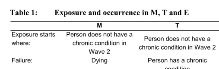
The age-specific M, T and E rates of reference group individuals (individuals with 12 years of education) are estimated directly from follow up data in HRS and AHEAD as events over exposure. Table 1 presents a brief description of the M, T and E.
The sample data used in this study contains only people aged 50 or over. Mortality prior to age 50 is a rare event, at least among more recent cohorts in the U.S., and therefore this limitation might not be crucial to the study of the implications of M and E. However, in the case of T, an earlier onset of a chronic condition is certainly not uncommon: of those interviewed in the 1994 Wave of HRS and AHEAD, about 37% of respondents aged 50 to 54 reported having been diagnosed with at least one of the illnesses considered in this study. The prevalence of chronic conditions at age 50 is approximated in this study as the outcome of T alone.
12 The exact wording of the question depends on whether this is a first interview, whether the person being
Table 1: Exposure and occurrence in M, T and E
M T M+E
Exposure starts where:
Person does not have a chronic condition in
Wave 2
Person does not have a chronic condition in Wave 2
Person has a chronic condition in any Wave
Failure: Dying Person has a chronic
condition
Dying
Exposure ends with no failure if:
Person has a chronic condition or reaches
Wave 7
Person dies or reaches Wave 7 without a chronic
condition
Person reaches Wave 7
2.6.2 Differentials
Due to sample sizes, education- and age-specific rates are estimated with a high degree of uncertainty. For greater precision, it is assumed that the rates ratio (hazard ratio) between the reference group and the comparison group is constant across age intervals. Naturally, flexibility is lower in this case. One way to estimate the hazard ratio is to bring together the data of individuals of all ages to calculate the OM or P ratios, though this would also reflect the different age composition of each educational group. A better option is a Cox model (Cox 1972) with age as the time variable, which also has the advantage of not assuming any particular shape for the underlying hazard. No covariates are included. Regarding the differences in the T rate before age 50, the differences in prevalence at age 50 are directly included in the simulations, and interpreted as the outcome of ΔT alone.
3. Results
3.1 Descriptive statistics
with more than 12 years, respectively.13 The proportion of those with at least one
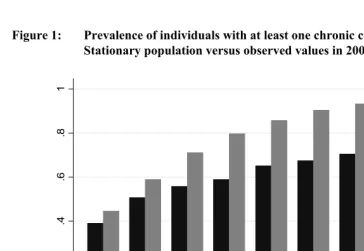
chronic condition at the start of the following period, as shown in Figure 1, rises from 37% in the 50-54 year age group to a maximum of 70% in the 80-84 year age group.
Figure 1: Prevalence of individuals with at least one chronic condition: Stationary population versus observed values in 2002
0
.2
.4
.6
.8
1
50-54 55-59 60-64 65-69 70-74 75-79 80-84 85-89 90+ Obseved Multi-state life table
Observed Stationary population
Source: Author’s calculations.
It is important to emphasise that this study analyses the stationary population scenario (where rates are constant over time). In contrast, the observed proportion with
a chronic condition is the outcome of current and past values of M, T and E. The observed proportions will only be consistent with the proportions implied by the multi-state life table where the current and past values of those rates are equal. Figure 1 shows
13Census 2000´s official reports (Bauman and Graf 2003) show that 32.3% of individuals aged 25 and above
the prevalence of individuals with at least one chronic condition at the start of the follow-up period; and clearly differs from the same prevalence where it corresponds to the stationary population.
3.2 Estimated incidence, baseline, and excess mortality rates by chronic condition
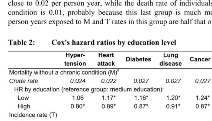
With reference to the magnitudes of the rates, Table 2 contains the “crude” rates of M, T and E. Age-specific values of those rates can be found in Appendix 3 (the crude rates are the ratio of the total number of failures over the total exposed person years). The death rate of individuals without the specified chronic condition is in all cases very close to 0.02 per person year, while the death rate of individuals without any chronic
condition is 0.01, probably because this last group is much more selective (in fact, person years exposed to M and T rates in this group are half that of the other groups).
Table 2: Cox's hazard ratios by education level
Hyper- tension
Heart
attack Diabetes
Lung
disease Cancer Stroke
Any of them Mortality without a chronic condition (M)a
Crude rate 0.024 0.022 0.027 0.027 0.027 0.026 0.010
HR by education (reference group: medium education):
Low 1.06 1.17* 1.16* 1.20* 1.24* 1.21* 1.10
High 0.80* 0.89* 0.87* 0.91* 0.87* 0.90* 0.76*
Incidence rate (T)
Crude rate 0.042 0.024 0.014 0.009 0.013 0.012 0.074
HR by education (reference group: medium education):
Low 1.10* 1.13* 1.48* 1.30* 0.88* 1.16* 1.10*
High 0.93 1.01 0.87* 0.79* 1.09 0.91 0.97
Excess mortality rate (E)a
Crude rate 0.039 0.063 0.053 0.072 0.062 0.094 0.042
HR by education (reference group: medium education):
Low 1.73* 1.20* 1.14* 1.09 1.23* 1.09 1.22*
High 1.33 0.90* 1.20 0.89 0.93 0.87 0.97*
* p-value<=5%. T refers to the rate of transition from having no chronic condition to having one (or more). E refers to the excess mortality among individuals with a chronic condition. The last category, “Any of them,” refers to individuals with one or more of the chronic conditions included in this study. The difference in person years exposed to T and M arises because it is assumed, when calculating the baseline mortality, that people dying shortly after a survey maintain their last observed health state, which adds person years to the calculation of the baseline mortality rate.a For individuals with chronic conditions, Cox's hazard ratios
In Table 2, the chronic conditions appear in order of prevalence. As expected, higher prevalence occurs with higher incidence rates and lower excess mortality rates. The excess mortality rate is heterogeneous, ranging from 0.04 for hypertension, to 0.09 for strokes; and therefore the mortality of individuals with a chronic condition goes from approximately 0.06 to 0.11 per person year. Regarding incidence rates, hypertension is the most likely transition (0.04 per person year), while lung disease is the least likely (0.01 per person year).
Table 2 also contains the Cox model estimate of hazard ratios. In 16 out of 21 Cox regressions, the ratio in the low to medium education group is higher than ratio in the high to medium education group. All the hazard ratios show a negative relationship between education and the incidence and mortality rates of chronic conditions, except in three cases: 1) Excess mortality for hypertension produces a U-shape on the graph. Unfortunately there are no comparable figures in the literature, but De Gaudemaris et al. (2002) found an inverted U-shape for prevalence, which is coherent with a U-shape for excess mortality (however, the levels of education used in De Gaudemaris et al. (2002) are different from the ones in this study). 2) Excess mortality for diabetes produces a U-shape. A comparable figure is found in Dray-Spira et al. (2010), where the mortality of adults with and without diabetes according to education level is shown on page 1202, and the difference corresponds to excess mortality. For non-cardiovascular diseases (the most common ones) there is a U-shape; while in the case of cardiovascular disease there is no U-shape. This discrepancy could be related to age profiles (US population in Dray-Spira et al. 2010, the implied stable population in this study) and data sets (National Health Interview Survey from 1986 to 1996 in Dray-Spira 2010). 3) Cancer incidence rates have a positive association with education. This is also found in previous literature: Smith (2005) points out that, “In all cases except cancer (which looks like an equal opportunity disease) the effects of schooling are preventative against disease onset”. Meanwhile, Johnson et al. (2010) found that a link between higher prevalence and a lower education level existed for only two cancers out of thirteen.
However, even where the hazard ratios of T and E appear to be substantially similar, their influence on prevalence and overall mortality can be very different.
3.3 Educational differences in chronic conditions and their role in overall mortality
analysed next. The same conclusions can be made from the case of high versus medium levels of education, as discussed in Appendix 4, though in this case it is important to emphasise that point estimates of hazard ratios show low significance (see Table 2) and therefore there is considerable uncertainty regarding their estimation.
The total education differential corresponds exactly to the sum of each component of the decomposition. Each chronic condition is analysed separately. The results in Table 3 should be interpreted from a stationary-population perspective, as they pertain to hypothetical cohorts that pass through each of the age-specific rates estimated from the data over a lifetime.
Regarding the education differential in the prevalence of chronic conditions, the component associated with ∆M (the education differential in the baseline mortality) is very low. This is an intuitive result, since higher values of baseline mortality reduce the size of both the “healthy” and the “unhealthy” groups.
On the other hand, the component associated with ∆T is substantially greater than that of ∆E in all cases except for cancer. In other words, it is apparent that incidence rather than excess mortality rates explain most of the education differentials in the prevalence of chronic conditions. Even in the case of the two most prevalent chronic conditions, hypertension and heart attacks, where the hazard ratios for E are bigger than those for T (see Table 2), the latter are apparently the most influential.
There are two reasons for this result. First, the incidence rates, unlike mortality rates, exert their influence from the early stages of life. Hoffman et al. (1996) concluded that the majority of persons with chronic conditions are not elderly. Second, incidence reduces the “healthy” group and enlarges the “unhealthy” one; while excess mortality only reduces the “unhealthy” group.
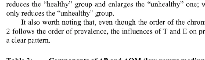
It also worth noting that, even though the order of the chronic conditions in Table 2 follows the order of prevalence, the influences of T and E on prevalence do not show a clear pattern.
Table 3: Components of ∆P and ∆OM (low versus medium educational levels)
∆P = Education differentials in prevalencea
Total ∆M ∆T ∆E
Hypertension 7.4 -0.4 9.1| -1.4
Heart attack 3.7 -0.9 5.3 -0.7
Diabetes 8.6 -0.5 9.5 -0.4
Lung disease 3.1 -0.3 3.6 -0.2
Cancer -1.4 -0.8 -0.1 -0.5
Stroke 0.8 -0.7 1.7 -0.2
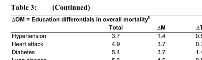
Table 3: (Continued)
∆OM = Education differentials in overall mortalityb
Total ∆M ∆T ∆E
Hypertension 3.7 1.4 0.5 1.8
Heart attack 4.9 3.7 0.7 0.5
Diabetes 5.4 3.7 1.4 0.3
Lung disease 5.6 4.6 0.8 0.2
Cancer 5.8 5.5 0.0 0.3
Stroke 5.6 5.0 0.5 0.1
Any of them 3.8 1.0 0.9 1.9
*The decompositions are based on Das Gupta (1993). M refers to the baseline mortality rate that people with and without the chronic conditions experience. T refers to the rate of transition from not having a chronic condition to having a chronic condition. E refers to the excess mortality among individuals with a chronic condition. The last category, “any of them” refers to individuals with one or more chronic conditions. a: Prevalence is measured in percentage points. b: mortality is measured as number of deaths per thousand person years. Components may not add up to the total due to approximations.
For the case of overall mortality, the situation is different. First, ∆Ms are the most influential components, meaning that no chronic condition can explain most of the educational differences in mortality by itself. This occurs, to an extent, because the effect of incidence on overall mortality is not direct and occurs throughout P; while the effect of excess mortality on overall mortality, on the other hand, is partially self-counteracted by its diminishing effect on prevalence, as discussed earlier.
Second, the contribution of each chronic condition to the differential in overall morality is more evenly distributed between ∆T and ∆E. Furthermore, in some cases excess mortality seems more influential than its incidence, as is the case for hypertension, where excess mortality is clearly more influential than its incidence.
In Tables 2 and 3, each chronic condition is analysed separately. To include all chronic conditions in one analysis, an “Any of them” category, meaning individuals with any one or more of the chronic conditions, is added to Tables 2 and 3. The results for this category follow the same lines as before, with incidence more important than excess mortality in the case of ∆P but not in the case of ∆OM.
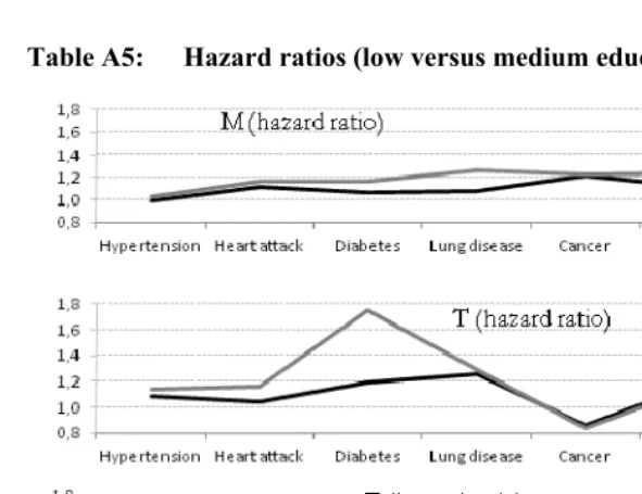
3.4 Analysis by gender
and prevalence of chronic conditions (Case and Paxson 2005), and there is a gender gap in educational attainment for the 1931-1941 cohort (Folger and Nam 1967).
One way to explore whether or not the results are equally true for both men and women is to repeat the entire analysis separately for men and for women. Table A5 in Appendix 5 shows the low-to-medium education hazard ratios from Table 2, but calculated for men and women separately. Despite some gender differences (the ratios are somewhat bigger for women, particularly in the case of base line mortality), there is a general similarity. Then, replicating the same methodology as used in the rest of this study, the stationary population scenarios (rates constant over time) were simulated and the results are shown in Table 4:
Table 4: Components of ∆P and ∆OM (low versus medium educational levels) by gender
Men Women
ΔM ΔT ΔE ΔM ΔT ΔE
∆P = Education differentials in prevalencea
Hypertension 0 7 -2 0 10 -2
Heart attack -1 2 -1 -1 7 -1
Diabetes 0 2 -1 0 13 0
Lung disease 0 4 -1 0 3 0
Cancer -1 -1 0 -1 0 -1
Stroke 0 2 0 -1 1 0
Any of them -1 2 -1 0 11 -1
∆OM = Education differentials in overall mortalityb
Hypertension 0 1 3 0 1 2
Heart attack 3 0 0 3 1 1
Diabetes 2 0 1 3 2 0
Lung disease 3 1 1 5 1 0
Cancer 6 0 0 4 0 1
Stroke 4 1 0 4 0 0
Any of them 3 0 1 -1 1 2
*Source: Author’s calculations. All notes under Table 3 apply.
4. Discussion
Demographers use different models to decompose the prevalence of given health conditions. This article discusses how such models can also help us to understand the way in which these conditions affect overall mortality.
A useful first step is to conceptualise mortality as the sum of base line mortality plus the excess mortality that arises once a chronic condition is diagnosed. Otherwise, it is harder to interpret, for example, how much the lower mortality of a highly-educated individual is actually linked to a lower incidence of hypertension, because their mortality is lower even in the absence of hypertension.
The prevalence dynamics are different from the overall mortality dynamics. For instance, the excess mortality associated with any given condition makes the condition less prevalent, but the conclusion remains ambiguous with regard to overall mortality. Higher excess mortality produces higher overall mortality, but at the same time it makes the condition less prevalent. The case of cancer is instructive. The lower incidence and higher excess mortality of individuals in the group with lower education suggests a relatively lower prevalence but a relatively higher overall mortality.
The model in this article is based on the stationary population associated with a group of underlying demographic rates. There are three demographic rates in the model: baseline mortality, the incidence of a given condition, and the excess mortality associated with the condition. The differences between two stationary populations can be decomposed as the outcome of differences on each of the three demographic rates. This framework can be used to understand the role that any given condition plays in generating differences in overall mortality across populations.
This idea highlights the fact that, with regard to policy, the relative importance of differentials on incidence and excess mortality rates depends on the target of interest, prevalence or overall mortality.
An empirical analysis is developed next, focussing on the difference that the educational level of elderly US citizens makes to chronic conditions. Chronic conditions rank first in US causes of death. The incidence and excess mortality rates associated with chronic conditions differ by educational level, as is also the case with the mortality rates not associated with chronic conditions. Understanding how those differentials operate is fundamental, not only for understanding the prevalence differentials, but also to understanding how chronic conditions are partially responsible for the educational differences in overall mortality. Six chronic conditions among elderly US citizens are analysed.
The gender-specific analysis shows substantially the same results. Nevertheless, a useful extension of this study would be to analyse gender differences, rather than educational differences.
The case of hypertension is also instructive. Its low-to-medium education incidence ratio is lower than its excess mortality ratio. In fact, its excess mortality ratio is the highest of all the chronic conditions. Yet, incidence is the main mechanism
behind the ∆P for hypertension. At the same time, excess mortality is the main
mechanism by which hypertension influences ∆OM.
Results show that education differentials in the prevalence of chronic conditions are barely influenced by differences in baseline mortality. This is an intuitive result, since higher values reduce the size of both the “healthy” and the “unhealthy” group. Also, it is not surprising that incidence rates explain most of the educational differences in the prevalence of chronic conditions. The conceptual section of this study shows that incidence changes the size of both the “healthy” and the “unhealthy” groups, while excess mortality changes only the latter.
One empirical limitation of this study is the use of data about individuals aged 50 or over. No mortality is assumed before that age and, though mortality rates before the age of 50 probably play a minor role, this omission overstates the role of differentials on incidence rates. Another limitation is under-diagnosis among the less-educated individuals, which probably overstates the estimated mortality of healthy individuals and understates the rate of transition into unhealthiness. Finally, the study does not explore whether changes in rates during the 10-year examination period may introduce bias in the results. Nevertheless, the same results are evident using only half the data.
5. Acknowledgments
References
Banks, J., Marmot, M., Oldfield, Z., and Smith, J. (2006). Disease and disadvantage in the United States and in England. Journal of the American Medical Association.
295(17): 2037-2045. doi:10.1001/jama.295.17.2037.
Bauman, K. and Graf, N. (2003). Educational Attainment: 2000. Washington, DC: US Census Bureau.
Case, A., Lubotsky, D., and Paxson, C. (2002). Economic status and health in childhood: The origins of the gradient. American Economic Review. 92(5):
1308–1334. doi:10.1257/000282802762024520.
Case, A. and Paxson, C. (2005). Sex differences in morbidity and mortality.
Demography 42(2): 189-214. doi:10.1353/dem.2005.0011.
Chaturvedi, N., Jarrett, J., Shipley, M., and Fuller, J.H. (1998). Socioeconomic gradient in morbidity and mortality in people with diabetes: Cohort study findings from the Whitehall Study and the WHO multinational study of vascular disease in diabetes. British Medical Journal 316: 100-105. doi:10.1136/bmj.316.7125.100.
Cox, D.R. (1972). Regression models and life tables. Journal of the Royal Statistical Society Series B34(2): 187-220.
Crimmins, E.M. (2005). Socioeconomic differentials in mortality and health at the older age. Genus 61(1): 163-178.
Crimmins, E.M. and Saito, Y. (2001). Trends in healthy life expectancy in the United States, 1970–1990: Gender, racial, and educational differences. Social Science Medicine 52(11): 1629–1641. doi:10.1016/S0277-9536(00)00273-2.
Das Gupta, P. (1993) Standardization and Decomposition of Rates: A User’s Manual. Washington, DC: U.S. Bureau of the Census, Current Population Reports (Series P–23, No 186).
De Gaudemaris, R., Lang, T., Chatellier, G., Larabi, L., Lauwers-Cancès, V., Maître, A., and Diène, E. (2002). Socioeconomic inequalities in hypertension prevalence and care: The IHPAF study. Hypertension 39: 1119–1125. doi:10.1161/ 01.HYP.0000018912.05345.55.
De Vogli, R., Gimeno, D., Martini, G., and Conforti, D. (2007). The pervasiveness of the socioeconomic gradient of health. European Journal of Epidemiology 22(2):
Dellinger, A., Langlois, J., and Li, G. (2002). Fatal crashes among older drivers: Decomposition of rates into contributing factors. American Journal of Epidemiology 155(3): 234-241. doi:10.1093/aje/155.3.234.
Doblhammer, G. and Kytir, J. (2001). Compression or expansion of morbidity? Trends in healthy-life expectancy in the elderly austrian population between 1978 and 1998. Social Science and Medicine 52(3): 385-391. doi:10.1016/S0277-9536(00) 00141-6.
Dray-Spira, R., Gary-Webb, T., and Brancati, F. (2010). Educational disparities in mortality among adults with diabetes in the U.S. DiabetesCare. 33(6):
1200-1205. doi:10.2337/dc09-2094.
Folger, J. and Nam, C. (1967). Education of the American Population. Washington,
DC: Census Monograph.
Freedman, V., Schoeni, R., and Martin, L. (2007). Chronic conditions and the decline in late-life disability. Demography 44(3): 459-477. doi:10.1353/dem.2007.0026.
Goldman, N. (2001). Social inequalities in health: Disentangling the underlying mechanisms. Annals of the New York Academy of Sciences 954: 118-139. doi:10.1111/j.1749-6632.2001.tb02750.x.
Hayward, M.D., Crimmins, E.M., Miles, T.P., and Yang, Y. (2000). The significance of socioeconomic status in explaining the race gap in chronic health conditions.
American Sociological Review 65(6): 910-930. doi:10.2307/2657519.
Hoffman, C., Rice, D., and. Sung, HY. (1996). Persons with chronic conditions: their prevalence and costs. JAMA 276(18): 1473-1479. doi:10.1001/jama.1996. 03540180029029.
Huisman, M., Kunst, AE., Andersen, O., Bopp, M., Borgan, J.-K., Borrell, C., Costa, C., Deboosere, P., Desplanques, G., Donkin, A., Gadeyne, S., Minder, C., Regidor, E. Spadea, T., Valkonen, T., and Mackenbach, J.P. (2004). Socioeconomic inequalities in mortality among elderly people in 11 European populations. Journal of Epidemiology and Community Health. 58: 468–475. doi:10.1136/jech.2003.010496.
Johnson, S., Corsten, MJ., McDonald, JT., and. Gupta, M. (2010). Cancer prevalence and education by cancer site: Logistic regression analysis. Journal of otolaryngology-head and neck surgery 39(5):555-560.
Leveille, S., Penninx, B., Melzer, D., Izmirlian, G. and Guralnik, JM. (2000). Sex differences in the prevalence of mobility disability in old age: The dynamics of incidence, recovery, and mortality. J Gerontol B PsycholSciSocSci 55(1): S41–
S50. doi:10.1093/geronb/55.1.S41.
Lipscombe, L. and Hux, J. (2007). Trends in diabetes prevalence, incidence, and mortality in ontario, canada 1995–2005: A population-based study. Lancet
369(9563): 750–756. doi:10.1016/S0140-6736(07)60361-4.
Lynch, S.M. (2003). Cohort and life-course patterns in the relationship between education and health: A hierarchical approach. Demography 40(2): 309-331. doi:10.1353/dem.2003.0016.
Mathers, C.D., Sadana, R., Salomon, J.A., Murray, C.J., and Lopez, A.D. (1999). Healthy life expectancy in 191 countries. The Lancet 357(9269): 1685-1691. doi:10.1016/S0140-6736(00)04824-8.
Melzer, D., Izmirlian, G., Leveille, S., and Guralnik, J.M. (2001). Educational differences in the prevalence of mobility disability in old age: The dynamics of incidence, mortality, and recovery. J Gerontol B PsycholSciSocSci 56(5): S294–
S301. doi:10.1093/geronb/56.5.S294.
Pappas, G., Queen, S., Hadden, W., and Fisher, G. (1993). The increasing disparity in mortality between socioeconomic groups in the United States, 1960 and 1986.
The New England Journal of Medicine 329(2): 103-109. doi:10.1056/NEJM199 307083290207.
Patten, S. and Lee, R. (2005). Describing the longitudinal course of major depression using Markov models: Data integration across three national surveys. Population Health Metrics 3: 11. doi:10.1186/1478-7954-3-11.
Preston, S., Heuveline, P., and Guillot, M. (2000) Demography: Measuring and Modeling Population Processes. Malden, Mass: Blackwell Publishers.
Singh, G.K. and Siahpush, M. (2002). Increasing inequalities in all-cause and Cardiovascular mortality among US adults aged 25–64 years by area socioeconomic status, 1969–1998. International Journal of Epidemiology 31(3):
600-613. doi:10.1093/ije/31.3.600.
Smith, J. (2005). Unraveling the SES-health connection. Aging, Health and Public Policy: Demographic and Economic Perspectives 30: 108-132.
Wu, S.-Y. and Green, A. (2000). Projection of Chronic Illness Prevalence and Cost Inflation. RAND Corporation.
Appendix
A1. Multi-state model
The formulae used in the study are detailed here. Generic chronic conditions have been assumed, using the terms “healthy” and “unhealthy” to represent individuals with and without the chronic condition, respectively. Age intervals of one year are used. At the beginning of each age interval, shown using a, the number of healthy and unhealthy
individuals are written as lh,a and lu,a. During that interval, there is an age-specific
probability that a healthy individual will die during the year (qh,a), an age-specific
probability that an unhealthy individual will die during the year (qu,a), and an
age-specific probability that a healthy individual will become unhealthy during the year (qt,a). Only one event can happen during one interval, that is, healthy individuals do not
make the transition into unhealthiness and then die during the same interval. No reverse transition is assumed.
As discussed in Preston et al. (2000), the transition probabilities are shown according to age-specific mortality rates among healthy individuals (Ma), excess
mortality among unhealthy individuals (Ea) and the transition rate into unhealthiness
(Ta):
qh,a = Ma/(1+(Ma+Ta)/2) (1.1)
qt,a = Ta /(1+(Ma+Ta)/2) (1.2)
qu,a = (Ma+Ea)/(1+(Ma+Ea)/2) (1.3)
The expressions for the numbers of survivors and person years lived depend on the assumption for the underlying instantaneous forces of mortality and transition. Given
that one-year intervals are used in this study, different assumptions will probably not substantially change the results. It is assumed here that events happen half way through the interval to facilitate derivations. Therefore the person years and number of individuals alive at each age and health state are:
lh,a =lh,a-1(1-qh-qt) (1.4)
lu,a =lu,a-1(1-qu)+ lh,a-1(qt) (1.5)
PYh,a = lh,a-1(1-qh-qt)+ lh,a-1(qh+qt)/2 (1.6)
The minimum age for the exercise in this study is 50 years. The initial proportion of unhealthy individuals at that age is estimated from the unhealthy proportion in the 50-54 age interval as observed in the data.
A2. Derivatives of P
The goal of this Appendix is to prove that the derivative of P is unambiguously positive with respect to T and unambiguously negative with respect to E.
A cohort subject to the same M, T and E rates every year has been assumed until the 100th year, at which time the cohort is basically extinct. The T rate has been assumed to only increase by ΔT in year x. The derivatives of PYh,x and PYu,x with
respect to T are:
d(PYh,x)/dT = lh,x-1(-dqh/dT-dqt/dT)/2 <0 (1.8)
d(PYu,x)/dT = lh,x-1(dqt/dT)/2 >0 (1.9)
It is fairly straightforward to prove that dqt/dT is positive and (-dqh/dT-dqt/dT) is
negative. Therefore in year x the effect of ΔT will reduce the healthy person years lived
and increase the unhealthy ones. Thus the x-specific P will increase. In addition, lh,x+1
decreases and lu,x+1 increases, thus the (x+1)-specific P will also increase; indeed, it can
be proven that each of the future lh and lu will experience the same kind of change,
implying a higher n-th P. Thus, the overall P will be higher.
If T increases by Δ in all years, instead of only in one, then the effect is cumulative. Consequently dP/dT is positive. Similarly, this conclusion can be extended to a-specific M, T and E rates.
The effect of ΔE is simpler, because it influences only one of the three probabilities (qh,a, qt,aandqu,a). It is assumed that the E rate only increases by ΔE in year x. The derivatives of PYh,x and PYu,x with respect to T are:
d(PYh,x)/dE = 0 (1.10)
d(PYu,x)/dE = lu,a-1(-dqu/dE) <0 (1.11)
It is fairly straightforward to prove that -dqu/dT is negative. Given that only
Therefore (x+1)-specific P decreases. Similarly, it can be proven that each of the future
lu will experience the same kind of change, and will therefore have a lower
year-specific P. Thus, the overall P will be lower. If E increases by Δ in all years, then the effect is cumulative. Consequently dP/dE is negative. Again, this conclusion can be extended to a-specific M, T and E rates.
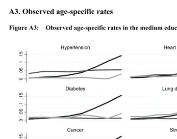
A3. Observed age-specific rates
Figure A3: Observed age-specific rates in the medium education group
0
.0
5
.1
.1
5
0
.0
5
.1
.1
5
0
.0
5
.1
.1
5
50-54 60-64 70-74 80-84 50-54 60-64 70-74 80-84
Hypertension Heart attack
Diabetes Lung disease
Cancer Stroke
M T E
Age intervals
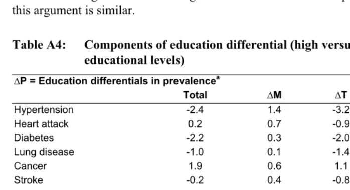
A4. The analysis of the high versus medium educational levels
The body of the article contains the analysis of the low versus medium educational levels. This appendix contains the analysis of the high versus medium educational levels, which is displayed in Table A4. The results of the latter case are, to a large extent, consistent with those found in Table 3. The signs of the effects are opposite because the high-to-medium comparison goes in the opposite direction to the low-to-medium one. For example, the contribution of baseline mortality to overall mortality is positive in Table 3, because baseline mortality accounts for some of the higher mortality observed among individuals with lower education. The same contribution is negative in Table 4, because baseline mortality accounts for some of the lower mortality observed among individuals of high education. For the decomposition of prevalence, this argument is similar.
Table A4: Components of education differential (high versus medium educational levels)
∆P = Education differentials in prevalencea
Total ∆M ∆T ∆E
Hypertension -2.4 1.4 -3.2 -0.7
Heart attack 0.2 0.7 -0.9 0.4
Diabetes -2.2 0.3 -2.0 -0.5
Lung disease -1.0 0.1 -1.4 0.3
Cancer 1.9 0.6 1.1 0.2
Stroke -0.2 0.4 -0.8 0.3
Any of them -0.9 1.0 -2.1 0.2
∆OM = Education differentials in overall mortalityb
Hypertension -4.1 -4.6 -0.2 0.7
Heart attack -2.8 -2.5 -0.1 -0.2
Diabetes -3.0 -3.0 -0.3 0.3
Lung disease -2.6 -2.1 -0.3 -0.2
Cancer -2.9 -3.0 0.2 -0.1
Stroke -2.9 -2.5 -0.2 -0.2
Any of them -3.1 -2.6 -0.2 -0.3
A5. Hazard ratios (low-to-medium educational levels) for men and
women
Table A5: Hazard ratios (low versus medium educational levels) by gender