A Novel System-Level Calibration Method for Gimballed Platform IMU Using Optimal Estimation

© Iranian Aerospace Society, Summer - Fall 2012

J

Journal of

A S T

Aerospace Science and Technology

1 Introduction

IMU is the heart of the inertial navigation system. Its function is to supply acceleration signals which are or can be resolved into components of the desired coordi-nate system [1]. IMU conventionally is a platform which contains three accelerometers mounted on a platform. This platform stays stable in a desired coordinate ref-erence frame. In order to isolate this platform from the vehicle maneuvering, it is usually supported by gimbals

A Novel System-Level Calibration Method for Gimballed Platform IMU

Using Optimal Estimation

H. Darwish Alshaddadi

1

_{, M.R. Arvan and A.R. Vali}

2

An accurate calibration of inertial measurement unit errors is increasingly im-portant as the inertial navigation system requirements become more stringent. Developing calibration methods that use as less as possible of IMU signals has 6-DOF gimballed IMU in space-stabilized mode is presented. It is considered as held stationary in the test location incorporating 15 different error sources, including accelerometers bias, scale factor error, gyros drift, initial alignment error, and IMU case installation error. Using kinematic relations between IMU platform, IMU body, and IMU platform centered inertial reference frame, six differential equations of the only system-level IMU velocity and gimbal angle are derived. Then the extracted model is validated for error-free case using Sim-Mechanics MATLAB SIMULINK tools to evaluate the introduced mathematical model. Simulation results for 24 hours point out the correctness of the devel-oped model in error-free case. The IMU error analysis methodology incorporates ! "# ! gimbal angle measurements taken during one and a half hour with 9 platform at-titudes test to estimate IMU error sources. Without the need to install IMU at ro-tating table, different platform attitudes are achieved using consequent rotations of gimbals. IMU error sources estimation is accomplished off-line. This paper describes the design and test results of a new gimballed IMU calibration method without using a rotating table, and error model development methodology formu-lated to support the design and test of EKF algorithm and two optimal smoothers: forward-backward and RTS. Results obtained from EKF implementation indicate that the technique is comprehensive and accurate, and requires less specialized test equipments. Also, results show that constant states are not smooth-able. Keywords: Gimballed IMU, space-stable IMU, EKF,- RTS, forward-backward.

1. Malek-Ashtar University of Technology (MUT),Tehran, Iran 2. [email protected], [email protected], [email protected]

which allow the housing the full freedom of motion about the platform. For platform isolation three gyros are mounted with the accelerometers on the platform. Any attempt of the platform to rotate will be sensed by one or more of the gyros and correction signals will be sent to the appropriate gimbal servo motor.

The arrangement of the gimbals varies from system

gimbal is mounted on the second or pitch gimbal which is in turn mounted on the third or roll gimbal [2], Figure 1. No matter how the vehicle maneuvers, the pickoff

on the middle gimbal measures pitch, and that on the output set.

Figure 1. Schematic of a gimballed inertial measurement unit [2]

Accelerometers triad mounted on the platform !-ference between the acceleration of the vehicle and the earth gravitational acceleration coordinated in a suit-able reference frame. In some IMU types, accelerom-eters output signals are not available at system-level, where they are integrated internally and corresponding velocity signals are accumulated as the second IMU output set [3].

Figure 2. Real gimballed inertial measurement unit

In Figure 1 the picture of a real gimballed inertial measurement unit with transparent case is shown.

"!

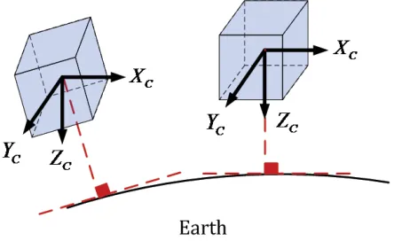
-commanded and the accelerometers measure the specif-ic force whspecif-ich is proportional to the difference between the inertial referenced acceleration and the earth grav-itational acceleration [1, 2], Figure 3. The commanded platform angular velocity will be ideally equal to the !!

#!!$"%&'! model is presented in [10], incorporating all nonlinear-ities torque such as 2-DOF gimbal inertia disturbances, friction, cable restraint, noise, as well as other distur-bances from the outside environment and vehicle body motion. Those are modeled as uncertain linear model.

The accuracy of an inertial navigation system (INS) is affected strongly by its IMU accuracy which contains some deterministic and non-deterministic errors. These deterministic errors should be determined by comparing IMU measurements with known reference information ! ! * ! this procedure is called calibration. Then, by correcting IMU measurements by these estimated errors, INS ac-curacy should be improved. This process is called com-pensation. Various kinds of calibration methods have been developed due to the paramount importance of the calibration process for every INS. The most common-ly used calibration methods are using precise labora-tory instruments,collecting data by orienting the IMU in different attitudes,using adjustment techniques for determining errors, and/or using different de-noising +45

Figure 3. Space-stable inertial measurement unit

in stationary modes, the total magnitude that gyros and accelerometers sense will be the earth rotational rate and the gravity magnitude, respectively, independent of the direction that the individual axes are pointing, a “g-square” calibration method is described in [6]. A novel experimental design to greatly improve the cal-ibration accuracy of the acceleration-insensitive bias and the acceleration-sensitive bias of the dynamically tuned gyroscopes (DTGs) is presented in [7].

In [8] a fast and accurate stationary alignment method for strapdown inertial navigation system (SINS) is !< was applied. Consequently, the speed and accuracy of the initial alignment of the SINS is enhanced greatly. =>? ! -muth misalignment angle and gyro drift rates from the rates of leveling misalignment angles without using the =@J? "-bration of small gesture platform in the missile before !!! models, designed the circuit of the rotating control and tested it. Depending on the directional conditions and ! automatism rotation, lock and test. Combining the error ! ! output of the gyroscopes and accelerometers. In [11] an integral scheme of 16 position error calibration and au-tonomous alignment for three axis platform is given. It may calibrate 42 errors on the whole, including the de-termining orientation, and will take about 70 minutes.

Since IMU measurements are noise contaminated !!+ is vital. Different stochastic estimation techniques have been introduced to estimate IMU errors, among the +K!! commonly in estimating the values of state variables of a dynamics system which is excited by stochastic dis-turbances and stochastic measurement noise.

#QW"K !=W?-ing only system-level IMU velocity and gimbal angle measurements taken during a two and a half hour and " !-ror sources of IMU relative to the inertial instrument random disturbances. Fast calibration technique by Kal-!!Y loop in which the Schuler factor is introduced in order to be able to change the Schuler period is proposed in [12]. Simulation results show that the proposed cali-bration technique has led to enhanced accuracy in the instrument errors estimation while reducing the calibra-tion test time. A simple method to calibrate the accel-erometer cluster of an IMU is proposed in [13]. By ro-tating the IMU into different unknown orientations and assuming that the IMU is stationary in each location as the sensor noise is white Gaussian distribution, the sys-tem calibration is done using the maximum likelihood estimation method.

In this paper a novel approach is introduced for cal-ibration of gimballed platform IMU by using optimal estimation algorithms. These algorithms use the sys-tem-level IMU velocity and gimbal angle measure-ments during one and a half hour with 9 different platform attitudes of IMU. 15 different error sources, including accelerometers bias, scale factor error, gyros drift, initial alignment error, and IMU case installation error are estimated by this calibration method.

Chapter II presents a mathematical model of 6-DOF gimballed IMU which is derived considering 15 error parameters and using kinematic relations between IMU platform, IMU body, and inertial reference frames. Then, the obtained model is validated for error-free case using SimMechanics MATLAB SIMULINK tools. Next, the new gimballed IMU error parameters calibration methodology is presented in chapter III where only system-level IMU velocity and gimbal an-gles measurements taken during a one and a half hour and nine platform attitudes test are incorporated to Z \ -mulates the implemented EKF and both forward-back-ward and RTS smoothers. Simulation results are given in chapter V.

2 Gimballed IMU Mathematical Model

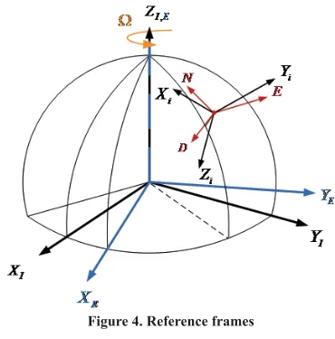
Before starting the modeling process, a useful reference frame named auxiliary inertial frame (X_i,Y_i,Z_i), should !!! vectors representations. The auxiliary inertial frame is simply an inertial frame where in which its origin and axes orientation coincide with those of the navigation frame (N,E,D) at navigation starting time, Figure 4.

Figure 4. Reference frames

A. Gimbals angles pickoffs modeling

coordinates is given as:

/ / /

p p p g

p i p g g

C

g i

Z

G

Z

G

Z

G

(1)

where

/

g g i

Z

G

is the angular velocity vector of the gyro frame !! coordinates,

/

p p g

Z

G

is the angular velocity vector of the platform !! -!!! +

/

g i

ZG !=@_?

represents the angular velocity at which the gyros are commanded to process relative to auxiliary inertial frame. CG_g The second represents gyro frame angular velocity relative to auxiliary inertial frame due to all gyro imperfections and is commonly referred to as gyro

drift. DG_g& "!

gyros are uncommanded and CGg G0. Subsequently,

the, and equation (1) becomes

/

p p g

p i g

C D

g

Z

G

G

(2)

On the other hand, using consequent rotations of yaw, pitch, and roll gimbals, p _/

p i

Z

G can be written as follows

/ / / / /

p p p p p

p i p PG PG RG RG B B i

Z

G

Z

G

Z

G

Z

G

Z

G

(3)

Where B, RG and PG refer to IMU body, roll, and pitch gimbals, respectively.

Assuming that the IMU is rigidly mounted to on a

stat-of the rotating earth and equation (3) can be written in the following form

^

`

/ /

/ / /

p p p

p i p PG PG

PG PG RG RG B n

PG RG RG RG B B n n i

C

C

C C

Z

Z

Z

Z

Z

G

G

G

G

G

(4)

Using equations (2) and (4), time rates of change of IMU gimbals pickoffs angles are given by

{

[

]

[

]}

z z y y x x y x x gx gy

x L y

L z y

L x L

C D

S D

S

C

S

C

S

C

C

S

S

C

C

T T T T T T T T T

T

K

K

K

K

:

:

:

:

(5)

^

x x

`

^

x x

`

z z

y L z y L x

gx gy

C

C

S

S

C

S

S D

C D

T T T T

T T

T

:

K

K

:

K

(6)

^

`

{

{

}

{

}}

y

y x x

x x

z gz L L y x

L z y

L x

D

S

C

S

C

C

S

C

S

S

C

T

T T T

T T

T

K

T

K

K

K

:

:

:

:

(7) Where

D_g: Gyros drift vector

$ : IMU case installation errors z|~

L : Geographic latitude

Gimbals pickoffs angles %_x, %_y, and %_zcan be found by solving equations (5), (6), and (7).

B. IMU velocity modeling

!! frame is given by

>

0

0

@

T

n s

f

G

g

₍₈₎

The time derivative of imperfect IMU velocity vector !!

a

a a a

a s a

V

G

K

f

G

B

G

(9)

Where

B_a is aaccelerometers bias vector,.

K_a is 3x3 diagonal matrix of the actual accelerometers scale factors which differ from the nominal

acceler-ometers scale factor vector by

*-ometers scale factor error vector.

0

0

0

0

0

0

x x

a y y

z z

K

dK

K

K

dK

K

dK

ª

º

«

»

«

»

«

»

¬

¼

(10)

a

a a p PG RG B n a

a p PG RG B n s a

V

G

K

C

C

C

C C f

G

B

G

(11)

Using initial alignment error matrix to write equation (11) in the auxiliary inertial frame gives

i i p a

p a

i p a p PG RG B n a

p a a p PG RG B n s a

V

C C V

C C K

C

C

C

C C f

B

G

G

G

G

(12)

Expanding and simplifying equation (12), time deriv-ative components of imperfect IMU velocity vector co-!!

1 2 3

x z y

V

s

]

s

]

s

(13)

1 2 3

y z x

V

]

s

s

]

s

(14)

1 2 3

z y x

V

]

s

]

s

s

(15)

where

1 1

2 2

3 3

ax ax

ay ay

az az

s

K a

B

s

K a

B

s

K a

B

z x z y x

z x z y x

a g S S C S C a g C S S S C a gC C

T T T T T

T T T T T T T

]Initial alignment errors

IMU velocity components: V_x, V_y, and V_z, can be found by solving equations(13), (14), and (15).

C. Gimballed IMU SimMechanics model

%!!! groups: validation directly with the original system out-puts, comparisons with already provided outputs by other scholars and developing another model using a completely different method which may not be applica-ble on some systems.

% ! ! the lack of resources, but we are lucky because our sys-tem can be modeled in another way based on

kinemat-ic relations, using SimMechankinemat-ics library in MATLAB SIMULINK. Hence, a perfect (error-free) IMU model can be easily created.

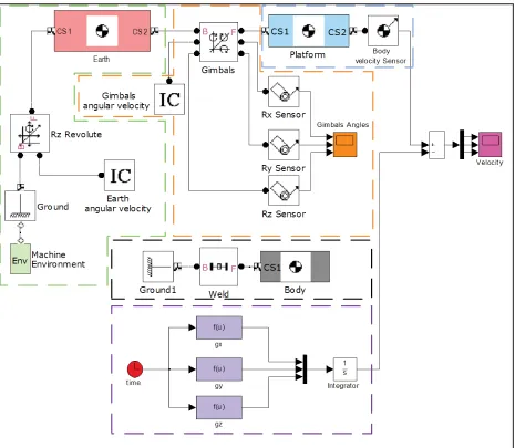
Figure 5 represents the developed model in MATLAB SIMULINK using SimMechanics library blocks, and as !!!!-tems as following:

 Earth frame: this subsystem simulates the earth movement relative to earth centered inertial frame

I-frame. In order to do this a spherical body with a !+€!!* !ZY@!! !" block.

 Gimbals: this subsystem is composed of gimbal joint which simulates IMU gimbals and three ‚|! rotation angles.

 ƒ | !

block which is a body located on the earth surface and connects it to gimbal joint, then adds a body velocity sensor to measure platform linear veloc-ity vector.

 Auxiliary inertial frame: at navigation start time, ZY@ !! do this a body block is added and connected to

I-frame using weld joint.

 Gravity vector components: SimMechanics soft-ware considers all forces, gravitational and !* comparison with our mathematical model will be meaningless, unless the gravitational force is ex-!!! where time-variant gravity vector components are integrated to be subtracted later from body veloc-ity sensor output.

3 IMU CALIBRATION METHODOLOGY

Since static IMU hardware error sources can be ! „ ! source to an accuracy, such that the navigational accu-racy achievable with the IMU, that would be limited only by non-compensable random disturbances.

Figure 5. IMU model using SimMechanics tools

Although, any navigation laboratory dealing with !…Y+ ! ! equipments, we prefer to reduce calibration equipments as much as possible for both decreasing external error sources and enhancing the cost-effectiveness. In addi-tion to the laboratory computer that leads the calibraaddi-tion process, only a precise tilting table used to align IMU !-duct our calibration process.

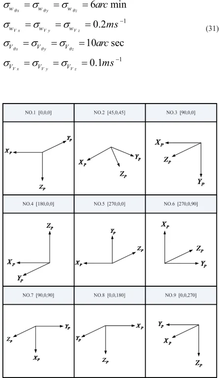
Given that the IMU case is aligned to the navigation frame, different relative platform-to-navigation frame angular orientations can be obtained by gimbal rota-tions, thus obviating any need to rotate the IMU case. These angular orientations are required for separation of the IMU error sources.

The preceding derivations of IMU output in the previ-ous section have resulted in a set of six general simul-taneous equations relating the six-system-level IMU measurable quantities to 15 error sources. Since a set of ! +-tions cannot be solved for 15 unknowns, a means func-tionally separating the error quantities had to be formu-lated. In view of the stochastic nature of the equations and IMU measurement noise, stochastic estimation of the error quantities would be the best solution possible.

the number of unknowns, accurate stochastic estimation of IMU error sources should be possible. The +-plished by angularly orientating the platform at various attitudes relative to the earth rate and gravity vectors by directly from the observation that the measurable IMU outputs are functions of both the IMU error sources and the components of earth rate and gravity vectors in the platform as well as inertial reference frames.

An off-line IMU calibration approach greatly facili-tates the development of data analysis computer pro-gram since it can be written in a higher order language, and is suitable for in lab calibration techniques.

Finally, total calibration time of few hours or less is recommended to allow aided-inertial navigation soft-ware tests to be conducted on the same days as the cal-ibration tests, and to preserve IMU work hours since they are limited.

Although many optimal stochastic estimation tech- +K-sidered to be the most applicable approach.

4 OPTIMAL ESTIMATION AND SMOOTHERS

A. EKF ALGORITHM

To write the system model in state space form we !!x, since we want to estimate IMU error parameters included in the derived set of differential equations, and the measurements are only IMU gimbals pickoffs angles and IMU velocities. Therefore, the only choice we have is a (21×1) vector as the following

, , , ,

, , , ,

, , , , , ,

x y z

x y z

ax ay az

gx gy gz

x y z

x y z

x y z

V

B

D

x

dK

T

K

]

ª

º

«

»

«

»

«

»

«

»

«

»

«

»

«

»

«

»

«

»

«

»

¬

¼

(16)

Therefore, system dynamics model can be written as follows:

, , ,

x

l x

:

L g

(17)

Where

l4$@‡@5!@Q

-ros, since x₇ to x₂₁ are constants.

To keep the implementation simple, the continu-"!+4@ˆ5!! a simple Euler integration scheme to give.

>

@ > @

> @

1

, , ,

, , , ,

x k

x k

T l x

L g

f

x k

L g T

:

:

(18)

Completing the system dynamics model by adding process noise we get the following

>

1

@

> @

, , , ,

> @

x k

f

x k

:

L g T

Bw k

(19)

Where

T is sampling time,.

f is a resultant (21×1) nonlinear vector of Euler inte-gration,.

w ~N

4JŠ54‹‡@5Œ"-ed, white noise,.

and B is (21×6) noise distribution matrix.

The measurements model is discrete and is given by

> @

> @ > @

y k

H x k

v k

(20)

Where

v~N(0,R) 4‹‡@5Œ"-ed, white noise,.

and H is (6×21) measurement distribution matrix.  ! system dynamics model since the measurements are in discrete-time form.

> @

,

i

ˆ

> @

k

j

f

A

i j

x k

x

w

w

(21)

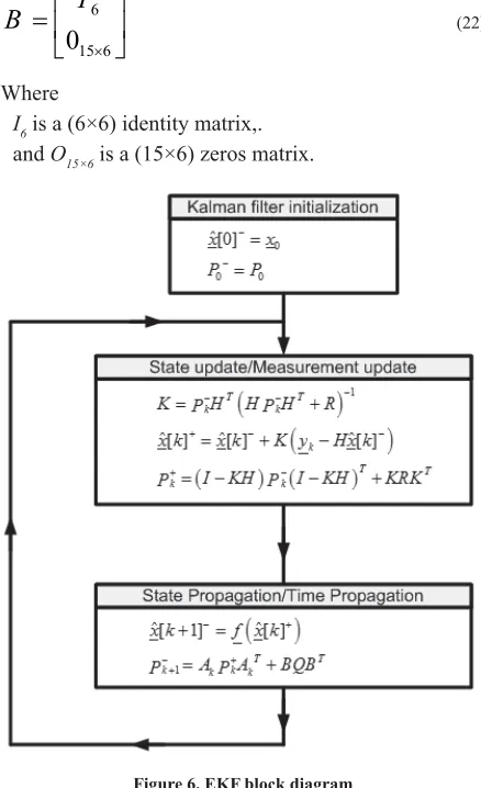
#!~!!K of study is shown in Figure 6.

velocity V measurement states, since IMU error param-!€!# elements.

The (21×6) noise distribution matrix B is illustrated +4$$5-ments that which are located in the rows correspond-ing to the gimbal angle % and velocity V measurements states. 6 15 6

0

I

B

u

ª

º

«

»

¬

¼

(22)

Where

I₆ is a (6×6) identity matrix,.

and O_15×64@Q‡‹5

Figure 6. EKF block diagram

The disturbance vector w is (6×1) input vector whose " white noise processes are assumed to be uncorrelated with each other resulting in the (6×6) system noise di-agonal matrix Q.

2 2 2 2 2 2

0 0 0 0 0

0 0

0 0 0

0

0 0 0 0

0 0 ₀ 0 0

0 0 0 0 0

0 0 0 0 ₀

w_x y z V x V y wV z w w w w Q T T T V V V V V V ª º « » « » « » « » « » « » « » « » « » ¬ ¼

Disp (23)

Where

&

w%x is %x system noise standard deviation.

The (6×21) measurement matrix H contains six non- !-sponding to the rows of the gimbal angle % and velocity

V measurement states.

H=[I₆ O_6×15] (24)

The measurement noise vector v is a (6×1) vector " These white noise processes are assumed to be uncor-related with each other resulting in the (6×6) measure-ment noise diagonal matrix R.

2 2 2 2 2 2

0 0 0 0 0

0 0

0 0 0

0

0 0 0 0

0 0 ₀ 0 0

0 0 0 0 0

0 0 0 0 ₀

x y z V x V y V z V V V V V V R T T T V V V V V V ª º « » « » « » « » « » « » « » « » « » ¬ ¼ (25) Where &

v%xis %x measurement noise standard deviation. The (21×21) covariance matrix P is initially a diago-nal matrix composed of the IMU error source variances. # "+! each time the platform frame is re-oriented since the variances of the velocity and gimbal angle measure-ment states having have increased during testing at a !!

B. Forward-Backward smoothing

To estimate the state x_m based on measurements from

k=1 to k=N, where N >m, forward-backward approach to smoothing obtains two estimates of x_m

-timate, x'mf !!!K

operates from k=1 to k=m. The second estimate, '_mb, is !K!

k=N to k=m. Then the forward-backward approach to smoothing combines the two estimates to form an opti-mal smoothed estimate '_m.

ˆ

ˆ

ˆ

f b

m f m b m

Where

K_f and K_b

Using both forward covariance matrix, P_f , and back-ward covariance matrix, P_b, that result from Kalman

K_f and K_b can be calculated as

follows

1

1

f b f b b f f b

K

P P

P

K

P

P

P

(27)

The inverse of (P_f+P_b ) always exists since both !=@Q? matrix of the forward-backward smoother is given by

_{1 1}

1

f b

P

P

P

(28)

K!+ should be written in reverse form

>

@

> @

>

@

> @

> @ > @

1 1

1 1 1

1

_{k k k}

1

k

x k

A

x k

A

B

w k

y k

H x k

v k

(29)

The inverse A-1

k-1 should always exist if it comes from

a real system. And the forward-backward smoothing al-gorithm for our case of study is shown in Figure 7.

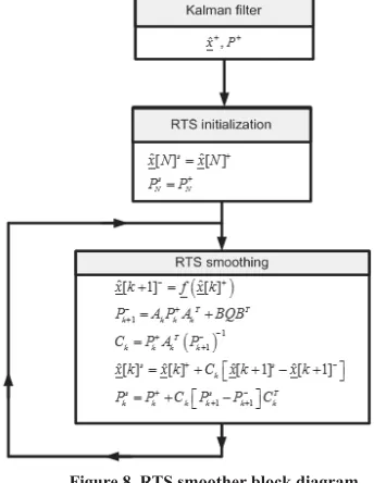
C. RTS smoother

One of the most common smoothers is that was pre-sented by Rauch, Tung, and Striebel, usually called the RTS smoother. RTS smoother is more computationally !"! do not need to directly compute the backward estimate or covariance in order to get the smoothed estimate or covariance [15].

Y ! K!…!-plementing the smoothing equations were presented in ' ” ! time with the following initial conditions.

> @

> @

ˆ

s

ˆ

s N N

x N

x N

P

P

(30)

Where • [N]s _{and P} N

s

are the smoothed state estimation and error covariance at the Nth _step.

Figure 7. Forward-backward smoother block diagram.

Figure 8. RTS smoother block diagram.

5 SIMULATION RESULTS

A. IMU Modeling and validation

Time rates of changes of IMU gimbals angles and time derivative of IMU velocity vector have been derived in previous sections. By solving theses differential equa-tions using Runge-Kutta integration algorithm, IMU gimbals angles and velocities can be obtained.

Y ! mathematical model could be compared with the per-fect IMU model developed in SimMechanics.

Figure 9 illustrates IMU gimbals angles and velocity simulation results for IMU at in test location case.

Figure 10 illustrates perfect IMU gimbals angles and velocity simulation results for IMU at test location case

Y%–_x returns to

MAT-LAB round process in[-180°,180°] range. These two !!

Figure 9. IMU output at test location (presented modeling).

Figure 10. IMU model validation at test location (SimMechanics)

B. IMU Calibration

Assume that we select a proper sample rate and data saving time, an important question will arise: “how ! ! ! -quence in the calibration process?”. The answer to this question is not obvious question, but we can say that IMU parameters number to be calibrated affects the at-titudes total number in a common sensegeneral wasy. As a result, selecting IMU calibration attitudes should be done by trial-and-error process until we reach to a !+

! ! ! -sponding gimbal angle rotations used in the implement-ed calibration process are illustratimplement-ed in Figure 11.

Considering nine IMU platform attitudes with data sample rate of T=30 sec and attitude period of atti-tude_time=10 min, total measurement time during the calibration procedure is will be 90 minutes and total measurement count is will equal 189 samples×6 IMU outputs.

Figure 12 shows EKF estimation, forward-backward and RTS smoothers results for only platform x-axis ac-celerometer bias.

Measurement noise and process noise are both gener-!##†˜!™*!| a pseudorandom, scalar value drawn from a normal dis-tribution with the mean of 0 and standard deviation of 1. To einsure the estimation results, more than few IMU data sets must be generated, then the calibration results for the IMU error parameters are averaged to get the

Considering the following noise standard deviation values:.

1

1

6

min

0.2

10

sec

0.1

x y z

V x V y V z

x y z

V x V y V z

w w w

w w w

V V V

V V V

arc

ms

arc

ms

T T T

T T T

V

V

V

V

V

V

V

V

V

V

V

V

(31)

Figure 12. x accelerometer bias

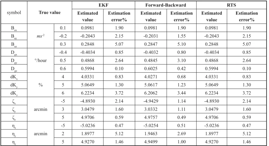
Table 1 lists EKF, forward-backward, and RTS esti-mation results considering last EKF estimated value of the IMU error parameters and averaging the smoothed values for both forward-backward and RTS smoothers for 100 simulation runs.

As explained, for full calibration process the measure-ments of nine IMU platform different attitudes should be applied serially to the calibration algorithms.

Table 2 illustrates how the IMU calibration error sources become separable as a function of the cumu-lative number of platform test attitudes employed. As sources could be estimated by the calibration algorithm. It means that up to this point, the measurements are not ! † !-ent attitudes, the calibration algorithms could estimate some of the other error sources of each test.

Both sets of velocity and gimbals pickoffs angle mea-surements were assumed to be available. The x’s indi-cates the earliest point at which the generated multiple sets of equations could be deterministically solved for a particular error source. All of the 15 IMU calibra-tion errors can be determined after 9 platform attitudes ‹ + !Q_+ are generated. Since only 15 equations should ideally be required, not all of the new equations generated are independent of previous ones.

6 CONCLUSION

In this paper, a mathematical model of 6-DOF gim-! "gim-!gim-! gim-!gim-!- !!-tail. 15 error sources are incorporated in the developed model including gyroscopes drift vector, accelerometers

bias vector, scale factor error vector, initial alignment imperfections and IMU case installation errors. Simula-tion results for three typical cases of non-rotating earth, equator case, and arbitrary location are presented. A validation technique using MATLAB SimMechanics tools is also presented and simulation results from both mathematical and SIMULINK models are compared to assure the correctness of mathematical model.

Assuming that all IMU error parameters are constants and using only system-level IMU outputs, simulation results show that employing 9 platform test attitudes is

!! K out an accurate estimation values. Also, simulation re-sults show that constant states are not smoothable and !! estimate of a constant state. However, there is no point in using smoothing for estimation of a constant state.

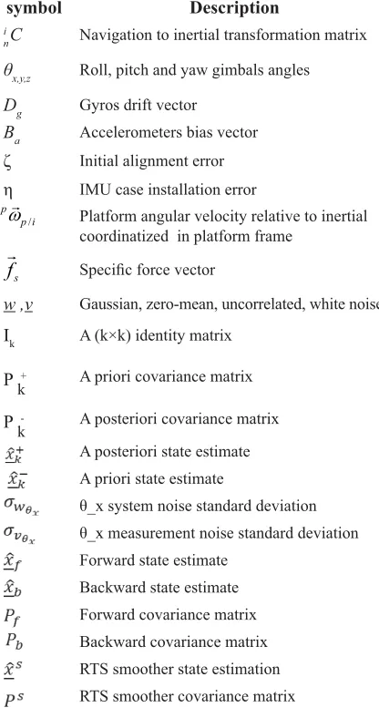
Glossary of variables

symbol Description

n

i _{C Navigation to inertial transformation matrix}

%_x,y,z Roll, pitch and yaw gimbals angles

D_g Gyros drift vector

B_a Accelerometers bias vector › Initial alignment error œ IMU case installation error

Platform angular velocity relative to inertial !!

Y

w ,v Œ"!

I_k A (k×k) identity matrix P

k

+ A priori covariance matrix P

k

- _{A posteriori covariance matrix}

A posteriori state estimate

A priori state estimate

–!!!

–!!!

Forward state estimate

Backward state estimate

Forward covariance matrix

Backward covariance matrix

RTS smoother state estimation

RTS smoother covariance matrix

/

p p i

Z

G

s

References

1. Jekeli C., Inertial Navigation System Geodetic, Walter de Gruyter GmbH & Co. KG, 2001.

2. Britting K.R., Inertial Navigation Systems Analy-sis, John Wiley & Sons, 1971.

3. K # % % # and Laboratory Test Results of a KALMAN Filter System-Level IMU Calibration Technique, Techni-cal Report AFAL-TR-77-75, June 1977.

4. Syed Z., Aggarwal P., Niu X., Goodall C. and El-Sheimy N., A New Multi-Position Calibration Method for MEMS Inertial Navigation Systems,

Measurement Sience and Technology, 18, 1897-1907, 2007.

5. Aggarwal P., Syed Z., Niu X. and El-Sheimy N., A Standard Testing and Calibration for Low Cost MEMS Inertial Sensors and Units, Journal of Nav-igation, 611, 323-336, 2008.

6. Shin E.H. and El-Sheimy N., A New Calibration

Attitude B_ax B_ay B D_gx D_gy D dK_x dK_y dK ›_x ›_y › œ_x œ_y œ 1

2 3 4

5 x x x

6 x x x x

7 x x x

8 x x x

9 x x

Table 2. separation of IMU calibration parameters symbol True value

EKF Forward-Backward RTS

Estimated value

Estimation error%

Estimated value

Estimation error%

Estimated value

Estimation error% B_ax

ms-2

0.1 0.0981 1.90 0.0981 1.90 0.0981 1.90

B_ay -0.2 -0.2043 2.15 -0.2031 1.55 -0.2043 2.15

B 0.3 0.2848 5.07 0.2847 5.10 0.2848 5.07

Dgx

°/hour

-0.4 -0.4034 0.85 -0.4032 0.80 -0.4034 0.85

D_gy 0.5 0.4868 2.64 0.4845 3.10 0.4868 2.64

D 0.6 0.5994 0.10 0.6025 0.42 0.5994 0.10

dKx

%

4 4.0331 0.83 4.0271 0.68 4.0331 0.83

dK_y 5 5.0649 1.30 5.0617 1.23 5.0649 1.30

dK 6 6.2234 3.72 6.2062 3.44 6.2234 3.72

›x

arcmin

-5 -4.8930 2.14 -4.9429 1.14 -4.8930 2.14

›_y 3 3.0479 1.60 3.0332 1.11 3.0479 1.60

› 5 4.9706 0.59 4.9757 0.49 4.9706 0.59

œx

arcmin

-5 -5.0236 0.47 -5.0254 0.51 -5.0236 0.47

œ_y 2 1.8977 5.12 1.9463 2.69 1.8977 5.12

œ 5 4.9270 1.46 4.9499 1.00 4.9270 1.46

Method for Strapdown Inertial Navigation Sys-tems, Z. Vermess, 127-10, 2002.

7. Fu L., Zhu Y., Wang L. and Wang X., A D-optimal Multi-position Calibration Method for Dynamical-ly Tuned Gyroscopes, ELSEVIER, 2010.

8. Wang X. and Shen G., A Fast and Accurate Initial Alignment Method for Strapdown Inertial Naviga-tion System on StaNaviga-tionary Base, Journal of Control Theory and Applications, vol. 3, no. 2, pp. 145-149, May 2005.

9. Wang X., Fast Alignment and Calibration Algo-rithms for Inertial Navigation System, Aerospace science and technology, vol. 13, no. 4-5, pp. 204-209, June-July 2009.

10. Hu C.H, Zheng J.F, Li J and Luo G.C, Rapid Self-Calibration for Small Gesture Inertial Plat-form before Launch, Journal of Chinese Inertial Technology, vol.3, 2007.

11. Yang L., Rapid Auto-Calibration for the Errors of Inertial Platform, Journal of Chinese Inertial Tech-nology, vol.4, 2000.

12. Shin Y.J. and Kim C.J., Fast Calibration Tech-nique for a Gimballed Inertial Navigation System, ICAS2002 CONGRESS, 2002.

13. Panahandeh G., Skog I. and Jansson M., Calibra-tion of the Accelerometer Triad of an Inertial Mea-surement Unit, Maximum Likelihood Estimation and Cramér-Rao Bound, IPIN International Con-ference @Q"@ˆ Y $J@J ¤ Y-land, 2010.

14. &Y!#!!Y-tion of Moving system, Ya Mahdi Publica&Y!#!!Y-tion, Teh-ran, ITeh-ran, 2010, (in Persian).

15. Simon D., Optimal State Estimation: Kalman, .A, and Nonlinear Approaches, John Wiley & Sons, 2006.