________________
*Corresponding author Received May 24, 2015
641
Available online at http://scik.org
J. Math. Comput. Sci. 6 (2016), No. 4, 641-652
ISSN: 1927-5307
ON SOME SLOPE-LIMITER METHODS FOR THE LINEAR ADVECTION
EQUATION
T. ABOIYAR1 AND B.V. IYORTER2,*
1Department of Mathematics/Statistics/Computer Science, University of Agriculture, Makurdi, Nigeria. 2Department of Mathematics and Computer Science, University of Mkar, Mkar, Nigeria
Copyright © 2016 T. Aboiyar and B.V. Iyorter. This is an open access article distributed under the Creative Commons Attribution License, which permits unrestricted use, distribution, and reproduction in any medium, provided the original work is properly cited.
Abstract: In this paper, we propose two slope-limiter methods for solving hyperbolic conservation laws. The methods are developed through flux formulation with piecewise linear construction and applied to solve the Linear Advection Equation using two initial conditions. The results which were compared with those of the Lax-Wendroff method, and the minmod method demonstrate the accuracy of the proposed methods.
Keywords: slope-limiter method; linear advection equation. 2010 AMS Subject Classification: 65N08.
INTRODUCTION
Conservation laws arise in many models in science and engineering. They are applied in fluid
and gas dynamics, relativity theory, quantum mechanics, aerodynamics, meteorology and
astrophysics (Eymard et al, 2003). Numerical methods for solving conservation laws include the finite difference method, finite element method and finite volume method. The finite volume
method is now a popular choice for solving conservation laws because of its accuracy and ability
to handle complex geometries as well as good approximations of boundary conditions (LeVeque,
2004, Hu & Joseph, 1990, Grigoryan, 2010, Moroney, 2006).
According to LeVeque (2004), finite volume methods for solving hyperbolic conservation laws
include Fromm’s method, Beam-Warming method and Lax-Wendrroff method. These methods
generate good approximations for smooth solutions but fail near discontinuities – they generate
methods that use slope-limiters to avoid the spurious oscillations that occur with high order
spatial discretization schemes due to shocks, discontinuities or sharp changes in the solution
domain(Mazzia, 2010).
In this paper, we propose two slope-limiters for solving hyperbolic conservation laws and have
applied them to solve the Linear Advection Equation, a type of conservation law.
METHODS
Formulation of Finite Volume Methods for Conservation Laws (LeVeque, 2004).
Consider the flow of gas in a tube where properties of the gas such as density and velocity are
constant. If 𝑢(𝑥, 𝑡) and 𝑣(𝑥, 𝑡) are the density and velocity of the gas respectively, the rate of
change of mass in [𝑥1, 𝑥2] is given as
𝑑
𝑑𝑡∫ 𝑢(𝑥, 𝑡)𝑑𝑥
𝑥2
𝑥1
= 𝑢(𝑥1, 𝑡)𝑣(𝑥1, 𝑡) − 𝑢(𝑥2, 𝑡)𝑣(𝑥2, 𝑡) (1)
Equation (1) is the integral form of conservation laws. If
𝐶𝑖 = (𝑥𝑖−1 2⁄ , 𝑥𝑖+1 2⁄ )
denotes the 𝑖th grid cell, then from equation (1) we have that
𝑑
𝑑𝑡∫ 𝑢(𝑥, 𝑡)𝑑𝑥𝐶
𝑖
= 𝑓 (𝑢(𝑥𝑖−1 2⁄ , 𝑡)) − 𝑓 (𝑢(𝑥𝑖+1 2⁄ , 𝑡)) (2)
Integrating equation (2) in time from 𝑡𝑛 to 𝑡𝑛+1, rearranging and dividing by ∆𝑥 gives
1
∆𝑥∫ 𝑢(𝑥, 𝑡𝐶 𝑛+1)𝑑𝑥
𝑖
= 1
∆𝑥∫ 𝑢(𝑥, 𝑡𝐶 𝑛)𝑑𝑥
𝑖
− 1
∆𝑥[∫ 𝑓 (𝑢(𝑥𝑖+1 2⁄ , 𝑡)) 𝑑𝑡
𝑡𝑛+1
𝑡𝑛
− ∫ 𝑓 (𝑢(𝑥𝑖−1 2⁄ , 𝑡)) 𝑑𝑡 𝑡𝑛+1
𝑡𝑛
] (3)
This suggests numerical methods of the form
𝑢̅𝑖𝑛+1 = 𝑢̅𝑖𝑛− ∆𝑡
∆𝑥(𝐹𝑖+1 2⁄
𝑛 − 𝐹
𝑖−1 2𝑛 ⁄ ) (4)
where 𝐹𝑖−1 2𝑛 ⁄ is some approximation to the average flux along 𝑥 = 𝑥𝑖−1 2⁄ at 𝑡 = 𝑡𝑛 given as
𝐹𝑖−1 2𝑛 ⁄ ≈ 1
∆𝑡∫ 𝑓 (𝑢(𝑥𝑖−1 2⁄ , 𝑡)) 𝑑𝑡
𝑡𝑛+1
𝑡𝑛
.
Equation (4) is the general form of the finite volume methods.
For the linear advection equation
𝐹𝑖−1 2𝑛 ⁄ ≈ 1
∆𝑡∫ 𝑎𝑢̃
𝑛(𝑥
𝑖−1 2⁄ , 𝑡)𝑑𝑡 𝑡𝑛+1
𝑡𝑛
From the cell average 𝑢̅𝑖𝑛, we can construct a piecewise linear function of the form
𝑢̃𝑛(𝑥, 𝑡𝑛) = 𝑢̅𝑖𝑛+ 𝜎𝑖𝑛(𝑥 − 𝑥𝑖) for 𝑥𝑖−1 2⁄ ≤ 𝑥 ≤ 𝑥𝑖+1 2⁄ (5 )
where
𝑥𝑖 = 1
2(𝑥𝑖−1 2⁄ + 𝑥𝑖+1 2⁄ ) = 𝑥𝑖−1 2⁄ + 1 2∆𝑥. The expression for the flux 𝐹𝑖−1 2𝑛 ⁄ becomes
𝐹𝑖−1 2𝑛 ⁄ = 1
∆𝑡∫ 𝑎𝑢̃
𝑛(𝑥
𝑖−1 2⁄ , 𝑡)𝑑𝑡 𝑡𝑛+1 𝑡𝑛 = 1 ∆𝑡∫ 𝑎𝑢̃ 𝑛(𝑥
𝑖−1 2⁄ − 𝑎(𝑡 − 𝑡𝑛), 𝑡𝑛)𝑑𝑡 𝑡𝑛+1
𝑡𝑛
= 𝑎𝑢̅𝑖−1𝑛 +1
2𝑎(∆𝑥 − 𝑎∆𝑡)𝜎𝑖−1
𝑛 .
Similarly,
𝐹𝑖+1 2𝑛 ⁄ = 𝑎𝑢̅𝑖𝑛−1
2𝑎(∆𝑥 − 𝑎∆𝑡)𝜎𝑖
𝑛.
Using the expressions for 𝐹𝑖−1 2𝑛 ⁄ and 𝐹𝑖+1 2𝑛 ⁄ in (4) gives
𝑢̅𝑖𝑛+1 = 𝑢̅𝑖𝑛 −𝑎∆𝑡 ∆𝑥 (𝑢̅𝑖
𝑛− 𝑢̅ 𝑖−1𝑛 ) −
1 2
𝑎∆𝑡
∆𝑥 (∆𝑥 − 𝑎∆𝑡)(𝜎𝑖
𝑛− 𝜎
𝑖−1𝑛 ) (6)
where 𝜎𝑖𝑛 is the slope in the 𝑖th grid cell 𝐶𝑖.
The finite volume method (6) depends on the choice of slope. Choosing the downwind slope (7)
gives the Lax-Wendroff method.
𝜎𝑖𝑛 =𝑢̅𝑖+1
𝑛 − 𝑢̅ 𝑖 𝑛
∆𝑥 . (7) But this slope is defined based on the assumption that the solution is smooth. Near a
discontinuity there is no reason to believe that introducing this slope will improve the accuracy.
Slope Limiters
Slope limiters are defined with the aim of limiting the solution gradient to avoid oscillations.
Accuracy is therefore expected even at discontinuities. Example of an existing slope-limiter is
the minmod slope defined as
𝜎𝑖𝑛 = minmod (𝑢̅𝑖
𝑛− 𝑢̅ 𝑖−1 𝑛
∆𝑥 ,
𝑢̅𝑖+1𝑛 − 𝑢̅𝑖𝑛
∆𝑥 )
minmod(𝑎, 𝑏) = {
𝑎 if |𝑎| < |𝑏| and 𝑎𝑏 > 0
𝑏 if |𝑏| < |𝑎| and 𝑎𝑏 > 0
0 if 𝑎𝑏 ≤ 0 .
Proposed Slope Limiters
We propose two slope-limiters which we call ‘amod’ and ‘bmod’, defined as
amod: 𝜎𝑖𝑛 = 1 2(
𝑢̅𝑖+1𝑛 − 𝑢̅𝑖−1𝑛
2∆𝑥 ) + 2 (minmod ( 1 2(
𝑢̅𝑖+1𝑛 − 𝑢̅𝑖−1𝑛 2∆𝑥 ) , (
𝑢̅𝑖+1𝑛 − 𝑢̅𝑖𝑛 ∆𝑥 )) ).
bmod: 𝜎𝑖𝑛 = mean(V, K)
where
V = minmod (2 (𝑢̅𝑖+1
𝑛 − 𝑢̅ 𝑖𝑛
∆𝑥 ) , (
𝑢̅𝑖𝑛− 𝑢̅𝑖−1𝑛
∆𝑥 )),
K = minmod ((𝑢̅𝑖+1
𝑛 − 𝑢̅ 𝑖𝑛
∆𝑥 ) , 2 (
𝑢̅𝑖𝑛− 𝑢̅𝑖−1𝑛
∆𝑥 )),
and
mean (𝑎, 𝑏) =𝑎 + 𝑏 2 . NUMERICAL EXPERIMENTS
In this section, we will solve the linear advection equation (8) with unit velocity subject to two
initial conditions.
𝑢𝑡+ 𝑢𝑥 = 0, 𝑥 ∈ [−1, 1] (8)
Solutions are obtained using the Lax-Wendroff method, the minmod method and the proposed
methods. We will solve for 𝑇 = 2. On the graphs, the red thick line represents the exact solution
while the blue dotted line represents the approximate solution. The minimum and maximum
values of the solutions – a test of accuracy of the methods, are obtained and tabulated.
Example One
Solve Equation (8) subject to the initial condition
𝑢(𝑥, 0) = sin(2𝜋𝑥). (9)
This is a smooth solution and the results are thus, presented in terms of errors, and the errors are
Table 1: Errors in 2-norm obtained from Solution of Equation (8) subject to initial condition
(9) by the downwind slope, minmod, ‘amod’ and ‘bmod’ limiters.
𝑵
Downwind limiter
(Lax-Wendroff method)
Minmod limiter
(minmod method)
‘amod’ limiter (‘amod’ method)
bmod’ limiter (‘bmod’ method)
50 4.9754 × 10⁻² 5.0369 × 10⁻² 5.0337 × 10⁻² 5.0400 × 10⁻²
100 2.5069 × 10⁻² 2.5147 × 10⁻² 2.5148 × 10⁻² 2.5148 × 10⁻²
200 1.2558 × 10⁻² 1.2568 × 10⁻² 1.2568 × 10⁻² 1.2569 × 10⁻²
400 6.2822 × 10⁻³ 6.2834 × 10⁻³ 6.2834 × 10⁻³ 6.2834 × 10⁻³
800 3.1415 × 10⁻³ 3.1416 × 10⁻³ 3.1416 × 10⁻³ 3.1416 × 10⁻³
Example Two
Consider Equation (8) subject to the initial condition
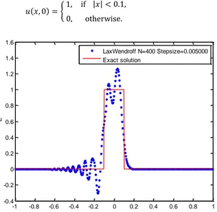
𝑢(𝑥, 0) = {1, if |𝑥| < 0.1,
0, otherwise. (10)
Fig. 1: Solution of Equation (8) subject to initial condition (10) using the Lax-Wendroff
method with 𝑁 = 400.
-1 -0.8 -0.6 -0.4 -0.2 0 0.2 0.4 0.6 0.8 1
-0.4 -0.2 0 0.2 0.4 0.6 0.8 1 1.2 1.4 1.6
x u
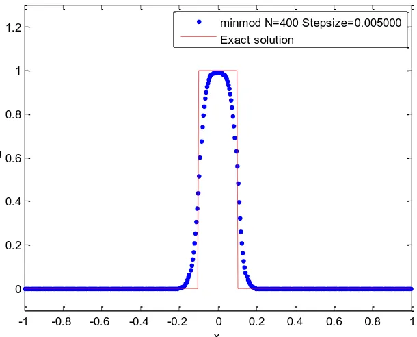
Fig. 2: Solution of Equation (8) subject to initial condition (10) using the minmod
method with 𝑁 = 400.
Fig. 3: Solution of Equation (8) subject to initial condition (10) using the ‘amod’ method
with 𝑁 = 400.
-1 -0.8 -0.6 -0.4 -0.2 0 0.2 0.4 0.6 0.8 1
0 0.2 0.4 0.6 0.8 1 1.2
x u
minmod N=400 Stepsize=0.005000 Exact solution
-1 -0.8 -0.6 -0.4 -0.2 0 0.2 0.4 0.6 0.8 1
0 0.2 0.4 0.6 0.8 1 1.2
x u
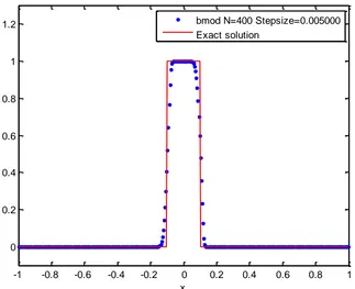
Fig. 4: Solution of Equation (8) subject to initial condition (10) using the ‘bmod’ method
with 𝑁 = 400.
Table 2: Minimum and Maximum values of the Exact Solution, and approximate solution
of Equation (8) subject to initial condition (10) by Lax-Wendroff, Minmod,
‘amod’ and ‘bmod’ methods with 𝑁 = 400.
Method Min(𝒖) Max(𝒖)
Exact 0.0000 1.0000
Lax-Wendroff −0.3053 1.2618
Minmod 0.0000 0.9927
‘amod’ −0.0095 1.0095
‘bmod’ 0.0000 1.0000
Example Three
Consider Equation (8) subject to the initial condition
-1 -0.8 -0.6 -0.4 -0.2 0 0.2 0.4 0.6 0.8 1
0 0.2 0.4 0.6 0.8 1 1.2
x u
𝑢(𝑥, 0) =
{
1
6𝐺(𝑥, 𝑧 − 𝛿) + 𝐺(𝑥, 𝑧 + 𝛿) + 4𝐺(𝑥, 𝑧) , − 0.8 ≤ 𝑥 ≤ −0.6
1, − 0.4 ≤ 𝑥 ≤ −0.2
1 − |10(𝑥 − 0.1)|, 0 ≤ 𝑥 ≤ 0.2
1
6𝐹(𝑥, 𝑎 − 𝛿) + 𝐹(𝑥, 𝑎 + 𝛿) + 4𝐹(𝑥, 𝑎), 0.4 ≤ 𝑥 ≤ 0.6
0, otherwise
(11)
where 𝐺(𝑥, 𝑧) = exp(−𝛽(𝑥 − 𝑧)2) , 𝐹(𝑥, 𝑎) = {max (1 − 𝛼2((𝑥 − 𝑧)2, 0}12. The constants are
taken as 𝑎 = 0.5, 𝑧 = −0.7, 𝛿 = 0.005, 𝛼 = 10, and 𝛽 = (log 2) 36𝛿⁄ 2.
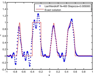
Fig. 5: Solution of Equation (8) subject to initial condition (11) using the Lax-Wendroff
method with 𝑁 = 400.
-1 -0.8 -0.6 -0.4 -0.2 0 0.2 0.4 0.6 0.8 1
-0.4 -0.2 0 0.2 0.4 0.6 0.8 1 1.2 1.4 1.6
x u
Fig. 6: Solution of Equation (8) subject to initial condition (11) using the minmod
method with 𝑁 = 400.
Fig. 7: Solution of Equation (8) subject to initial condition (11) using the ‘amod’ method
with 𝑁 = 400.
-1 -0.8 -0.6 -0.4 -0.2 0 0.2 0.4 0.6 0.8 1
0 0.2 0.4 0.6 0.8 1 1.2
x u
minmod N=400 Stepsize=0.005000 Exact solution
-1 -0.8 -0.6 -0.4 -0.2 0 0.2 0.4 0.6 0.8 1
0 0.2 0.4 0.6 0.8 1 1.2
x u
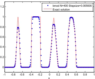
Fig. 8: Solution of Equation (8) subject to initial condition (11) using the ‘bmod’ method
with 𝑁 = 400.
Table 3: Minimum and Maximum values of the Exact Solution, and approximate solution
of Equation (8) subject to initial condition (11) by Lax-Wendroff, Minmod,
‘amod’ and ‘bmod’ methods with 𝑁 = 400.
Method Min(𝒖) Max(𝒖)
Exact 0.0000 1.0000
Lax-Wendroff −0.3053 1.2618
Minmod 0.0000 0.9927
‘amod’ −0.0095 1.0095
‘bmod’ 0.0000 1.0000
-1 -0.8 -0.6 -0.4 -0.2 0 0.2 0.4 0.6 0.8 1
0 0.2 0.4 0.6 0.8 1 1.2
x u
DISCUSSION
Table 1 shows result of Equation (8) subject to initial condition (9). The obtained result shows
that the Lax-Wendroff method produced errors slightly less than the other methods hence, more
accurate. This shows the efficiency of the Lax-Wendroff method for smooth solutions. Figures 1
and 5 are solutions obtained using the Lax-Wendroff method. The results clearly demonstrate the
deficiency of finite volume methods that are not slope-limiter methods – near discontinuities
they generate oscillations. Figures 2 and 6 are solutions by the existing slope-limiter method, the
minmod method. Here, no oscillations are generated rather; the discontinuities that arose in the
solution are resolved. However, the solution suffers from numerical diffusion. Figures 3 and 7
are solutions by the proposed ‘amod’ method. This method produced good results and resolves
the discontinuities that arose in the solution. Nevertheless, slight oscillations are observed near
discontinuities. Figures 4 and 8 are solutions by the proposed ‘bmod’ method. Results produced
here are accurate and discontinuities that arose in the solution are properly resolved, even better
than the minmod method. No case of oscillation is recorded even at discontinuities.
The results discussed above are evident in Tables 2 and 3. The tables record the minimum and
maximum values of the solutions to demonstrate the accuracy of the methods. They show which
methods produce oscillations and which do not.
CONCLUSION
The proposed methods produced good results compared to the existing ones. The methods should
therefore be used as alternatives to the existing ones. In general, slope-limiter methods produced
better results than finite volume methods that are not limiter methods, therefore,
slope-limiter methods should be applied to solve the linear advection equation in particular, and
conservation laws in general.
Conflict of Interests
The authors declare that there is no conflict of interests.
REFERENCES
[2] Grigoryan, V. Partial Differential Equations. Lecture Notes. Department of Mathematics, University of California, Santa Barbara (2010).
[3] Hu, H. H. & Joseph, D. D. Benchmark Flow around a Confined Cylinder. Journal of Non-Newtonian Fluid
Mechanics. 37(1990): 347 – 377.
[4] LeVeque, R. J. Finite Volume Methods for Hyperbolic Problems. 2nd edition, New York, Cambridge
University Press. (2004) 580.
[5] Mazzia, A. Numerical Methods for the Solution of Hyperbolic Conservation Laws. Science Applicate, via Belzoni, Italy. (2010)