Study of a Flowerlike Deployable Structure

(1)

0 INTRODUCTIONS

Umbrellas, fans and tents, which have similar features in common allowing them to be folded and deployed, are widely used in daily life [1] and [2]. When they are folded, their volumes are small and they can be stored and carried easily. When they are deployed, large surface areas or volumes are obtained. These kinds of structures are called deployable structures [3]. These characteristics of deployable structures have been used to solve difficult problems in space exploration equipment, such as satellite antennas and solar arrays [4] and [5]. Under working conditions, space exploration equipment is required to have large surface areas. However when they are put into launchers, their volumes have to be small. Therefore, deployable structures have been researched and applied in the area of spaceflight, and due to this important application, deployable structures have undergone rapid development [6].

In this paper, one kind of flowerlike deployable structure was studied. The deployable structure is a mechanism that is deployed to form a circle plane. Its shape is similar to a kind of flower whose petals surround the flower core. The movement of the mechanism is such that its petals rotate away from the fixed flower core to a state of complete deployment. Moreover, movements of the petals all are same and synchronous. According to the above requirements, we designed a flowerlike deployable structure as described below.

1 DETERMINING THE NUMBER OF PETALS

Because the flowerlike deployable structure is required to form a circle plane after its complete

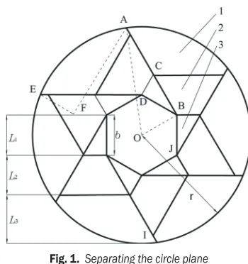
deployment, the shapes of its petals and rigid planes (in Fig. 1, surfaces 1, 2 and 3 refer to rigid planes, and the rigid planes compose a petal) on every petal can be obtained by separating the circle plane. The shapes of the petals and rigid planes refer to the reference [7]. When the deployable structure is folded, its petals are needed to surround the central member. So the its central member is a regular polygon and the shapes of all petals of the mechanism should be the same. The circle plane is separated as shown in Fig. 1.

Fig. 1. Separating the circle plane

When the deployable structure is folded, its section shape is shown as in Fig. 2a. The thickness of the rigid planes can be neglected, because the length of the diameter of the circle plane formed after deploying the mechanism completely is three magnitudes larger than the thickness of the rigid planes. L1 and L2 (shown in Fig. 1) must be equal to the side length of the central regular polygon b, which simplifies the folded deployable structure as shown in Fig. 2b. The

Study of a Flowerlike Deployable Structure

Luo, A. – Liu, H. – Li, C. – Wang, Y. Ani Luo – Heping Liu – Cheng Li – Yongfan Wang

College of Mechanical and Electrical Engineering, Harbin Engineering University, China

A deployable structure is a kind of mechanism that can be folded and deployed automatically. It is able to form required shape or curved surface after deployment. In this paper, a flowerlike deployable structure, which forms a circle plane after deployment, was studied. First, the required circle plane was decomposed to determine the shapes of the members. Then the relation expressions were set up, which include the structural dimensions of the members and how to calculate the volume of the mechanism in the folded state. The number of the petals was optimized with the aim of minimizing the volume of the structure in its folded state. In order to determine the connecting forms among the petals and in one petal, the degrees of freedom of the mechanism were studied. On the basis of these analysis results, the flowerlike deployable structure was designed in detail. Using mechanical topology analysis, the mechanism was simplified. Based on the screw theory, the vector form output matrix of the mechanism was built. After analysing its mobility, the driving inputs positions were obtained. Finally, a virtual prototype technology was used to verify the feasibility of the design.

(2)

relation of the structural dimensions of the mechanism is analysed in order to obtain the folded shape of the deployable structure shown in Fig. 2. The relationship is shown by the following

p b

s r b s

-cos / sin

,

1

180 ₂ 180

1

2 2

(

)

( )

−

(

( )

)

≤ (1)

where p is number of rigid planes on a petal of the deployable structure, b side length of the regular polygon, r radius of the circle plane formed after deployment of the mechanism and s number of its petals.

a)

b)

Fig. 2. Simplified section of the deployable structure in the folded state

The section shape of the deployable structure in folded state is simplified as shown in Fig. 2b. In the Fig 2b, OJ is the distance from a tip of the central polygon to its center and OI is the distance from the point remotest to the center to the central point. The angle of OI and OJ is (180°/s), and the structural dimensions of the deployable structure are:

IO= r − (p− )× × +r b ( p− )( p− )b + b _° s

2 2 2

2

2 1 2 1 2 3

4 ₄_sin 180 . (2)

The length AF shown in Fig. 1 is the maximum axial height of the mechanism in the folded state. With an analysis of the geometrical dimensions, AF can be solved as:

AF= 4sin2180°× 2− 2.

s r b (3)

Eq. (1) is transformed to get:

b r

p

s s

≤ −

(

)

°+ °

1

180 ₄ 1180

2

2 2

cos sin

. (4)

So, the maximum of b can be calculated from Eq. (4). The folded deployable structure can be put into a cylindrical case. The inner radius of the case is equal to the length of IO, and its height is equal to the length of AF. We let the volume of the deployable structure in the folded state equal that of the case. Therefore, the volume V of the deployable structure in the folded state is approximately solved as:

V r p r b

p p

b b

= ×

   ×

×

π 2

2 2

2

2 1

2 1 2 3

4 ₄ 180

4

sin s

ssin2180°_× 2₋ 2.

s r b (5)

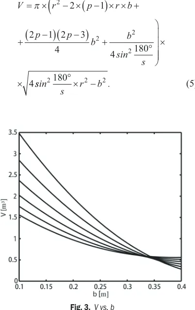
Fig. 3. V vs. b

(3)

3 shows the resulting V vs. b for the simulation. As shown in Fig. 3, V is inversely proportional to b. After further analysis, when p is equal to other constant, V is still inversely proportional to b..

V is the main characteristic of the deployable structure and is required to be minimized. With the aim of minimizing V, using the above result, s can be determined as shown below. Let r equal 1 m. When p equals 3, after calculating with Eq. (4), s, b and V are summarized in Table 1. When p is equal to other values, values of s, b and V are similar to those in Tab.1. Therefore, the conditions when p is equal to another value are omitted here.

From Table 1, it is known that when s is equal to 6, b is at its maximum value, and V is at its least. So s is determined finally to equal 6..

Table 1. s, maximum b and V

s Maximum of b [m] V [m3_]

3 0.25 0.581

4 0.34 0.552

5 0.395 0.495

6 0.397 0.463

7 0.391 0.514

8 0.385 0.56

2 CALCULATING DEGREES OF FREEDOM

The flowerlike deployable structure is a multibody system and has complicated movement. In order to reduce the output energy and mass of the driving members and control the mechanism more easily, it is necessary to minimize the degrees of freedom (DOF) of the mechanism. Because DOF of a closed mechanism chain is less than an open one, links are needed to connect neighbour petals to make the mechanism into several close mechanism chains. To make movement of the deployable structure less complicated, let number of the links only equal 1 or 2,

and the kinematic pairs connecting the links and petals only be a revolute pair or spherical pair.

DOF of the space mechanism can be solved with the equation:

F n ui

i j =

(

−

)

−

=

∑

6 1

1 , (6)

where n is a number of members of the mechanism, j a number of its kinematic pairs, ui a number of

constraints of the i kinematic pair [8] to [10].

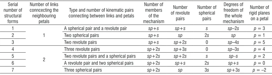
Let F be equal to s, and Eq. 6 is used to calculate the DOF of the flowerlike deployable structure with different connecting forms between the petals. The number of members and kinematic pairs and resulting DOF are summarized in Table 2.

Based on Table 2, the numbers of connecting links, kinematic pairs and the type of the kinematic pairs have a direct influence on p. In the 2nd_structural form, the number of members is too little so that ratio of volumes of the deployable structure in folding and deploying states is too large, which doesn’t fit requirement of the deployable structure. There are too many kinematic pairs in the 5th_{structure, and its} movement is complicated, which makes it difficult to control. The 6th_{and 7}th_{structure forms are obviously} impossible. So only the 1st_{, 3}rd_{and 4}th_{structure are} feasible. In the three feasible structures, the 1st structure has the least members, so it is adopted here.

3 TOPOLOGY ANALYSIS OF THE MECHANISM

Using the results of the above analysis, we designed a flowerlike deployable structure. A virtual prototype of the mechanism is shown in Fig. 4. It is composed of a hexagonal central plane and six petals. Each petal has three rigid planes, including a root rigid plane, middle rigid plane, and top rigid plane as shown in Fig. 4. The root rigid plane is a right-angled triangle. The surface of the middle rigid plane is trapezium. The top rigid Table 2. The number of members and DOF

Serial number of

structural forms

Number of links conncecting the neighbouring

petals

Type and number of kinematic pairs connecting between links and petals

Number of members

of the mechanism

Number of revolute

pairs

Number of spherical

pairs

Degrees of freedom of the whole mechanism

Number of rigid planes on a petal

1

A spherical pair and a revolute pair sp+s sp+s s sp–2s p = 3

2 Two spherical pairs sp+s sp 2s sp p = 1

3 Two revolute pairs sp+s sp+2s 0 sp–4s p = 5

4

2

Three revolute pairs sp+2s sp+3s 0 sp–3s p = 4

5 Two revolute pairs and a spherical pairs sp+2s sp+2s s sp–s p = 2

6 A revolute pair and two spherical pairs sp+2s sp+s 2s sp+s p = 0

(4)

plane has an amorphous formation. The rigid planes and the central hexagon plane are connected to each other via revolute pairs. A bar connects the two top rigid planes on the neighbouring petals together. There are a revolute pair on an end of the bar and a spherical pair on its other end.

Using mechanical topology analysis, we can simplify the mechanism and the result is shown in Fig. 5. The meanings of the below symbols, figures and terms can be found in reference [11].

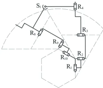
As shown in Fig. 5, the mechanism is composed of several close mechanism chains. In order to analyse the mechanism further, one must decompose the mechanism into several minimum close mechanism chains (the minimum close mechanism chains are called simply SLC). Because the mechanism is symmetrical, it can be decomposed into six identical SLC as shown in Fig. 6. The composition of the SLC can be expressed as:

SLC{–R1⊥R2 // R3⊥R4 – S1 – R8 // R9⊥R10–}, where Ri denotes the ith revolute pair and sj denotes

the jth_{spherical pair. In Fig. 6, the bar between R}₁_and R10 is cut and the spherical pair S1 can be substituted with three revolute pairs.

Fig. 4. The flowerlike deployable mechanism

Fig. 5. The flowerlike deployable structure after simplified

Fig. 6. A close mechanism chain (SLC)

The SLC is changed into an open mechanism chain (SOC) as shown in Fig. 7. The composition of the SOC can be expressed as:

SOC

{

−R1⊥R2/ /R3⊥R4⊥R5−R6−R7/ /R8/ /R9⊥R10−

}

.

Fig. 7. The open mechanism chain (SOC)

The below analysis will be carried out using Descartes coordinates. Using screw theory, we make a list of the independent outputs of the output eigenmatrix of every kinematic pair in turn, and these are then added together to get the vector form of the output matrix of the SOC as:

MS t

r R

t

r R

t R

r R

=   



   +



  



   +

⊥ 0

1 1 ₁

0

1

2 ₂

1 3 1

2

(/ / ) (/ / )

( )

(/ / / // )

(/ / ) (/ / )

R

t

r R

}



  



   +

+

_{

⊥

_}

  



   =

t R

r R

t R

r R

( )

(/ / )

( )

(/ / ) tt

r _S

3

3 

  



 

 . (6)

(5)

lines always intersect at one point and the outputs of the two revolute pairs are independent of each other. The axis line of R3 is parallel to R2, so rotation of R3 is independent relatively of R1 and R2. Therefore the revolute pair R3 produces a dependent translation. Rotation of R4 is not relative to R1 ~ R3, so its rotating output is independent. Rotating outputs of R5 and R6 have a relationship with the above revolute pairs and they will produce two independent translation outputs. Because there are six independent outputs, all outputs of R7 ~ R10 are dependent.

Independent rotations of the output matrix MS of the SOC are r1_{(// R}₁_{), r}1_{(// R}₂_{) and r}1_{(// R}₄_{), so} the number ξSR of its independent rotation outputs is

3. Independent translation outputs of the matrix are t1₍⊥_R₃_{), t}1₍⊥_R₅_{) and t}1₍⊥_R₆_{), and the number ξ}_SR_of its independent translation outputs is 3 too. Therefore order ξ of the output matrix Ms can be calculated as:

ξ = ξS = ξSR + ξSP = 3 + 3 = 6. (7)

4 DETERMINING THE POSITION WHERE INPUTS ARE LOCATED

DOF of the mechanism can be calculated using the equation:

F

f

_i

i m

=

−

=

∑

1

ξ

,

(8)

where F = DOF, fi = DOF of the ith kinematic pair and

m is a number of kinematic pairs in the mechanism. We use Eq. (8) to solve for DOF of the SLC as shown in Fig. 6. Because F > 0, namely ∑ fi＞ ξ，the

SOC (shown in Fig. 7) that the SLC is transformed to form is a redundance mechanism and its independent outputs can be completed only with R1 ~ R7. The SOC is simplified to get another SOC only composed of R1 ~ R7. The DOF of the SOC is solved as:

F

f

_i

i

=

− = − =

=

∑

1 7

7 6 1

ξ

.

(9)

The DOF result indicates that the SLC as shown in Fig. 6 only needs an input. Because R8 ~ R10 and R1 ~ R7 lie on different petals, in order to reduce movement coupling among the petals, the input will be placed at any of R1 ~ R7. Because the flowerlike deployable structure is composed of six identical SLC, only 6 inputs are required to control the mechanism completely.

The position of the input will be determined below. Before the analysis is carried out, it is estimated whether there are passive kinematic pairs in the mechanism shown in Fig. 7. After rigidizing R8 ~ R10, the composition of the SOC can be expressed as:

SOC*

1 2 3 4 5 6 7

− ⊥ ⊥ ⊥ − − −

{

R R / /R R R R R

}

.

Fig. 8. The open mechanism chain after rigidizing R1

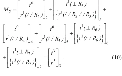
Then R1 is rigidized and the SOC is changed as shown in Fig. 8. We then list the independent outputs of output eigenmatrix of every kinematic pair in turn, and further obtain the vector form of the output matrix of the SOC shown in Fig. 8 as:

M_S t

r R

t R

        =         6 1 7 1 7 7 3 3 t R r R t r _S ( )

(/ / ) . (10)

The order of the Ms is calculated as:

ξ1* = ξS = ξSR + ξSP = 3 + 3 = 6.

The order of the SOC is same as in Fig. 7. The analysis method in reference [2] confirms that R1 is not a passive kinematic pair and that input can be located there.

The above analysis method is used further to determine whether R2 ~ R7 are passive kinematic pairs, and the result is summarized in Table 3.

(6)

Because R5, R6 and R7 are used to substitute for the spherical pair, inputs are not able to be located there. So inputs only are at R1 ~ R4. In the whole structure shown in Fig. 5, R1 ~ R3 in a SLC are expressed as R8 ~ R10 in the one next to it. If an input is placed at either R1, R2 or R3, it will influence movements of the two SLC, which makes movement analysis and control of the mechanism complicated. Because R4 only belongs to the SLC of the whole mechanism, and can not influence movements of other SLC, the input should be located at R4.

5 SIMULATION CHECK

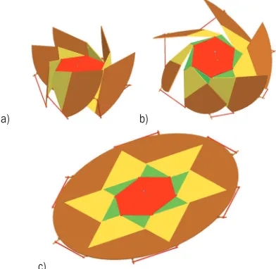
By analysing the results of the input position, we can set the virtual prototype of the flowerlike deployable structure and further simulate it. The movement of the inputs is designed to coincide with the sine law. From the boundary conditions of the movement of the mechanism, the movement equation of the inputs can be solved as:

θ =18 5. sin×

(

π×t/8 0 23+ .

)

.

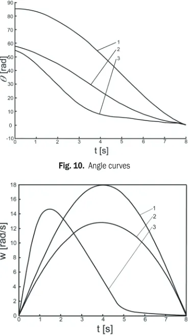
The virtual prototype of the flowerlike deployable structure moves from the folding state to deploying state as shown in Fig. 9, which proves that the flowerlike deployable structure can be folded and deployed automatically and that the design scheme is reasonable. Let θ1 equal the angle of rigid plane 3 and the central polygon in Fig. 1, θ2 be equal to the angle of rigid plane 2 and rigid plane 3, and θ3 equal the angle of rigid plane 1 and rigid plane 2. Figs. 10 and 11 show the resulting θi and ωi (i = 1, 2, 3) vs. time for

the simulation. As shown in Fig. 10, the rigid planes can rotate continuously to the desired positions. In Fig. 11, the angular velocities change continuously. The

beginning and end points of the curves are all 0, and there are no sudden changes in acceleration. So, there are no impulsions and vibrations in the movement of the mechanism.

a) b)

c)

Fig. 9. Movement of the flowerlike deployable structure

6 CONCLUSION

A deployable structure is a kind of mechanism that is deployed completely to form the desired surface or spatial structure. In this paper, a design method of for such a deployable structure is depicted. After analysis of the shapes of the mechanism in folding and deploying states, its volume in the folded state is solved and its number of petals is further determined. In calculating DOF, we select the structure connecting the petals and the number of the rigid planes. Using mechanical topology analysis and the screw theory,

Table 3. Determination of passive kinematic pairs Rigidized

6 No Yes

(7)

the position of the inputs is determined. From the analysis in this paper, the below conclusions are obtained:

(1) Because the volume of the deployable space structure in the folded state must be reduced, requiring that the structural dimensions of the mechanism be optimized with the aim of obtaining the minimum volume is reasonable. This has been verified in the paper;

(2) In order to make control of the mechanism easier, it is necessary to reduce the number of inputs into the mechanism, namely DOF. Therefore, the number of elements and type of kinematic pair in the mechanism can be determined via analysis of its DOF;

(3) Screw theory and mechanical topology analysis are combined, and thus the positions of the inputs can be determined correctly. This was also verified.

These methods have been used in this paper, and a feasible deployable structure has been obtained. Therefore, the methods can be applied in the design of this kind of deployable structure.

Fig. 10. Angle curves

Fig. 11. Angular velocity curves

7 ACKNOWLEDGMENT

This work was supported in member by the Special Fund from the Central Collegiate Basic Scientific Research Bursary (HEUCF110703) and the Heilongjiang Postdoctoral Science Foundation (323630297).

8 REFERENCES

[1] Puig, L., Barton, A., Rando, N. (2010). A review on large deployable structures for astrophysics missions. Acta Astronautica, vol. 67, no. 1-2, p. 12-26, DOI:10.1016/j.actaastro.2010.02.021.

[2] Brown, M.A. (2011). A deployable mast for solar sails in the range of 100-1000 m. Advances in Space Research, vol. 48, no. 11, p. 1747-1753, DOI:10.1016/j. asr.2011.01.014.

[3] Meguroa, A., Shintateb, K., Usuib, M., Tsujihatab, A. (2009). In-orbit deployment characteristics of large deployable antenna reflector onboard Engineering Test Satellite VIII. Acta Astronautica, vol. 65, no. 9-10, p. 1306-1316, DOI:10.1016/j.actaastro.2009.03.052. [4] Soykasap, Ö. (2009). Deployment analysis of

a self-deployable composite boom. Composite Structures, vol.89, p. 374-381, DOI:10.1016/j. compstruct.2008.08.012.

[5] Fazli, N., Abedian, A. (2011). Design of tensegrity structures for supporting deployable mesh antennas.

Scientia Iranica, vol. 18, no. 5, p. 1078-1086, DOI:10.1016/j.scient.2011.08.006.

[6] Fanchini, G., Gagliostro, D. (2011). The e-st@r CubeSat: Antennas system. Acta Astronautica, vol. 69, no.11-12, p. 1089-1095, DOI:10.1016/j. actaastro.2011.06.009.

[7] Guest, S.D. (1994). Deployable structures: concepts and analysis. PhD thesis. The University of Cambridge, Cambridge.

[8] Hopkins, J.B., Culpepper, M.L. (2011). Synthesis of precision serial flexure systems using freedom and constraint topologies. Precision Engineering, vol. 35, no. 4, p. 638-649, DOI:10.1016/j. precisioneng.2011.04.006.

[9] Gallardo, J., Lesso, R., Rico, J.M., Alici, G. (2011). The kinematics of modular spatial hyper-redundant manipulators formed from RPS-type limbs. Robotics and Autonomous Systems, vol. 59, no. 1, p.12-21, DOI:10.1016/j.robot.2010.09.005.

[10] Yu, J., Li, S., Su, H.-J., Culpepper, M.L. (2011). Screw Theory Based Methodology for the Deterministic Type Synthesis of Flexure Mechanisms. Journal of Mechanisms and Robotics, vol. 3, no. 3, p. 1-14, DOI:10.1115/1.4004123.