A numerical investigation of a reaction-diffusion equation arises
from an ecological phenomenon
Parastoo Reihani Ardabili
Department of Mathematics, Payame Noor University, Tehran, Iran. E-mail: p [email protected]
Abstract This paper deals with the numerical solution of a class of reaction diffusion equations
arises from ecological phenomena. When two species are introduced into unoccu-pied habitat, they can spread across the environment as two travelling waves with the wave of the faster reproducer moving ahead of the slower.The mathematical modelling of invasions of species in more complex settings that include interactions between species may restricts to pairwise interactions. Three mathematical models of invasions of species in more complex settings that include interactions between species are introduced. For one of these models in general form a computational approach based on finite difference and RBF collocation method is established. To numerical solution first we discretize the proposed equations by using the forward difference rule for time derivatives and the well known Crank-Nicolson scheme for other terms between successive time levels. To verify the ability and robustness of the numerical approach, two test problems are investigated.
Keywords. Ecological phenomena, Reaction-diffusion, Invasion, RBF collocation, Finite differences method.
2010 Mathematics Subject Classification. 65M20, 65M70, 35K61.
1. Introduction
Today the development of mathematical models is of vital importance for under-standing and management of ecological processes. Identifying the complex relation-ships between ecological patterns and processes is a crucial task [1,2,3,4,7,8,11, 14, 19]. Qualitatively and quantitatively, mathematical models play a vital role in analysing ecological systems.
Many ecological phenomena may be modelled using apparently partial differential equations (PDE’s) involving space and possibly time. Using these models allows modellers to well understand the complicate phenomena and to incorporate both temporal and spatial processes simultaneously into equations governing population dynamics [1, 3, 4, 8]. It is becoming clear that the simplest models cannot capture the rich variety of dynamics observed in natural systems.
On the other hand the PDEs that are sufficiently realistic to be used in ecological models are usually very complex and difficult to solve [1,3,8].
Reaction-diffusion equations are widely used as models for spatial effects in ecol-ogy. They support three important types of ecological phenomena: the existence
Received: 7 July 2017 ; Accepted: 9 December 2017.
of a minimal patch size necessary to sustain a population, the propagation of wave-fronts corresponding to biological invasions, and the formation of spatial patterns in the distributions of populations in homogeneous environments [3, 8]. These models emphasize that simple organism movement can produce striking largescale patterns in homogeneous environments and that in heterogeneous environments, movement of multiple species can change the outcome of competition or predation [3,8].
The first formal mathematical attempts to model ecological invasions via reaction-diffusion equations were made by Skellam ([19]) who modelled the expansion of muskrat populations in Europe. His model of invading animals with diffusion move-ment and malthusian growth predicts that the area occupied by an invader will increase linearly with time [3, 8]. Reaction-diffusion invasion models exhibit more striking behavior when population growth is not exponential but instead is regulated by density-dependent mortality. These models produce travelling waves of invaders that spread out from their ”beachhead” at a constant velocity and shape. Travelling waves are a common feature of many reaction-diffusion models [4]. A final refinement in invasion theory involves the relaxation of restrictions on population growth func-tions, by the addition of an Allee effect whereby at low densities population growth is negative [8]. Models involving population growth with an Allee effect plus diffusive dispersal also produce travelling waves of invaders [1,3,8,19].
Some classes of reaction-diffusion equations may be analyzed by means of methods from the theory of partial differential equations and dynamical systems. But usually finding the exact solution of nonlinear PDEs is a complex task and in a lot of nonlinear PDE problems, one can not solve them analytically. In recent years considerable studies has been done in the numerical solution of nonlinear PDEs. The investigation of exact and numerical solutions for nonlinear partial differential equations (NLPDEs) plays an important role in the study of nonlinear physical phenomena. These solutions when they exist can help one to well understand the mechanism of the complicated physical phenomena and dynamical processes modelled by these nonlinear evolution equations. In this paper an approximate solution for a system of nonlinear reaction-diffusion models is presented using radial basis functions (RBF) collocation method of lines. Recently using the RBFs has drawn attention of many researchers in science and engineering as a truly meshless method for approximating the solutions of linear and nonlinear functional equations such as PDEs. Several works have been adopted in this field in the literature [5,6,9,10,12,13,15,16,17,20,21]. Numerical studies illustrates the advantages of using this mesh-less methods to solve initial and/or boundary value problems [13,16]. In comparison with the classical methods such as finite difference or finite element methods for solving PDE’s, the RBF methods do not depend on computational grids or meshes and are very simple to implement [10,13]. In addition RBF methods usually possess superior rate of convergence [9, 12, 21]. The large number of recent research works on mesh-less methods especially RBF collocation method for solving nonlinear PDE’s demonstrates the popularity that the methods have recently enjoyed.
This paper is organized as follows:
numerical procedure based on finite difference and RBF methods to solve this problem. In section 4 some test problems are considered and analyzed. Section 5 contains the conclusions.
2. Problem formulation
In this section we review three nonlinear reaction-diffusion models proposed in [8]. According to [8], when two species are introduced into unoccupied habitat, they can spread across the environment as two travelling waves with the wave of the faster reproducer moving ahead of the slower. The mathematical modelling of invasions of species in more complex settings that include interactions between species may restricts to pairwise interactions. A reasonable model for the spread of two competing species can derived as [8]
∂u ∂t =Du
∂2u
∂x2 + (ru−αuuu−αuvv)u,
∂v ∂t =Dv
∂2v
∂x2 + (rvαvvv−αvuu)v,
(2.1)
where u and v are the densities of the two species, Du and Dv are species-specific
diffusion rates,ru andrv are species-specific intrinsic rates of increase, and theα,s
represent interspecific and intraspecific competition coefficients.
On the other hand the Lotka-Volterra predator-prey models with diffusion are represent similar mathematical formulation to predator-prey interactions [8, 4]. An important class of these models may be derived as [8]
∂u ∂t =Du
∂2u
∂x2 +ru(1− u
K)−αuvuv,
∂v ∂t =Dv
∂2v
∂x2 −µv+αvuuv,
(2.2)
where µthe per capita mortality rate of predators in the absence of prey, αuv
rep-resents the rate at which predators consume prey, and αvu represents the rate at
which predators convert prey into new predators. It should be pointed out that if both predator and prey colonize an environment that is initially empty, their spread cannot be mathematically represented by a travelling wave and the spread in this case does form wave-like patterns [3,4,8]. But if the prey already exists uniformly across the environment and a predator is released, the situation is analogous to the spread of disease through susceptible hosts, and travelling waves of predator and prey will ensue [4,8].
For investigating the influence of patch size and geometry on the population dynam-ics of organisms living within habitat patches, the proposed models may be considered in a more general form named the cross-diffusion model as follows [8]
∂u ∂t =Du∂
2u
∂x2 +ru(1− u
K) +ν(u),
∂v ∂t =Dv
∂2v
∂x2 −µv+ω(u),
(2.3)
functions. This model describes organisms that avoid each other by increasing their dispersal rate in response to both conspecifics and nonconspecifics [8].
For more details about the physical interpretation of these models, we refer the readers to [1, 3, 8] and the references therein. In sequence we focus on finding the numerical solution for the model (2.1). Similar procedures can be developed for solving the equations (2.2) and (2.3).
3. Method of solution
3.1. Discretization of the main problem. In this section a numerical procedure is established for solving the equation (2.1). To this end first we consider this equation in more general form as an initial-boundary value problem as follows
∂u ∂t =Du
∂2u
∂x2 + (ru−αuuu−αuvv)u+F(x, t), (x, t)∈Ω, (3.1) ∂v
∂t =Dv ∂2v
∂x2 + (rvαvvv−αvuu)v+G(x, t), (x, t)∈Ω, (3.2)
u(x,0) =f(x), (3.3)
v(x,0) =g(x), (3.4)
c1(t)u(0, t) +c2(t)ux(0, t) =φ1(t), (3.5)
c3(t)u(1, t) +c4(t)ux(1, t) =ψ1(t), (3.6)
c5(t)v(0, t) +c6(t)vx(0, t) =φ2(t), (3.7)
c7(t)v(1, t) +c8(t)vx(1, t) =ψ2(t), (3.8)
where Ω = (0,1)×(0,1). In this problem all functions in the main equations and conditions are considered as knownL2 functions. To numerical solution first we dis-cretize the equations (3.1) and (3.2) by using the forward difference rule for time derivatives and the well known Crank-Nicolson scheme for other terms between suc-cessive time levelsnandn+ 1. Suppose ∆tdenotes the time step size,tn =t0+n∆t, Un =u(x, t
n),Vn =V(x, tn),F(x, tn) =Fn andG(x, tn) = Gn. Discretizing these
equations yields
Un+1−Un
∆t = Du
Un+1
xx +Uxxn
2 +ru
Un+1+Un
2 −αuu
U2n+1+U2n 2
−αuv
(U V)n+1+ (U V)n
2 +F
n, (3.9)
Vn+1−Vn
∆t = Dv
Vxxn+1+Vxxn
2 +rvαvv
V2n+1+V2n+1 2
−αvu
(U V)n+1+ (U V)n+1
2 +G
n. (3.10)
In these equations one may linearize the nonlinear terms by using the following formula which readily obtained by applying the Taylor expansion [18]
Using the formula (3.11), the equations (3.9) and (3.10) can be rewritten as
2Un+1−Du∆tUxxn+1−ru∆tUn+1+ 2αuuUnUn+1
+αuv∆t(UnVn+1+VnUn+1)
= (2 +ru∆t)Un+Du∆tUxxn +F
n, (3.12)
2Vn+1−Dv∆tVxxn+1−2∆trvαvvVnVn+1
+αvu∆t(UnVn+1+VnUn+1) = 2Vn+Dv∆tVxxn +Gn. (3.13)
3.2. Meshless numerical approach. In this section we demonstrate the computa-tional aspects of a meshless method based on collocation with radial basis functions to solve the problem (3.12)-(3.13) with respect to the initial an boundary conditions (3.3)-(3.8).
Let us choose the collocation points xi, i= 0,1, ..., N over [0,1] such thatxi, i=
1, ..., N−1 are interior points andxi, i= 0, N are boundary points and then apply
the following approximation
u(x, tn) =Un≃ N
∑
j=0
λnjϕ(rj), v(x, tn) = Vn≃ N
∑
j=0
γjnϕ(rj), (3.14)
wherenis the number of time iterations,N is the number of the data points,λnj and λn
j, j= 0,1, ..., N,are the unknown coefficients to be determined later,rj =|x−xj|
is the Euclidean norm between pointsx andxj. The function ϕ(r) may considered
as a combination of the RBFsϕ1(r) (MQ) andϕ2(r) (IMQ) which defined as
ϕ(r) =θϕ1(r) + (1−θ)ϕ2(r), (3.15)
whereϕ1(r) =
√
r2+ε2, ϕ
2(r) = √r21+ε2,θ is a control parameter, θ= 0,1 andεis
the shape parameter of these RBFs.
The first and second derivatives of the approximate solutions can be found as
ux(x, tn) = Uxn≃ N
∑
j=0 λnj d
dxϕ(rj), uxx(x, tn) =U
n xx≃
N
∑
j=0 λnj d
2
dx2ϕ(rj),
vx(x, tn) = Vxn ≃ N
∑
j=0 γjn
d
dxϕ(rj), vxx(x, tn) =V
n xx≃
N
∑
j=0 γjn
d2 dx2ϕ(rj).
(3.16)
To determine the interpolation coefficientsλnj andγjn, j= 0,1, ..., N the collocation method is used. For each time iteration n = 1,2, ..., one needs to determine the 2N+ 2 unknown coefficients from the boundary conditions given at x0 and xN and
collocatingUn andVnat the remainingN−1 distinct uniformly distributed interior
pointsxi in [x1, xN−1] as
u(xi, tn) =Uin≃ N
∑
j=0
λnjϕ(rij), v(xi, tn) = Vin≃ N
∑
j=0
whererij =|xi−xj|. Substituting equations (3.17) into equations (3.12) and (3.13)
at the collocation points xi and using the boundary conditions yields the following
linear equations
(2−ru∆t+ 2∆tαuu N
∑
j=0
λnjϕ(rij) + ∆tαuv N
∑
j=0
γnjϕ(rij)) N
∑
j=0
λnj+1ϕ(rij)
−Du∆ N
∑
j=0
λnj+1ϕ′′(rij) + (∆tαuv N
∑
j=0
λnjϕ(rij)) N
∑
j=0
γnj+1ϕ(rij)
=Fin+Du∆ N
∑
j=0
λnjϕ′′(rij) +ru∆t N
∑
j=0
λnjϕ(rij), i= 1, ..., N−1, (3.18)
(2−2rv∆tαvv N
∑
j=0
γjnϕ(rij) + ∆tαvu N
∑
j=0
λnjϕ(rij)) N
∑
j=0
γjn+1ϕ(rij)
−Dv∆t N
∑
j=0
γnj+1ϕ′′(rij) + (∆tαvu N
∑
j=0
γjnϕ(rij)) N
∑
j=0
λnj+1ϕ(rij)
=Gni +Dv∆t N
∑
j=0
γjnϕ′′(rij), i= 1, ..., N−1, (3.19)
and
c1(tn+1)
N
∑
j=0
λnj+1ϕ(r0j) +c2(tn+1)
N
∑
j=0
λnj+1ϕ′(r0j) = φ1(tn+1), (3.20)
c3(tn+1)
N
∑
j=0
λnj+1ϕ(rN j) +c4(tn+1)
N
∑
j=0
λnj+1ϕ′(rN j) = ψ1(tn+1), (3.21)
c5(tn+1)
N
∑
j=0
γjn+1ϕ(r0j) +c6(tn+1)
N
∑
j=0
γjn+1ϕ′(r0j) = φ1(tn+1), (3.22)
c7(tn+1)
N
∑
j=0
γjn+1ϕ(rN j) +c8(tn+1)
N
∑
j=0
γjn+1ϕ′(rN j) = φ1(tn+1). (3.23)
Equations (3.18) and (3.23) denote a system of (2N + 2)(2N + 2) linear equations which can be written as
AΛn+1=b, (3.24)
where
Λn+1= [λn0+1, λn1+1,· · ·, λNn+1, γ0n+1, γ1n+1,· · · , γNn+1], (3.25)
4. Numerical Experiments
In this section, the approximate results of the model equations presented in Section 2, obtained by using MQ and IMQ RBFs are discussed. To show the ability and effectiveness of the proposed method, two numerical examples are investigated. In these numerical examples to verify the accuracy of the numerical results, we use the discreteL2 andL∞ error norms by using differences between the analytical and numerical results at the node points. For test problems whose analytical solution is known, the following error norms will be used to measure the error between the analytical and numerical solutions
L2 =
v u u
th
N
∑
j=0
|Uexactj −Uapprj |2, (4.1)
L∞ = max
j |U j
exact−U j
appr|, (4.2)
at the data pointsxj where h= N1.
Recent achievements regard to the RBFs show that the accuracy of the RBFs solution, depends heavily on the choice of the shape parameterεspatially in the MQ or inverse IMQ basis functions. The choice of this optimal value is still under intensive investigation. Recently some authors have focused on determination of optimal values for the shape parameters in RBFs for some special problems [5,6]. Determination of suitable shape parameter is extracted experimentally for the each types of RBFs used in this study. In our experiments the optimal value of εis to be found numerically for each radial basis function and for each problem separately.
In the problem (3.1)-(3.8) let
Du= 4, Dv = 1, ru=rv= 2, αuu=αvv=αuv=αvu = 1,
c1(t) =c2(t) =c3(t) =c4(t) =c5(t) =c6(t) =c7(t) =c8(t) = 1,
u(x,0) = 1, φ1(t) =
1 + 3t2
(1 +t2)2, ψ1(t) =
9 + 5t2 (3 +t2)2,
v(x,0) = 1, φ2(t) =
1 + 2t2+t3
(1 +t2)2 , ψ2(t) =
4 +t+ 3t2+t3 (2 +t2)2 .
With these assumptions the exact solutions are considered as
u(x, t) = 1 + 2x
1 +t2+ 2x, v(x, t) =
1 +t+x 1 +t2+x.
The functionsF(x, t) andG(x, t) are extracted form the exact solutions.
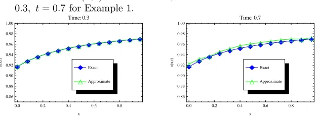
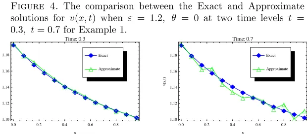
This numerical example is studied by using mesh sizeh= 0.05 and the time step ∆t = 0.01. The graphs of exact and numerical solutions at times t=0.3, 0.7 are demonstrated in Figures1-4for MQ and IMQ RBFs.
Tables3and 4respectively report the L2 andL∞ error norms between the exact and approximateuandvat t= 0.3 for some shape parameters.
Figure 1. The comparison between the Exact and Approximate solutions for u(x, t) when ε = 0.7, θ = 1 at two time levels t = 0.3, t= 0.7 for Example 1.
ì ì ì ì ì ì ì ì ì ì ì ì ì ó ó ó ó ó ó ó ó ó ó ó ó ó
0.0 0.2 0.4 0.6 0.8 0.86 0.88 0.90 0.92 0.94 0.96 0.98 1.00 x u H x ,t L Time: 0.3 ó Approximate
ì Exact ì ì ì ì ì ì ì ì ì ì ì ì ì ó ó ó ó ó ó ó ó ó ó ó ó ó
0.0 0.2 0.4 0.6 0.8 0.86 0.88 0.90 0.92 0.94 0.96 0.98 1.00 x u H x ,t L Time: 0.7 ó Approximate ì Exact
Figure 2. The comparison between the Exact and Approximate solutions for u(x, t) when ε = 1.2, θ = 0 at two time levels t = 0.3, t= 0.7 for Example 1.
ì ì ì ì ì ì ì ì ì ì ì ì ì ó ó ó ó ó ó ó ó ó ó ó ó ó
0.0 0.2 0.4 0.6 0.8 0.86 0.88 0.90 0.92 0.94 0.96 0.98 1.00 x u H x ,t L Time: 0.3 ó Approximate
ì Exact ì ì ì ì ì ì ì ì ì ì ì ì ì ó ó ó ó ó ó ó ó ó ó ó ó ó
0.0 0.2 0.4 0.6 0.8 0.86 0.88 0.90 0.92 0.94 0.96 0.98 1.00 x u H x ,t L Time: 0.7 ó Approximate ì Exact
Figure 3. The comparison between the Exact and Approximate solutions for v(x, t) when ε = 0.7, θ = 1 at two time levels t = 0.3, t= 0.7 for Example 1.
ì ì ì ì ì ì ì ì ì ì ì ì ì ó ó ó ó ó ó ó ó ó ó ó ó ó
0.0 0.2 0.4 0.6 0.8 1.12 1.14 1.16 1.18 x v H x ,t L Time: 0.3 ó Approximate ì Exact ì ì ì ì ì ì ì ì ì ì ì ì ì ó ó ó ó ó ó ó ó ó ó ó ó ó
0.0 0.2 0.4 0.6 0.8 1.12 1.14 1.16 1.18 x v H x ,t L Time: 0.7 ó Approximate ì Exact
In the problem (3.1)-(3.8) let
Du= 1, Dv= 4, ru=rv= 1, αuu=αvv =αuv=αvu= 1,
c1(t) =t, c2(t) =t2, c3(t) = 1, c4(t) = 1 +t2,
c5(t) =t, c6(t) = 1, c7(t) = 1, c8(t) =t2,
u(x,0) = sinx, φ1(t) =t2e−2t, ψ1(t) =e−2t(cos 1 +t2cos 1 + sin 1),
v(x,0) = cosx, φ2(t) =te−t, ψ2(t) =e−t(cos 1−t2sin 1),
F(x, t) =e−4tsinx(−2e2t+ttcosx+ sinx),
Figure 4. The comparison between the Exact and Approximate solutions for v(x, t) when ε = 1.2, θ = 0 at two time levels t = 0.3, t= 0.7 for Example 1.
ì ì
ì ì
ì ì
ì ì
ì ì
ì ì
ì
ó
ó ó
ó ó
ó ó
ó ó
ó ó ó
ó
0.0 0.2 0.4 0.6 0.8 1.10
1.12 1.14 1.16 1.18
x
v
H
x
,t
L
Time: 0.3
ó Approximate ì Exact
ì ì
ì ì
ì ì
ì ì
ì ì
ì ì
ì
ó
ó
ó ó
ó ó
ó ó ó
ó ó
ó ó
0.0 0.2 0.4 0.6 0.8 1.10
1.12 1.14 1.16 1.18
x
v
H
x
,t
L
Time: 0.7
ó Approximate ì Exact
Table 1. The L2 and L∞ error norms verses the shape parameter in Example 1 at t= 0.3 foru.
RBF shape parameter ε L2 error norm L∞ error norm MQ(θ= 1) 0.3 7.4976×10⁻³ 8.3831×10⁻³
0.5 3.0754×10⁻³ 4.9779×10⁻³ 0.7 3.0841×10⁻⁴ 4.8956×10⁻⁴ 0.9 7.9641×10⁻⁴ 9.4643×10⁻⁴ IMQ(θ= 0) 0.8 1.1081×10⁻² 2.5322×10⁻²
1 2.8643×10⁻³ 6.9851×10⁻³
1.2 1.8264×10⁻³ 3.5856×10⁻³ 1.4 5.6658×10⁻³ 8.1926×10⁻³
Table 2. The L2 and L∞ error norms verses the shape parameter in Example 1 at t= 0.3 forv.
RBF shape parameter ε L2 error norm L∞ error norm MQ(θ= 1) 0.3 5.1052×10⁻³ 8.2055×10⁻³
0.5 3.2728×10⁻³ 4.8362×10⁻³ 0.7 2.5789×10⁻⁴ 3.8771×10⁻⁴ 0.9 8.3597×10⁻⁴ 9.8853×10⁻⁴ IMQ(θ= 0) 0.8 4.4957×10⁻² 8.4498×10⁻²
1 5.9174×10⁻³ 9.9091×10⁻³
1.2 2.1228×10⁻³ 3.6093×10⁻³ 1.4 3.6001×10⁻³ 7.1818×10⁻³
With these assumptions the exact solutions may be derived as
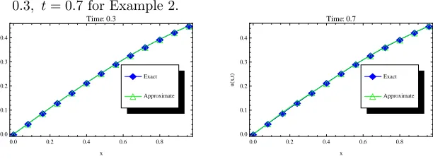
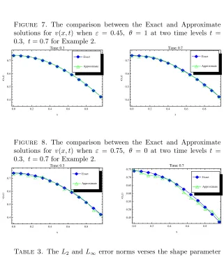
In this test problem we adopt our proposed numerical method using mesh sizeh= 0.05 and the time step ∆t= 0.01. Figures5-8show the exact and numerical solutions at timest= 0.3 andt= 0.7 for MQ and IMQ RBFs.
Figure 5. The comparison between the Exact and Approximate solutions for u(x, t) when ε = 0.45, θ = 1 at two time levels t = 0.3, t= 0.7 for Example 2.
ì ì ì ì ì ì ì ì ì ì ì ì ì ó ó ó ó ó ó ó ó ó ó ó ó ó
0.0 0.2 0.4 0.6 0.8 0.0 0.1 0.2 0.3 0.4 x u H x ,t L Time: 0.3 ó Approximate ì Exact ì ì ì ì ì ì ì ì ì ì ì ì ì ó ó ó ó ó ó ó ó ó ó ó ó ó
0.0 0.2 0.4 0.6 0.8 0.0 0.1 0.2 0.3 0.4 x u H x ,t L Time: 0.7 ó Approximate ì Exact
Figure 6. The comparison between the Exact and Approximate solutions for u(x, t) when ε = 0.75, θ = 0 at two time levels t = 0.3, t= 0.7 for Example 2.
ì ì ì ì ì ì ì ì ì ì ì ì ì ó ó ó ó ó ó ó ó ó ó ó ó ó
0.0 0.2 0.4 0.6 0.8 0.0 0.1 0.2 0.3 0.4 x u H x ,t L Time: 0.3 ó Approximate ì Exact ì ì ì ì ì ì ì ì ì ì ì ì ì ó ó ó ó ó ó ó ó ó ó ó ó ó
0.0 0.2 0.4 0.6 0.8 0.0 0.1 0.2 0.3 0.4 x u H x ,t L Time: 0.7 ó Approximate ì Exact
Tables3and 4respectively demonstrate the L2 andL∞ error norms between the exact and approximateuandv att= 0.3 for some shape parameters.
For this problem, rather than the previous problem, different shape parameters are obtained via our computation. Throughout the simulation, theL∞ andL2 error norms decrease with the smaller time step size. Similar to the test problem 1, the numerical results show that the effectiveness of the radial base functions MQ is better than IMQ for this problem.
5. Conclusion
Figure 7. The comparison between the Exact and Approximate solutions for v(x, t) when ε = 0.45, θ = 1 at two time levels t = 0.3, t= 0.7 for Example 2.
ì ì ì ì ì ì ì ì ì ì ì ì ì ó ó ó ó ó ó ó ó ó ó ó ó ó
0.0 0.2 0.4 0.6 0.8 0.4 0.5 0.6 0.7 x v H x ,t L Time: 0.3 ó Approximate
ì Exact ì ì ì ì ì ì ì ì ì ì ì ì ì ó ó ó ó ó ó ó ó ó ó ó ó ó
0.0 0.2 0.4 0.6 0.8 0.4 0.5 0.6 0.7 x v H x ,t L Time: 0.7 ó Approximate ì Exact
Figure 8. The comparison between the Exact and Approximate solutions for v(x, t) when ε = 0.75, θ = 0 at two time levels t = 0.3, t= 0.7 for Example 2.
ì ì ì ì ì ì ì ì ì ì ì ì ì ó ó ó ó ó ó ó ó ó ó ó ó ó
0.0 0.2 0.4 0.6 0.8 0.4 0.5 0.6 0.7 x v H x ,t L Time: 0.3 ó Approximate
ì Exact ì ì ìì ì ì ì ì ì ì ì ì ì ó ó ó ó ó ó ó ó ó ó ó ó ó
0.0 0.2 0.4 0.6 0.8 0.45 0.50 0.55 0.60 0.65 0.70 0.75 x v H x ,t L Time: 0.7 ó Approximate ì Exact
Table 3. The L2 and L∞ error norms verses the shape parameter in Example 1 at t= 0.3 foru.
RBF shape parameter ε L2 error norm L∞ error norm MQ(θ= 1) 0.35 6.0196×10⁻⁴ 8.4538×10⁻⁴
0.45 3.2592×10⁻⁴ 4.9309×10⁻⁴ 0.55 2.3935×10⁻³ 4.4225×10⁻³ 0.65 4.0121×10⁻² 7.9234×10⁻² IMQ(θ= 0) 0.65 7.8131×10⁻³ 9.067×10⁻³
0.75 3.5831×10⁻³ 4.7054×10⁻³ 0.85 2.1299×10⁻² 4.6571×10⁻² 0.95 4.4113×10⁻² 7.0605×10⁻²
Table 4. The L2 and L∞ error norms verses the shape parameter in Example 1 at t= 0.3 forv.
RBF shape parameter ε L2 error norm L∞ error norm MQ(θ= 1) 0.35 8.1516×10⁻⁴ 9.9703×10⁻⁴
0.45 4.4408×10⁻⁴ 5.1174×10⁻⁴ 0.55 3.3968×10⁻³ 5.7108×10⁻³ 0.65 5.2979×10⁻² 8.0093×10⁻² IMQ(θ= 0) 0.65 4.5425×10⁻³ 8.4608×10⁻³ 0.75 1.9729×10⁻³ 3.6828×10⁻³ 0.85 3.1964×10⁻² 4.7591×10⁻² 0.95 3.8838×10⁻² 7.9801×10⁻²
References
[1] D. G. Aronson, and H. F. Weinberger,Nonlinear diffusion in population genetics, combustion, and nerve pulse propagation, Lect. Not. Math.,446(1975), 549-563.
[2] R. S. Cantrell and C. Cosner,Spatial Ecology via Reaction-Diffusion Equations, Wiley, Chich-ester, England, 2003.
[3] C. Cosner,Reaction-Diffusion Equations and Ecological Modeling Tutorials in Mathematical Biosciences IV, Lecture Notes in Mathematics,1922(2008), 77–115.
[4] S. R. Dunbar, Travelling wave solutions of diffusive lotka-volterra equations, Math Bio., 17
(1983), 11-32.
[5] G. E. Fasshauer, J. G. Zhang,On choosing optimal shape parameters for RBF approximation, Numer. Algor.,45(2007), 345–368.
[6] B. Fornberg and C. Piret, On choosing a radial basis function and a shape parameter when solving a convective PDE on a sphere,J. Comput. Phys.,227(2008), 2758–2780.
[7] M. Garshasbi and M. Khakzad,The RBF collocation method of lines for the numerical solution of the CH-γequation, J. Adv. Res. Dyn. Cont. Sys.,4(2015), 65-83.
[8] E. E. Holmes, M. A. Lewis, J. E. Banks, and R. R. Veit,Partial differential equations in ecology: Spatial interactions and population dynamics Ecology, 75(1994), 17–29.
[9] Y. C. Hon and R. Schaback,On unsymmetric collocation by radial basis functions,Appl. Math. Comput.,119(2001), 177–186.
[10] S. Hubbert,Closed form representations for a class of compactly supported radial basis func-tions,Adv. Comput. Math.,36(2012), 115–136.
[11] J. Jones, P. J. Doran, and R. T. Holmes,Spatial scalling of avian population dynamics: Popu-lation abundance, groeth rate, and variability,Ecology,88(2007), 2505–2515.
[12] E. J. Kansa, Multiquadrics,A scattered data approximation scheme with applications to com-putational fluid-dynamics, I–Surface approximations and partial derivative estimates,Comput. Math. Appl.,19(1990), 127–145.
[13] A. La Rocca, A. Hernandez Rosales, and H. Power,Radial basis function Hermite collocation approach for the solution of time dependent convection–diffusion problems,Engin. Anal. Bound. Elem.,29(2005), 359–370.
[14] M. A. Lewis, B. T. Li, and H. E. Weinberger, Spreading speed and linear determinacy for two-species competition models, J. Math. Biol.,45(2002), 219–233.
[15] E. Lehto, V. Shankar, and G. B. Wright, A Radial Basis Function (RBF) Compact Finite Difference (FD) Scheme for Reaction-Diffusion Equations on Surfaces, SIAM J. Sci. Comput.,
39(2015), 2129–2151.
[16] J. Li, A. H. D. Cheng, and C. S. Chen,A comparisons of efficiency and error convergence of multiquadric collocation method and finite element method,Eng. Anal. Bound. Elem., 27
[17] F. Parzlivand and A. Shahrezaee,The use of inverse quadratic radial basis functions for the solution of an inverse heat problem,Bull. Iranian Math. Soc.,42(2016), 1127–1142.
[18] S. G. Rubin and R. A. Graves, Cubic spline approximation for problems in fluid mechanics, Nasa TR R-436, Washington, D. C., 1975.
[19] J. G. Skellam,Random disersal in theoretical populations, Biometrike, 38(1951), 196–218. [20] S. Toubaei, M. Garshasbi, and M. Jalalvand, A numerical treatment of a reaction-diffusion
model of spatial pattern in the embryo, Comput. Methods Differ. Equ.,4(2) (2016), 116–127. [21] J. Yoon, Spectral approximation orders of radial basis function interpolation on the Sobolev