www.geosci-model-dev.net/10/1889/2017/ doi:10.5194/gmd-10-1889-2017
© Author(s) 2017. CC Attribution 3.0 License.
Exploring precipitation pattern scaling methodologies and
robustness among CMIP5 models
Ben Kravitz1, Cary Lynch2, Corinne Hartin2, and Ben Bond-Lamberty2
1Atmospheric Sciences and Global Change Division, Pacific Northwest National Laboratory, Richland, WA, USA 2Joint Global Change Research Institute, Pacific Northwest National Laboratory, College Park, MD, USA
Correspondence to:Ben Kravitz ([email protected])
Received: 5 October 2016 – Discussion started: 23 November 2016
Revised: 29 March 2017 – Accepted: 29 March 2017 – Published: 12 May 2017
Abstract. Pattern scaling is a well-established method for approximating modeled spatial distributions of changes in temperature by assuming a time-invariant pattern that scales with changes in global mean temperature. We compare two methods of pattern scaling for annual mean precipitation (re-gression and epoch difference) and evaluate which method is “better” in particular circumstances by quantifying their robustness to interpolation/extrapolation in time, inter-model variations, and inter-scenario variations. Both the regression and epoch-difference methods (the two most commonly used methods of pattern scaling) have good absolute performance in reconstructing the climate model output, measured as an area-weighted root mean square error. We decompose the precipitation response in the RCP8.5 scenario into a CO2
portion and a non-CO2 portion. Extrapolating RCP8.5
pat-terns to reconstruct precipitation change in the RCP2.6 sce-nario results in large errors due to violations of pattern scal-ing assumptions when this CO2-/non-CO2-forcing
decompo-sition is applied. The methodologies discussed in this paper can help provide precipitation fields to be utilized in other models (including integrated assessment models or impacts assessment models) for a wide variety of scenarios of future climate change.
1 Introduction
Quantifying uncertainties in projections of climate change is one of the cornerstone investigative areas in climate science. There are numerous sources of uncertainty, including para-metric (which parameter values are the “right” ones), struc-tural (which key processes are missing or poorly
character-ized), and scenario (how climate-forcing agents will change in the future). One commonality among these sources is that uncertainties in each of them can be explored using climate models.
Atmosphere–ocean general circulation models (AOGCMs) are the gold standard of climate models used for projections of global change, as they incorporate many of the fundamentally climatically important processes, including atmosphere, land, ocean, and sea ice responses and feedbacks, as well as interactions between these different areas. However, their complexity means that these models are often computationally expensive, so any sensitivity studies or uncertainty quantification efforts using them are necessarily limited. No modern uncertainty quantification technique is capable of fully characterizing the space of AOGCM uncertainties and how they affect projections of climate change (Qian et al., 2016).
Pattern scaling has a fairly long history of research (e.g., Mitchell, 2003) and has been shown to be reasonably ac-curate for a variety of purposes. Lynch et al. (2017) pro-vided a review of pattern scaling of temperature, as well as an in-depth exploration of two commonly used pattern scal-ing methods (regression and epoch-difference methods, de-scribed later in Sect. 2.1). Both of these methods perform quite well in reproducing the actual model output for temper-ature. Conversely, comparatively little work has been done on pattern scaling for annual mean precipitation. Ruosteenoja et al. (2007) found that local precipitation changes are gener-ally linear with global mean temperature change, with errors of 15–30 % over 90 years of simulation. Holden and Edwards (2010) identified the importance of covariance between lo-cal temperature change and lolo-cal precipitation change, and Frieler et al. (2012) furthered this discovery, concluding that no single fit (e.g., regression coefficients) will be applicable to all grid points. Herger et al. (2015) used a novel method of piecing together results associated with the desired global mean temperature change and found excellent agreement with model output (errors rarely exceed 0.3 mm day−1). In a different style of emulation, Castruccio et al. (2014) trained a statistical model on pre-computed climate model simulations and found that it was capable of capturing nonlinearities in the response in ways that pattern scaling inherently cannot. Xu and Lin (2017) compared several different methods (akin to what we do in Sect. 4) to assess pattern scaling on temper-ature, precipitation, and potential evapotranspiration in the CESM Large Ensemble project (Kay et al., 2015). To the best of our knowledge, no previous study has compared different methods of pattern scaling of precipitation, particularly with a focus on robust model response.
Here we provide a systematic (although non-exhaustive) assessment of the robustness of pattern scaling of precipi-tation. Section 3 focuses on pattern scaling the response to temperature changes solely due to carbon dioxide increases, looking at interpolation in time, extrapolation in time, and inter-model robustness. Section 4 explores inter-scenario ro-bustness; i.e., whether the patterns obtained for CO2are
use-ful for pattern scaling other scenarios.
Through these investigations, we hope to better reveal in what circumstances methods of pattern scaling of precipita-tion perform well. We will also provide some (limited) guid-ance as to which situations pattern scaling is likely to provide a computationally efficient, reasonably accurate result vs. which situations require actual simulation using AOGCMs.
2 Pattern scaling methods
2.1 Two methods of pattern scaling for precipitation Pattern scaling involves approximating a time series of the pattern of change in a field of interest1B(x, t )by1B(ˆ x, t ): 1B(x, t )≈1B(ˆ x, t )=P (x)1T (t ),¯ (1)
where P (x) describes a time-invariant spatial pattern (the spatial dimension is denoted byx), and1T (t )¯ describes a time-varying (the time dimension is denoted byt) series of the change in global mean temperature, starting from a refer-ence periodt=0 (often the preindustrial era). This notation will be used repeatedly throughout the paper. There are two commonly used methodologies for ascertaining P (x): re-gression and epoch differencing (Barnes and Barnes, 2015). In the regression method, P (x) is obtained by regressing 1B(x, t )=B(x, t )−B(x,0)against1T (t )¯ at each point in x. In the epoch method,
P (x)=B (x,[k, n+k])−B (x,[0, n]) ¯
T ([k, n+k])− ¯T ([0, n]) , (2) where the intervals [0, n]and [k, n+k] indicate averaging overn-year time periods at the beginning and end of the sim-ulation, respectively. All values calculated are over a multi-model mean; Ruosteenoja et al. (2007) showed that pattern scaling for precipitation over a model mean outperforms re-sults obtained from using single models. Frieler et al. (2012) argued that no single set of regression coefficients will be ap-plicable to all grid points. We circumvent this issue by (for example) regressing1T¯ against1Bat each grid point. 2.2 Methodology
In the following sections, we quantify differences between the reconstructionBˆ and the actual model outputB via the root mean square (rms) over the area-weighted difference
ˆ
B−B, calculated as
rms= r P x h ˆ
B(x)−B(x)
·A(x)
i2
q P
x[A(x)]2
, (3)
whereA(x)is the area of grid boxx, and sums are calculated over allx.
All of the analysis conducted here uses simulations from AOGCMs contributed to CMIP5. The models used in the bulk of the analysis in this study (Table 1, group 1) are iden-tical to those used by Lynch et al. (2017) with two exceptions (due to model output availability):
1. The present study used NorESM1-ME instead of NorESM1-M. NorESM1-ME includes prognostic bio-geochemical cycling and has the capability of being emissions driven, but when using concentration-driven scenarios (as is the case here), the two versions of the model will produce nearly identical results (Bentsen et al., 2013).
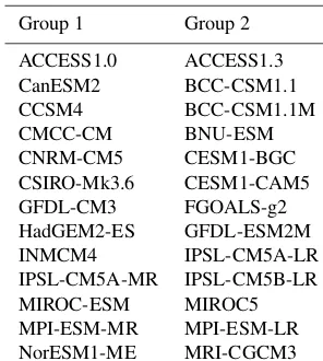
Table 1.Models used in the present analysis. Most of the analysis was conducted using the models in group 1. Additional investiga-tions described in Sect. 3.3 were conducted using the models in both group 1 and group 2 to determine inter-model robustness of the dif-ferent pattern scaling methods discussed in this study. All model names listed are the standard names used in contributions to the Coupled Model Intercomparison Project Phase 5 (CMIP5; Taylor et al., 2012). Knutti et al. (2013) provide an excellent description of these models and their provenance.
Group 1 Group 2
ACCESS1.0 ACCESS1.3 CanESM2 BCC-CSM1.1 CCSM4 BCC-CSM1.1M CMCC-CM BNU-ESM CNRM-CM5 CESM1-BGC CSIRO-Mk3.6 CESM1-CAM5 GFDL-CM3 FGOALS-g2 HadGEM2-ES GFDL-ESM2M INMCM4 IPSL-CM5A-LR IPSL-CM5A-MR IPSL-CM5B-LR MIROC-ESM MIROC5 MPI-ESM-MR MPI-ESM-LR NorESM1-ME MRI-CGCM3
(Davini et al., 2014; Sanna et al., 2013). Cagnazzo et al. (2013) described some of the differences between these two models. In general, the models agree on qualita-tive climate features, although as might be expected, CMCC-CMS better matches observations in situations where a fully resolved stratosphere is important for cap-turing the effects, including dynamical feedbacks of stratospheric circulation and ozone chemistry on surface climate. Although these effects are non-negligible, they are generally of lower order than the changes that occur over the course of the scenarios analyzed in this study (to be discussed presently); therefore, we anticipate that differences between these two models will not substan-tially affect results for the model mean.
These models were chosen to be representative of the CMIP5 ensemble while retaining model independence; Lynch et al. (2017) described more of the details as to why those models were chosen.
Throughout this study, we evaluate three scenarios. The 1pctCO2 scenario involves a 1 % per year increase in the CO2concentration, beginning at its preindustrial value. This
simulation is run for 140 years to an approximate quadru-pling of the CO2 concentration. The RCP8.5 and RCP2.6
scenarios (Representative Concentration Pathways, or RCPs; Moss et al., 2010; Meinshausen et al., 2011) describe the re-sults of two socioeconomic narratives that produce particu-lar concentration profiles of greenhouse gases, aerosols, and other climatically relevant forcing agents over the 21st cen-tury. The RCP8.5 scenario reflects a “no policy” narrative,
Table 2.Radiative-forcing values (W m−2) for RCP8.5 and RCP2.6 in 2000, 2050, and 2100. CO2forcing and total forcing were
calcu-lated using the simple climate model Hector (Hartin et al., 2015). Non-CO2forcing is calculated as the difference between total and
CO2forcing. Percentages in parentheses indicate the percentage of the total forcing.
2000 2050 2100
CO2forcing (RCP8.5) 1.226 3.289 6.167 Total forcing (RCP8.5) 1.991 5.049 8.686 Non-CO2forcing (RCP8.5) 0.765 (38 %) 1.760 (35 %) 2.519 (29 %)
CO2forcing (RCP2.6) 1.267 2.174 1.765 Total forcing (RCP2.6) 2.066 3.195 2.601 Non-CO2forcing (RCP2.6) 0.799 (39 %) 1.021 (32 %) 0.836 (32 %)
in which total anthropogenic forcing reaches approximately 8.5 W m−2 in the year 2100. Conversely, the RCP2.6 sce-nario involves aggressive decarbonization, causing radiative forcing to peak at approximately 3 W m−2around 2050 and decline to approximately 2.6 W m−2 at the end of the 21st century. Table 2 provides additional forcing details for the two RCP scenarios, as calculated by Hector (Hartin et al., 2015), a climate, carbon-cycle model that is used as the cli-mate component of the Global Change Assessment Model (GCAM), a state-of-the-art Integrated Assessment Model. Both RCPs are appended to simulations of the historical pe-riod, for total simulation lengths of 251 years (1850–2100).
Throughout the remainder of the paper, subscripts onP, ¯
T,Bˆ, andBare used to denote the scenario (e.g., RCP8.5), the model group (e.g., group 2), or the years over which the patterns are computed (e.g., 1–50). If there is no sub-script specified, then the associated value corresponds to the group 1 (see Table 1) multi-model mean of the 1pctCO2 sim-ulation, averaged over years 116–140 of the simulation (the last 25 years of the 1pctCO2 simulation, approximately at quadruple the preindustrial CO2concentration).
Statistical significance was calculated using Welch’sttest, which is analogous to a Student’st test, but where the vari-ancess1ands2of the two samplesx1 andx2, respectively,
do not need to be equal. We use this statistic here because the ensemble for each method is small, and the ensemble pat-tern distribution is assumed to be normal. The test statistic is defined by
t= x¯1− ¯x2 q
s12/n1+s22/n2
, (4)
wheren1andn2 are the number of models in each sample,
ap-Table 3. The rms error values calculated over the entire globe (Eq. 3) for each of the figures. All units are in mm day−1for differ-ences (Figs. 3, 6, 7, 10, 11, and 12) or mm day−1K−1for patterns (Fig. 5).
Regression Epoch difference
Figure 3 0.04 0.03
Figure 5 0.02 0.02
Figure 6 0.10 0.10
Figure 7 0.09 0.09
Figure 10 0.10 0.07
Figure 11 0.10 0.09
Figure 12 0.21 0.20
proximated by the Welch–Satterthwaite equation:
df = s 2
1/n1+s22/n2 2
s2 1/n1
2 n1−1 +
s2 2/n2
2 n2−1
. (5)
In all figures, stippling is used to obscure values that are not statistically significant; i.e., thetstatistic failed to exceed the 95 % confidence threshold.
3 Comparisons between pattern scaling methods for CO2-only forcing
3.1 Pattern scaling for CO2concentration changes Figure 1 shows the baseline (preindustrial) annual mean pre-cipitation pattern B(x,0)and the scaling patternsP (x)for both of the pattern scaling methods generated from the group 1 (see Table 1) model average for the 1pctCO2 simulation. The regression and epoch-difference methods have very sim-ilar scaling patterns, no differences greater in magnitude than 0.05 mm day−1K−1, and no differences are statistically sig-nificant (not shown). Both patterns show similar broad fea-tures: an increase in tropical precipitation with global warm-ing, particularly over the oceans; increases at high latitudes, again over the oceans; and decreases in the South Pacific, North Atlantic, and southern Indian oceans, as well as Cen-tral America and the Mediterranean basin.
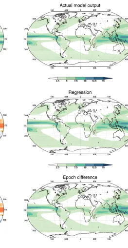
Figure 2 shows a comparison between the actual model output (group 1 averaged over the mean of years 116–140 of the 1pctCO2 simulation) and the two methods of recon-struction. Both methods show qualitatively similar features. In general, they reproduce the actual model output well, with possible exceptions in the tropics. Tebaldi and Arblaster (2014) noted that pattern scaling methodologies have diffi-culty in representing convection processes; therefore, depar-tures in these areas might be expected.
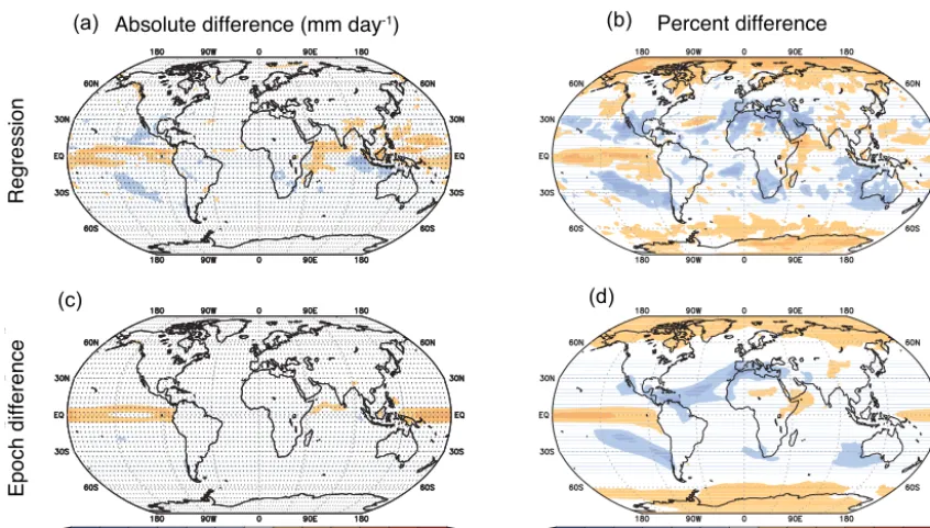
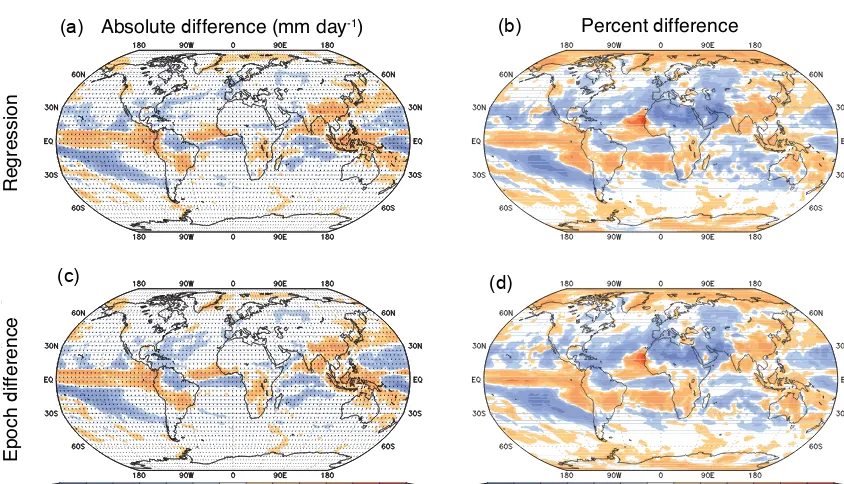
Figure 3 shows a more quantitative comparison be-tween the different reconstruction methods and the actual model output. Overall error (rms; Eq. 3) in the regres-sion and epoch-difference methods are very small (0.04 and
0.03 mm day−1, respectively; see Table 3), and no region in the reconstruction is statistically different from the actual model output.
3.2 Interpolation/extrapolation
In this section, we examine robustness of the methods to interpolation or extrapolation in time. If the scaling pattern P (x)truly were time invariant, then the results presented in this section would be identical to those previously discussed. Supplement Fig. S1 shows the patternsP (x)obtained by conditioning the reconstructions only on years 1–50 of the 1pctCO2 simulation. In the epoch-difference method, the second epoch is calculated over years 26–50 instead of years 116–140. In the regression method, the regression coeffi-cients are calculated only using the first 50 years of simu-lation. The patterns calculated by using the regression and epoch-difference methods only show small changes between the two periods, virtually none of which is statistically sig-nificant.
Despite similarities, using patterns conditioned on the ear-lier period to reconstruct the precipitation in the later pe-riod (years 116–140) results in considerably poorer perfor-mance for both methods (Supplement Fig. S2) than the re-sults shown in Fig. 3. The rms error increases by an order of magnitude (not shown), although few areas show statis-tically significant differences from the actual model output over this time period. This is likely due to the noise intro-duced by buildingP (x)on the early years of the simulation when the climate change signal is weak.
Figure S3 in the Supplement shows results for interpola-tion in time, where the patterns are condiinterpola-tioned on the full 1pctCO2 simulation (years 116–140), but the reconstruction predicts the average temperature in years 58–82 (halfway through the 1pctCO2 simulation). More specifically, Bˆ= P116−140(x)1T (¯ 58−82). In general, the patterns for
inter-polation show similar qualitative features to those of recon-structing the later time period of years 116–140 (Fig. 3). However, error increases by a factor of 2 for both methods, which potentially indicates the presence of nonlinearity. As before, no difference is statistically significant.
3.3 Inter-model robustness
Baseline
Regression
Epoch difference
Figure 1.The components needed for pattern scaling of the pre-cipitation response to CO2forcing, averaged over the 13 models in
group 1 (Table 1). Top shows the baseline precipitation pattern for the multi-model average:B(x,0)in Eq. (1) (mm day−1; averaged over years 1–25 of the 1pctCO2 simulation). The other panels show the time-invariant patternP (x)in Eq. (1) (mm day−1K−1) for the regression method (middle) and the epoch-difference method (bot-tom).
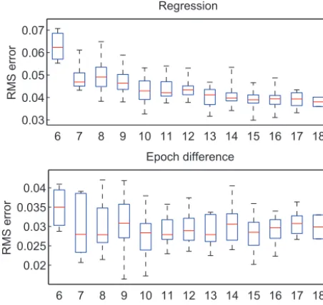
Figure 4 shows the rms error in the reconstruction (1pctCO2 simulation, averaged over years 116–140) as a function of the number of models used in the comparison.
Actual model output
Regression
Epoch difference
Figure 2.Comparison between the actual group 1 multi-model av-erage precipitation output (top) and the reconstructions produced by pattern scaling (Bˆ in Eq. 1). All values are in mm day−1 and
represent averages over years 116–140 of the 1pctCO2 simulation. Middle panel shows the regression method, and bottom panel shows the epoch-difference method.
Regression
Epoch
d
ifference
Absolute difference (mm day-1) Percent difference
(a) (b)
(c) (d)
Figure 3. Differences between the reconstructions produced by pattern scaling (B) and the actual model output for precipitation (B).ˆ
(a)shows absolute values ofBˆ−B (mm day−1), and (b)shows percent change. Top row shows results for the regression method, and bottom row shows the epoch-difference method. All values are calculated for a group 1 multi-model average for the 1pctCO2 simulation over the years 116–140. Stippling indicates a lack of statistical significance in the pattern of differences (Sect. 2.2).
this figure parallel those discussed in previous sections: both methods have similar magnitudes of error (except for small numbers of models). The rms error values (Table 3) for group 1 (13 models) are consistent with the rms error ranges de-picted in Fig. 4, indicating that group 1 is not an outlier.
The regression method shows a dependence of rms error on the number of models, whereas with the exception of low model numbers (<10), there is much lower dependence for the epoch method. However, except for low model numbers, none of the boxes/whiskers is substantially different from any of the others, leading us to conclude that each of the methods is largely robust to changes in the number of models used to carry out pattern scaling. Section 2 in the Supplement and the associated figures provide additional comparisons between the patterns generated for groups 1 and 2.
3.4 Discussion of pattern scaling the precipitation response to CO2
Both the regression and epoch-difference methods show great promise in their usefulness as precipitation pattern scal-ing methods. Both are able to reconstruct the changes in pre-cipitation due to CO2increases with errors of less than 5 %
in every region of the globe (Fig. 3). However, when exam-ining interpolation in time, error increases for both meth-ods, indicating issues with robustness to timescale (Supple-ment Sect. S1). Also, the pattern shows increased error in
many places when different models are used (Supplement Sect. S2), indicating issues with inter-model robustness.
Like the temperature pattern scaling results of Lynch et al. (2017), we find that the regression and epoch-difference methods have similar performance. In the present work, we find that the epoch-difference method slightly outperforms the regression method, but the differences are relatively mi-nor. Given the slight advantages in computational expense and reduced data input requirements, we profess a slight preference for using the epoch-difference method to gener-ate scaling patterns for the precipitation response to CO2
-induced global warming.
4 Pattern scaling for additional forcings
In this section, we compare the patterns and reconstruc-tions between scenarios, primarily related to the RCP8.5 and 1pctCO2 simulations. We do this first as a test of robust-ness: do the pattern scaling methods perform “better” for CO2-only simulations vs. RCP8.5? If the fidelity of the
re-construction to the actual model output is similar for the two scenarios, then subtracting the reconstructions conditioned on RCP8.5 and 1pctCO2 could reveal a scaling pattern for non-CO2forcing. We note that this is one of the few ways
of ascertaining the non-CO2 response pattern without
run-ning separate simulations both with and without CO2
re-0.03 0.04 0.05 0.06 0.07
6 7 8 9 10 11 12 13 14 15 16 17 18
RMS error
Regression
0.02 0.025 0.03 0.035 0.04
6 7 8 9 10 11 12 13 14 15 16 17 18 Number of models
RMS error
Epoch difference
Figure 4.Root mean square (rms) error (Eq. 3, calculated on the difference expressed in mm day−1between the reconstruction and actual model outputBˆ−B) as a function of the number of models used to conduct the scaled precipitation reconstruction. From the full set of 26 models (Table 1), anywhere between 6 and 18 mod-els (xaxis) were chosen randomly 20 different times. Each box in the plots represents those 20 sets of models. Red lines indicate me-dian values, blue boxes indicate the 25th and 75th percentiles, and whiskers indicate the full range of model response among the 20 sets of models. All values are calculated over an average of years 116–140.
sults from directly subtracting a 1pctCO2 simulation from an RCP8.5 simulation. (The approach discussed here is anal-ogous to the methodology of Herger et al., 2015, but where they attempted to ascertain similarities between patterns for a given change in global mean temperature, we are interested in the differences.)
We note several caveats with this approach. One is that, based on the results of Herger et al. (2015), the reconstruc-tions of RCP8.5 and 1pctCO2 are likely to have some simi-larities for a given temperature change because the dominant forcing in RCP8.5 is CO2 (see Table 2). Therefore,
ascer-taining the non-CO2 signal could be limited by low
signal-to-noise ratios. A second caveat, one more germane to pat-tern scaling, is to ascertain whether the non-CO2pattern
ob-tained from RCP8.5 can be used to reconstruct the non-CO2
precipitation change for a different scenario. There is no a priori reason to expect that this will work, as different sce-narios have different combinations of forcings. In Sect. 4.3, we investigate this problem using an extreme case, where we ascertain the scaling patterns from an RCP8.5 simulation and use them to attempt to reconstruct the RCP2.6 simulation.
We acknowledge that the non-CO2component is a
com-bination of both non-CO2 greenhouse gases and aerosols,
which have opposite effects on global mean temperature. These two categories of forcing have different local re-sponses as well. An alternative approach would be to split the RCP8.5 response into a CO2 component, a non-CO2
greenhouse gas component, and a non-greenhouse gas com-ponent. Supplement Sect. S3 discusses the necessary calcu-lations for both of these approaches. The CO2/non-CO2
ap-proach proved to be quite amenable to pattern scaling. On the contrary, the CO2/other greenhouse gas/non-greenhouse gas
approach is not, due to distinct nonlinear relationships be-tween the precipitation response and the derived temperature responses for these particular forcing categories. Therefore, we have chosen to proceed with a CO2/non-CO2division for
the purpose of pattern scaling.
4.1 Inter-scenario differences
Figure 5 shows the RCP8.5 scaling pattern PRCP8.5(x)
and the difference from the CO2-only pattern. Patterns are
nearly identical to those in Fig. 1. Both the regression and epoch-difference methods show no differences exceeding 0.1 mm day−1K−1in magnitude and no statistically signifi-cant differences of any magnitude. This figure reinforces the findings of Herger et al. (2015) that patterns generated from commonly used scaling methods (regression and epoch dif-ference) do not differ appreciably between scenarios; there-fore, pattern scaling can be accomplished by using periods in different scenarios with the same global mean temperature change.
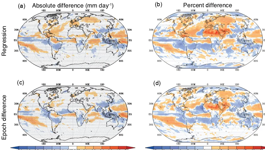
Figures 6 and 7 show this in practice, where the recon-struction of the historical/RCP8.5 simulationBˆ is built on the RCP8.5 pattern, multiplied by1T¯ averaged over years 227–251 (2076–2100) and 116–140 (1965–1990), respec-tively. The reconstructed precipitation response in Figure 6 is generally too strong in the tropics and too weak in the midlatitudes (which is the same pattern in Fig. 3), but Fig. 7 shows the opposite pattern. None of these differences is sta-tistically significant, and the rms error is approximately the same in both figures (0.09–0.10 mm day−1K−1; 2–3 times greater than the error in Fig. 3), but they suggest that there is a distinct non-CO2pattern that, while small, is still important
in explaining precipitation differences in periods with large temperature change.
4.2 Non-CO2-forcing pattern
Here we calculate a non-CO2pattern for use in pattern
scal-ing. We begin by assuming that the effects of CO2 forcing
and non-CO2 forcing are separable; i.e., there are no
Regression
Epoch
d
ifference
PRCP8.5 PRCP8.5 – P1pctCO2
(a) (b)
(c) (d)
Figure 5.Absolute values (left) of and differences (right) in the precipitation scaling patternP (x)(Eq. 1) when different scenarios are used to construct the pattern (RCP8.5 vs. 1pctCO2). Panels(a, c)show values ofPRCP8.5, and(b, d)show values ofPRCP8.5−P1pctCO2
(mm day−1K−1). Panels(a, b)show results for the regression method, and bottom row shows the epoch-difference method. All values are calculated for a group 1 multi-model average for the 1pctCO2 simulation. Stippling indicates a lack of statistical significance in the pattern of differences (Sect. 2.2).
Regression
Epoch
d
ifference
Absolute difference (mm day-1) Percent difference
(a) (b)
(c) (d)
Figure 6. As in Fig. 3 but where the reconstruction Bˆ is built on the pattern P for the RCP8.5 simulation (group 1 average over years 227–251), and global mean temperature 1T¯ is averaged over years 227–251 (2076–2100) of the RCP8.5 simulation; i.e., Bˆ = PRCP8.5(x)1T¯RCP8.5(227–251). Results shown are for the difference between the reconstruction and the actual model output of the RCP8.5
Regression
Epoch
d
ifference
Absolute difference (mm day-1) Percent difference
(a) (b)
(c) (d)
Figure 7.As in Fig. 3 but where the reconstructionBˆ is built on the patternP for the RCP8.5 simulation (group 1 average over years 227–251), and global mean temperature1T¯ is averaged over years 116–140 (1965–1990) of the historical/RCP8.5 simulation; i.e.,Bˆ = PRCP8.5(x)1T¯RCP8.5(116–140). Results shown are for the difference between the reconstruction and the actual model output of the historical
simulationBˆ−B
RCP8.5(x,116–140).
200 400 1000 1200
−1 0 1 2 3 4 5 6
600 800
CO
2concentration (ppm)
Temperature
c
hange (K)
1pctCO2 RCP8.5 RCP8.5 (CO
2 part) RCP8.5 (non−CO
2 part)
Figure 8.Decomposition of global mean temperature change (as a function of the CO2concentration) into its components, as
de-scribed in Sect. 4.2.
Eq. (1), separability means that
1BˆRCP8.5=1T¯CO2PCO2+1T¯non−CO2Pnon−CO2. (6) We setPCO2 equal toP1pctCO2 (from Sect. 3), because if pattern scaling holds, the time-invariant pattern of CO2
forc-ing should be identical, regardless of the scenario from which it is derived.Pnon−CO2is defined to be 4PRCP8.5−3PCO2(see Sect. S3 in the Supplement for the derivation of this
expres-sion). Embedded in this expression are inherent assumptions about the validity of a linear pattern scaling approach. If the approach fails, it is because either this pattern does not rep-resent actual non-CO2forcing or because the pattern is too
difficult to accurately estimate, perhaps due to internal vari-ability. We also note that because this end result is the differ-ence of two large quantities, it may be sensitive to noise that occurs in eitherPRCP8.5orPCO2.
To calculate1T¯CO2, we assume that global mean tempera-ture scales linearly with radiative forcing (e.g., Gregory et al., 2004), and radiative forcing is known to scale logarithmically with the CO2concentration (Myhre et al., 1998). Performing
linear regression of log2([CO2])against global mean
tem-perature change in the 1pctCO2 simulation yields a slope of α=2.40, an intercept ofβ= −19.89, and an R2 value of 0.99. (Brackets[·]indicate the CO2concentration in ppmv.)
Then1T¯CO2=αlog2([CO2])+β.1T¯non−CO2 is calculated as the residual1T¯RCP8.5−1T¯CO2. We note that this formu-lation does not explicitly account for lags in the climate re-sponse to radiative forcing such as ocean thermal inertia.
Figure 8 shows all of the aforementionedT¯ values, plotted as a function of the CO2concentration. Both CO2and
non-CO2monotonically increase with time in the RCP8.5
simu-lation. This is consistent with the design of the RCP8.5 sce-nario, in which non-CO2radiative forcing increases over the
forc-Regression Epoch difference
CO
2
p
art
Non-CO
2
p
art
Non-CO
2
p
art
minus CO
2
part
(a) (b)
(c) (d)
(e) (f)
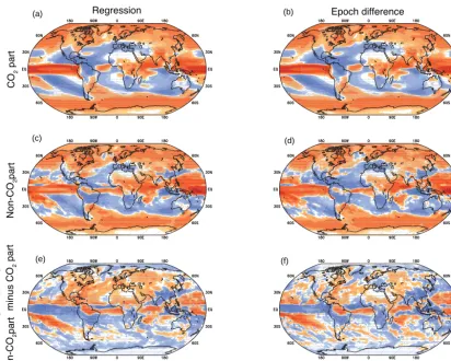
Figure 9.The CO2(a, b)and non-CO2(c, d)responses over years 227–251 (2076–2100) of the RCP8.5 simulation, as well as the
dif-ference between the two(e, f). CO2response is calculated as1Bˆ=P
1pctCO21T¯RCP8.5(227–251), and non-CO2response is calculated as
1Bˆ=Pnon−CO21 ¯
TRCP8.5(227–251) (see Eq. 1 and the discussion surrounding Eq. 6 for further details). Left column shows results for the
regression method and right column shows the epoch-difference method.
ing corresponds to a non-CO2-induced temperature change
(green line in Fig. 8) from 0.31 to 1.36 K.
Figure 9 provides descriptions of the actual precipita-tion effects of both CO2 and non-CO2 forcing. Although
the two portions of the reconstruction generally show sim-ilar features, the regional effects have quite different magni-tudes in many regions. In particular, the non-CO2 response
is weaker over the tropical Pacific than the CO2 response
and is stronger over much of the Northern Hemisphere. One distinct difference between the two patterns is that precipi-tation is reduced over East Asia and India in the non-CO2
response but increases in the CO2response. This is likely a
result of global dimming from heavy aerosol emissions. An-other source of differences, potentially attributable to dust, is the Saharan outflow over the Atlantic Ocean and extending into the Amazon. This gives us confidence that although the non-CO2 response is likely dominated by non-CO2
green-house gases (most prominently methane), it appears to have captured an aerosol signature. It would be a useful future area of investigation to conduct pattern scaling studies on
single-forcing simulations (e.g., Marvel et al., 2016) to reveal more robust signals and determine which forcings are amenable to pattern scaling, with a particular eye on inter-model vari-ations in the responses to identical forcings. The results in Fig. 9 also reinforce the conclusions of Frieler et al. (2012), who argue that the scaling patterns from one scenario are not in general translatable to scaling patterns for another scenario if the two scenarios are driven by different forcing. Even though Fig. 5 shows that the patternsPRCP8.5andP1pctCO2
are nearly identical, even small differences can affect recon-structions of precipitation change for large values of1T¯.
This decomposition of the scaling patterns into CO2 and
non-CO2components performs rather well for
Regression
Epoch D
d
ifference
Absolute difference (mm day-1) Percent difference
(a) (b)
(c) (d)
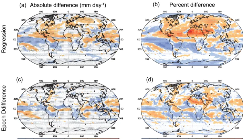
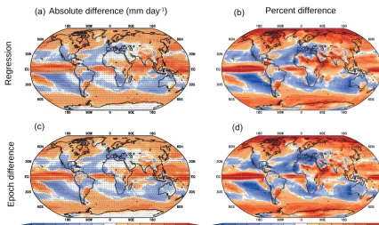
Figure 10.As in Fig. 3 but where1Bˆ=Pnon−CO21 ¯
TRCP8.5,nonCO2(227–251)+P1pctCO21 ¯
TRCP8.5,CO2(227–251), and results are shown for1Bˆ−1BRCP8.5(227–251). (See Eq. 1 and the discussion surrounding Eq. 6 for details.)
Regression
Epoch
d
ifference
Absolute difference (mm day-1) Percent difference
(a) (b)
(c) (d)
Figure 11.As in Fig. 3 but where1Bˆ=Pnon−CO21 ¯
TRCP8.5,nonCO2(116–140)+P1pctCO21 ¯
TRCP8.5,CO2(116–140), and results are shown for1Bˆ−1BRCP8.5(116–140). (See Eq. 1 and the discussion surrounding Eq. 6 for details.)
the period 1965–1990 (Fig. 11), both methods perform nearly identically with slight (<0.2 mm day−1) biases in the
trop-ics, East Asia, Europe, and the South Pacific. The errors in Fig. 10 are generally of the opposite sign of those in Fig. 6, and some of the features in Fig. 11 are of the opposite sign of
those in Fig. 7. This indicates that some features of non-CO2
response offset features of the CO2response. Particular areas
Regression
Epoch
d
ifference
Absolute difference (mm day-1) Percent difference
(a) (b)
(c) (d)
Figure 12.As in Fig. 3 but where1Bˆ=P
non−CO21T¯RCP2.6,nonCO2(227–251)+P1pctCO21T¯RCP2.6,CO2(227–251), and results are shown for1Bˆ−1BRCP2.6(227–251). (See Eq. 1 and the discussion surrounding Eq. 6 for details.)
4.3 Scaling to predict other scenarios
The final stage of inter-model exploration is to see how well the CO2and non-CO2patterns generated from one scenario
can be used on another scenario. Here we choose the ex-treme case of predicting the pattern of precipitation change in RCP2.6, based on the patterns calculated from RCP8.5. In this scenario, the CO2concentration peaks and then drops
slightly (Table 2). The non-CO2forcing comprises 29 % of
the total forcing in RCP8.5 in 2100 and 32 % of the total forcing in RCP2.6 in 2100, according to simulations using Hector (Hartin et al., 2015).
Figure 12 shows the effectiveness of this reconstruction process. Both the epoch-difference and regression methods show strong differences that are consistent with the patterns displayed in Fig. 9. Section S4 in the Supplement provides some additional derivations that explore the sources of these biases. There are two main conclusions from this section. First, using the non-CO2 pattern build on RCP8.5 was not
effective for explaining non-CO2behavior in RCP2.6,
indi-cating that there are limits to the applicability of a “univer-sal” non-CO2 forcing. A future area of investigation could
explore these limits: for example, would the non-CO2
pat-tern built on RCP8.5 work on RCP6.0 or RCP4.5 instead of the extreme RCP2.6 case? The second conclusions is that the ability to perform this CO2/non-CO2decomposition is itself
limited. Supplement Sect. S4 goes through detailed calcula-tions showing that if one assumes that such a decomposition is possible, contradictions and inconsistencies arise.
Deter-mining why this decomposition failed for RCP2.6 would re-quire a more thorough investigation, possibly including sin-gle forcing simulations, which is beyond the scope of this study. Such research could lead to an understanding of which scenarios would be more amenable to separable forcing treat-ments than others.
4.4 Discussion of pattern scaling for non-CO2forcings In general, the pattern scaling results depicted in Sect. 4 are consistent with previous studies. Herger et al. (2015) found that the patterns between scenarios are rather similar, which Fig. 5 confirms. However, the results for pattern scaling may be scenario dependent (Fig. 9) if global mean temperature change(1T )¯ is sufficiently large, which confirms the con-clusions of Frieler et al. (2012).
In particular, we found limited ability in reconstructing the RCP2.6 model behavior from the RCP8.5 run, indicating limits in building scalings using one scenario and applying them to a different scenario. We deliberately chose an ex-treme case to understand whether such universal applications exist. The ability to do this might be improved for “closer” scenarios, such as RCP8.5 and RCP6.0 or RCP4.5.
5 Conclusions
variations, and inter-scenario differences. Both the regres-sion and epoch-difference methods perform well and approx-imately similarly.
Most of the errors that arise for either method are either in areas dominated by convection (predominantly over the trop-ical oceans) or at high latitudes. Both of these areas are large sources of nonlinear responses to global mean temperature change; therefore, pattern scaling might not be expected to perform well in these areas. The approach of Tebaldi and Ar-blaster (2014) of using zonal mean temperature as a scaling parameter may prove useful in accounting for errors at high latitudes.
In terms of the usefulness of pattern scaling of precipita-tion, because the regression and epoch-difference methods perform well over most land regions, they are likely quite suitable for a variety of applications, including societal mod-els (like integrated assessment modmod-els or impacts modmod-els) that mostly deal with land areas. If one’s application requires good performance over tropical oceans, then pattern scaling may no longer be appropriate, and instead output from the full AOGCM may be required. However, given the difficul-ties that many climate models have with proper representa-tions of convective processes and the resulting precipitation biases those difficulties cause (e.g., Song and Zhang, 2009), there may be doubts as to how well AOGCMs represent pre-cipitation in these areas in the first place.
The results presented in Sect. 4 indicated that while some scenarios are amenable to broad separations of pattern scal-ing forcscal-ings, some others are not. Much more systematic work needs to be done in this area to determine the useful-ness of pattern scaling for different forcings. Single forcing experiments would be particularly useful, as they can allow for a determination as to which forcings work best for pattern scaling, as well as whether there are any nonlinear effects that result from applying multiple simultaneous forcings. An-other potential approach would be to use the “hybrid-pattern” method described by Xu and Lin (2017), in which a simple energy balance model is used to build separate forcings, cir-cumventing the need for expensive single-forcing AOGCM simulations.
The results presented here have applications that extend beyond providing libraries of scaling patterns for integrated assessment models (Lynch et al., 2017). Another more spec-ulative application involves efficacy of climate forcings. Kravitz et al. (2015) developed a method of comparing forc-ing agents via analyses of their rapid adjustments (fast re-sponses), i.e., their responses in the absence of global mean temperature change. If our method of decomposing the re-sponse into CO2 and non-CO2 components could be
ex-tended to single forcings, then one could isolate the feedback responses (slow responses), which are the portions of the responses that depend on global mean temperature change. Thus, there is potential to provide a more quantitative inter-comparison of the different effects of climate forcing agents.
Code and data availability. All computations were performed us-ing MATLAB 2012b, developed by MathWorks. The libraries of patterns are available on GitHub at http://github.com/JGCRI/ CMIP5_patterns. All code used to generate figures in this paper is available upon request.
The Supplement related to this article is available online at doi:10.5194/gmd-10-1889-2017-supplement.
Author contributions. All authors collectively designed the study. B. Kravitz was the lead on conducting analysis and writing the pa-per, with input from the other authors at all stages.
Competing interests. The authors declare that they have no conflict of interest.
Acknowledgements. The authors thank two anonymous reviewers for their help in improving the manuscript. This research is based on work supported by the US Department of Energy, Office of Science, Integrated Assessment Research Program. We acknowl-edge the World Climate Research Programme’s Working Group on Coupled Modeling, which is responsible for CMIP, and we thank the climate modeling groups for producing and making available their model output. For CMIP the U.S. Department of Energy’s Program for Climate Model Diagnosis and Intercomparison provides coordinating support and led development of software infrastructure in partnership with the Global Organization for Earth System Science Portals. The Pacific Northwest National Laboratory is operated for the U.S. Department of Energy by Battelle Memorial Institute under contract DE-AC05-76RL01830.
Edited by: O. Marti
Reviewed by: K. Ruosteenoja and one anonymous referee
References
Barnes, E. A. and Barnes, R. J.: Estimating linear trends: Simple linear regression versus epoch differences, J. Climate, 28, 9969– 9976, doi:10.1175/JCLI-D-15-0032.1, 2015.
Bentsen, M., Bethke, I., Debernard, J. B., Iversen, T., Kirkevåg, A., Seland, Ø., Drange, H., Roelandt, C., Seierstad, I. A., Hoose, C., and Kristjánsson, J. E.: The Norwegian Earth Sys-tem Model, NorESM1-M – Part 1: Description and basic evalu-ation of the physical climate, Geosci. Model Dev., 6, 687–720, doi:10.5194/gmd-6-687-2013, 2013.
Cagnazzo, C., Manzini, E., Fogli, P. G., Vichi, M., and Davini, P.: Role of stratospheric dynamics in the ozone-carbon connec-tion in the Southern Hemisphere, Clim. Dynam., 41, 3039–3054, doi:10.1007/s00382-013-1745-5, 2013.
Davini, P., Cagnazzo, C., Fogi, P. G., Manzini, E., Gualdi, S., and Navarra, A.: European blocking and Atlantic jet stream vari-ability in the NCEP/NCAR reanalysis and the CMCC-CMS cli-mate model, Clim. Dynam., 43, 71–85, doi:10.1007/s00382-013-1873-y, 2014.
Frieler, K., Meinshausen, M., Mengel, M., Braun, N., and Hare, W.: A Scaling Approach to Probabilistic Assessment of Regional Cli-mate Change, J. CliCli-mate, 25, 3117–3144, doi:10.1175/JCLI-D-11-00199.1, 2012.
Gregory, J. M., Ingram, W. J., Palmer, M. A., Jones, G. S., Stott, P. A., Thorpe, R. B., Lowe, J. A., Johns, T. C., and Williams, K. D.: A new method for diagnosing radiative forc-ing and climate sensitivity, Geophys. Res. Lett., 31, L03205, doi:10.1029/2003GL018747, 2004.
Hartin, C. A., Patel, P., Schwarber, A., Link, R. P., and Bond-Lamberty, B. P.: A simple object-oriented and open-source model for scientific and policy analyses of the global climate system – Hector v1.0, Geosci. Model Dev., 8, 939–955, doi:10.5194/gmd-8-939-2015, 2015.
Herger, N., Sanderson, B. M., and Knutti, R.: Improved pattern scal-ing approaches for the use in climate impact studies, Geophys. Res. Lett., 42, 3486–3494, doi:10.1002/2015GL063569, 2015. Holden, P. B. and Edwards, N. R.: Dimensionally reduced
emulation of an AOGCM for application to integrated assessment modelling, Geophys. Res. Lett., 37, L21707, doi:10.1029/2010GL045137, 2010.
Kay, J. E., Deser, C., Philips, A., et al.: The Community Earth System Model (CESM) large ensemble project: A community resource for studying climate change in the presence of inter-nal climate variability, B. Am. Meteorol. Soc., 96, 1333–1349, doi:10.1175/BAMS-D-13-00255.1, 2015.
Knutti, R., Masson, D., and Gettelman, A.: Climate model geneal-ogy: Generation CMIP5 and how we got there, Geophys. Res. Lett., 40, 1–6, doi:10.1002/grl.50256, 2013.
Kravitz, B., MacMartin, D. G., Rasch, P. J., and Jarvis, A. J.: A new method of comparing forcing agents in climate models, J. Climate, 28, 8203–8218, doi:10.1175/JCLI-D-14-00663.1, 2015. Lynch, C., Hartin, C., Bond-Lamberty, B., and Kravitz, B.: An open-access CMIP5 pattern library for temperature and precip-itation: Description and methodology, Earth Syst. Sci. Data Dis-cuss., doi:10.5194/essd-2016-68, in review, 2017.
MacMartin, D. G. and Kravitz, B.: Dynamic climate emulators for solar geoengineering, Atmos. Chem. Phys., 16, 15789–15799, doi:10.5194/acp-16-15789-2016, 2016.
MacMartin, D. G., Kravitz, B., and Rasch, P. J.: On solar geoengi-neering and climate uncertainty, Geophys. Res. Lett., 42, 7156– 7161, doi:10.1002/2015GL065391, 2015.
Marvel, K., Schmidt, G. A., Miller, R. L., and Nazarenko, L. S.: Implications for climate sensitivity from the response to individual forcings, Nature Climate Change, 6, 389–389, doi:10.1038/nclimate2888, 2016.
Meinshausen, M., Smith, S. J., Calvin, K., Daniel, J. S., Kainuma, M. L. T., Lamarque, J.-F., Matsumoto, K., Montzka, S. A., Raper, S. C. B., Riahi, K., Thomson, A., Velders, G. J. M., and van Vu-uren, D. P.: The RCP greenhouse gas concentrations and their extensions from 1765 to 2300, Climatic Change, 109, 213–241, doi:10.1007/s10584-011-0156-z, 2011.
Mitchell, T. D.: Pattern Scaling: An Examination of the Accuracy of the Technique for Describing Future Climates, Climatic Change, 60, 217–242, doi:10.1023/A:1026035305597, 2003.
Moss, R. H., Edmonds, J. A., Hibbard, K. A., Manning, M. R., Rose, S. K., van Vuuren, D. P., Carter, T. R., Emori, S., Kainuma, M., Kram, T., Meehl, G. A., Mitchell, J. F. B., Nakicenovic, N., Ri-ahi, K., Smith, S. J., Stouffer, R. J., Thomson, A. M., Weyant, J. P., and Wilbanks, T. J.: The next generation of scenarios for climate change research and assessment, Nature, 463, 747–756, doi:10.1038/nature08823, 2010.
Myhre, G., Highwood, E. J., Shine, K. P., and Stordal, F.: New es-timates of radiative forcing due to well mixed greenhouse gases, Geophys. Res. Lett., 25, 2715–2718, doi:10.1029/98GL01908, 1998.
Qian, Y., Jackson, C., Giorgi, F., Booth, B., Duan, Q., Forest, C., Higdon, D., Hou, Z. J., and Huerta, G.: Uncertainty Quantifica-tion in Climate Modeling and ProjecQuantifica-tion, B. Am. Meteorol. Soc., 97, 821–824, doi:10.1175/BAMS-D-15-00297.1, 2016. Ruosteenoja, K., Tuomenvirta, H., and Jylhä, K.:
GCM-based regional temperature and precipitation change estimates for Europe under four SRES scenarios applying a super-ensemble pattern-scaling method, Climatic Change, 81, 193– 208, doi:10.1007/s10584-006-9222-3, 2007.
Sanna, A., Lionello, P., and Gualdi, S.: Coupled atmosphere ocean climate model simulations in the Mediterranean region: effect of a high-resolution marine model on cyclones and precipitation, Nat. Hazards Earth Syst. Sci., 13, 1567–1577, doi:10.5194/nhess-13-1567-2013, 2013.
Song, X. and Zhang, G. J.: Convection Parameterization, Tropi-cal Pacific Double ITCZ, and Upper-Ocean Biases in the NCAR CCSM3. Part I: Climatology and Atmospheric Feedback, J. Cli-mate, 22, 4299–4315, doi:10.1175/2009JCLI2642.1, 2009. Taylor, K. E., Stouffer, R. J., and Meehl, G. A.: An overview of
CMIP5 and the experiment design, B. Am. Meteorol. Soc., 93, 485–498, doi:10.1175/BAMS-D-11-00094.1, 2012.
Tebaldi, C. and Arblaster, J. M.: Pattern scaling: Its strengths and limitations, and an update on the latest model simulations, Cli-matic Change, 122, 459–471, doi:10.1007/s10584-013-1032-9, 2014.