https://doi.org/10.5194/gmd-11-771-2018 © Author(s) 2018. This work is distributed under the Creative Commons Attribution 4.0 License.
Simulating damage for wind storms in the land surface
model ORCHIDEE-CAN (revision 4262)
Yi-Ying Chen1,a,*, Barry Gardiner2, Ferenc Pasztor1,b, Kristina Blennow3, James Ryder1, Aude Valade4, Kim Naudts1,c, Juliane Otto1,d, Matthew J. McGrath1, Carole Planque5, and Sebastiaan Luyssaert1,e,*
1Laboratoire des Sciences du Climat et de l’Environnement (LSCE/IPSL), CEA-CNRS-UVSQ, Université Paris-Saclay,
Gif-sur-Yvette, France
2Institute National de la Recherche Agronomique (INRA), Villenave d’Ornon, France 3Swedish University of Agricultural Sciences (SLU), Alnarp, Sweden
4Institut Pierre Simon Laplace (IPSL), CNRS-UPMC, Paris, France 5CNRM/GMME/VEGEO Météo France, Toulouse, France
anow at: Research Center for Environmental Changes (RCEC), Academia Sinica, Taipei, Taiwan bnow at: Maritime Strategies International Ltd (MSI), London, England
cnow at: Max Planck Institute for Meteorology, Hamburg, Germany
dnow at: Climate Service Center Germany (GERICS), Helmholtz-Zentrum Geesthacht, Hamburg, Germany enow at: Department of Ecological Sciences, Vrij Universiteit Amsterdam, Amsterdam, the Netherlands *These authors contributed equally to this work.
Correspondence:Yi-Ying Chen ([email protected]) Received: 14 July 2017 – Discussion started: 18 September 2017
Revised: 28 December 2017 – Accepted: 22 January 2018 – Published: 2 March 2018
Abstract. Earth system models (ESMs) are currently the most advanced tools with which to study the interactions among humans, ecosystem productivity, and the climate. The inclusion of storm damage in ESMs has long been ham-pered by their big-leaf approach, which ignores the canopy structure information that is required for process-based wind-throw modelling. Recently the big-leaf assumptions in the large-scale land surface model ORCHIDEE-CAN were re-placed by a three-dimensional description of the canopy structure. This opened the way to the integration of the pro-cesses from the small-scale wind damage risk model GALES into ORCHIDEE-CAN. The integration of Forest-GALES into ORCHIDEE-CAN required, however, devel-oping numerically efficient solutions to deal with (1) land-scape heterogeneity, i.e. account for newly established for-est edges for the parameterization of gusts; (2) downscal-ing spatially and temporally aggregated wind fields to ob-tain more realistic wind speeds that would represents gusts; and (3) downscaling storm damage within the 2500 km2 pix-els of CAN. This new version of ORCHIDEE-CAN was parameterized over Sweden. Subsequently, the
1 Introduction
During the last 15 years, Western Europe has been severely affected by storms with the six most damaging European storms ever recorded hitting France (Lothar and Martin, De-cember 1999; Klaus in January 2009), Sweden (Gudrun, Jan-uary 2005), and Germany (Lothar, December 1999; Kyrill, January 2007) as well as neighbouring countries (the Nether-lands, Belgium, Switzerland, Czech Republic, Slovakia, and the Baltic States) (Gardiner et al., 2010). The short-term im-pact of wind on forests includes billions of Euro in damage to wood stocks, loss of valuable protected old forest stands, increased fire occurrence (Miller et al., 2007), pest vulner-ability (Komonen et al., 2011), and a temporary decrease in the productivity of the remaining forest stands (Merrens and Peart, 1992; Everham et al., 1996; Seidl and Blennow, 2012). Wind throw is reported to be the cause of 57 % of for-est disturbances in Europe and is thus more significant than stand-replacing disturbances through pest attack (26 %) and through fire (16 %) (Schelhaas et al., 2003; Seidl et al., 2014). Furthermore, a global literature review indicates that wind disturbance triggers fire activity in warm and dry climates but induces pathogens and/or insect outbreak in warm and wet climates (Seidl et al., 2017).
Similar to fire (Randerson et al., 2006), the direct and indirect effects of wind disturbances may contribute to the top of the atmosphere radiative forcing (O’Halloran et al., 2012). The direct effects, such as a reduction in leaf area in-dex (Juárez et al., 2008), transpiration (Negrón-Juárez et al., 2010), an increase in the surface albedo (Planque et al., 2017), and decrease in roughness (Zhu, 2008), have been shown to impact the regional climate, i.e. following the storm Klaus in 2009, cloud cover frequency was observed to de-crease over Les Landes in south-western France (Teuling et al., 2017). The indirect effects include a reduction of the gross productivity by damage to the rooting system, in-creased tree mortality due to facilitating insect or pathogen outbreaks (Sturrock et al., 2011), or a change in the forest ecosystem by shifting canopy structure (Lin et al., 2017).
Storm-induced disturbances are likely to provide feed-backs on climate through direct effects such as increasing greenhouse gas emissions (Lindroth et al., 2009), increasing surface albedo (Planque et al., 2017), and decreasing local cloud frequency (Teuling et al., 2017), as well as indirect ef-fects such as increased natural disturbances, a reduced log-ging rate in subsequent years, increased weathering, and in-creased C, N, and cation leaching (Futter et al., 2011; Köhler et al., 2011). Increased weathering and leaching could even extend the effects of wind throw from the land to the oceans since terrestrial processes have been found to play an impor-tant role in the lateral C fluxes to the oceans through inland waters (Battin et al., 2009; Regnier et al., 2013).
ESMs can be seen as a mathematical representation of the major biophysical processes of the natural world (Sellers et al., 1986; Henderson-Sellers et al., 1996; Sellers, 1997;
Bonan, 2008) and are currently the most advanced tools to study the interactions among humans, their use of vegetated ecosystems, and the climate (Jackson et al., 2005; Swann et al., 2012; Naudts et al., 2016). Although Earth system modelling groups dedicate considerable resources to study-ing the effects of fires (Lasslop et al., 2014), forest man-agement (Naudts et al., 2016), land cover changes (Swann et al., 2012; Devaraju et al., 2015), and shifting cultivation (Wilkenskjeld et al., 2014; Yue et al., 2018), storm-induced disturbances and their climate feedback are not yet explicitly dealt with in ESMs. The objective of this study is to develop the model capability for the ESM IPSL-CM through its land component ORCHIDEE-CAN to simulate the effects of wind storms on the land surface by building on a good understand-ing of ecosystem-level processes (Hale et al., 2012, 2015). Until the direct and indirect climate effects of wind storms have been quantified, implementing storm damage in ESMs is justified by its precursory effect on other natural distur-bances such as fires and insects (Seidl et al., 2014). Abrupt mortality from drought, wind storms, fires, pests, and their interactions will need to be accounted for if ESMs are to be used to quantify the effects of future climate on forest dy-namics and forest resilience.
Several classifications mostly based on maximum wind speeds within a cyclone have been proposed to define differ-ent types of storms ranging from depressions to hurricanes. In general, storm damage strongly depends on the frequency and intensity of storms. For example, when gusts within a cy-clone exceed 20 m s−1, uprooting and stem breakage is to be expected, resulting in severe damage. When wind speeds re-main below 17.1 m s−1the damage is expected to be less dev-astating but nevertheless substantial (Scatena et al., 2004). The implemented approach, however, did not require a clas-sification of storms as it can simulate the transition from no storm damage at low wind speeds to storm damage at high wind speeds (Sect. 2.2.4).
2 Model description and parameterization
ORCHIDEE-CAN revision 2566 (see Sect. 2.1) was further developed by implementing the modifications and additions listed below (see Sect. 2.2 to 2.3), resulting in revision 4262. From revision 4262 onwards, ORCHIDEE-CAN has the ca-pability to simulate tree mortality from wind storms. The no-tation used to describe the model is listed in full in Table 1. 2.1 ORCHIDEE-CAN (revision 2566)
Table 1.Symbolic notation used throughout the paper.
Symbol Description Unit Symbol in the module
a0,...,3 Regression parameters for non-linear fitting unitless a_0 – a_3
A5 Forest area of timber removals in previous 5 years m2 area_timber_removals_5_years
Agap Gaps area within a modelled grid m2 area_gap
Agrid Modelled grid area m2 area_icir
Ainner Forest area around the gaps m2 area_total_close
Aouter Forest area far away from the gaps m2 area_total_further
cd1 A regression constant for surface roughness unitless cd1
C Drag coefficient scale parameter unitless streamlining_c
Cd Length of the live crown m canopy_depth
Creg Regression between stem weight (SW) and resistance to overturning N m kg−1 overturning_moment_multiplier
Cw Maximum width of canopy m canopy_breadth
CD Drag coefficient unitless porosity_sub
CWSov Critical wind speed for tree overturning m s−1 cws_overturn
CWSbk Critical wind speed for stem breakage m s−1 cws_break
d Zero-plane displacement m d_wind
dbh Stem diameter at breast height (at 1.3 m) m mean_dbh
D Average spacing between trees m current_spacing
Dβ Damage rate to the forest stands unitless wind_damage_rate
Dmax A maximum damage rate to the forest stands unitless max_damage
fCW Dimensionless factor to account for additional turning moment due to crown and stem weight unitless f_crown_mass
fedge Dimensionless factor to account for the tree position relative to the edge unitless edge_factor
fknot Dimensionless factor to account for reduction in clear wood MOR due to knots unitless f_knot
G Dimensionless factor to account for gustiness of wind unitless gust_factor
Gadj A linear parameter for adjusting the gustiness of wind unitless s_factor
γ A regression function for canopy structure parameterization unitless gamma_solved
h Tree height m mean_height
κ von Karman constant unitless ct_karman
LAI Leaf area index at level m2m−2 lai
MOR Modulus of rupture on wood for species of interest Pa modulus_rupture
MWR Mean wind ratio unitless max_wind_ratio
n Parameter controlling reduction in drag coefficient with wind speed unitless streamlining_n
9h A correction function for atmospheric stability unitless psih_sub
ρ Density of air kg m−3 air_density
Rf A relaxation parameter to adjust the damage rate unitless sfactor
SW Stem (bole) weight kg stem_mass
uh 30 min mean wind speed at the canopy height m s−1 uh_speed
Umax Maximum value of 30 min mean wind speed within a 6 h period m s−1 u_daily_max
UFluxnet Maximum value of mean wind speed from Fluxnet every 12 samples m s−1 u_fluxnet
UCUR-NCEP Mean wind speed from CRU-NCEP reanalysis dataset m s−1 u_cruncep
x Distance from forest edge m tree_heights_from_edge
z0 Surface roughness m z0_wind
However, when a study focuses on changes in the land sur-face rather than on the interaction with climate, it also can be run off-line as a alone land surface model. The stand-alone configuration receives atmospheric conditions such as temperature, humidity, and wind, to mention a few, from the so-called “forcing files”. Unlike the coupled set-up, which needs to run on the global scale, the stand-alone configura-tion can cover any area ranging from the global domain to a single grid point.
Although ORCHIDEE does not enforce a spatial or tempo-ral resolution, the model does use a spatial grid and equidis-tant time steps. The spatial resolution is an implicit user set-ting that is determined by the coarsest resolution of the forc-ing data and the boundary conditions, i.e. the vegetation dis-tribution, climatological forcing data, and the soil map. If higher-resolution drivers are available the model can then
be run on that scale. If site-level drivers are available then simulations on the site scale are feasible. ORCHIDEE can run on any temporal resolution; however, this apparent flex-ibility is rather restricted as the processes are formalized at given time steps: half-hourly (i.e. photosynthesis and energy budget), daily (i.e. net primary production), and annual (i.e. vegetation dynamics). Hence, meaningful simulations have a temporal resolution of 15 min to 1 h for the energy balance, water balance, and photosynthesis calculations.
sev-eral PFTs belonging to a single meta-class will be defined. Biogeochemical and biophysical variables are calculated for each PFT.
ORCHIDEE-CAN (revision 2566) (Naudts et al., 2015; Ryder et al., 2016; Chen et al., 2016; McGrath et al., 2016) is one of the branches for the ORCHIDEE model development, which was selected to simulate large-scale wind-throw and storm damage because, contrary to most land surface mod-els, ORCHIDEE-CAN simulates dynamic canopy structures, a feature essential to simulate the likelihood of wind throw and the subsequent damage. Changes in canopy structure re-sulting from wind throw are then accounted for in the calcu-lations of the carbon, water, and energy exchange between the land surface and the lower atmosphere.
In ORCHIDEE-CAN, tree height and crown diameter are linked to tree diameter through allometric relationships. In-dividual tree canopies are simulated as spherical elements with their horizontal location following a Poisson distribu-tion across the stand (Naudts et al., 2015). A forest is rep-resented by a user-defined number of diameter classes. Each diameter class represents trees with a different mean diame-ter and height and therefore informs the user about the social position of trees within the canopy. The difference in social position within a stand is the basis of intra-stand competition, which accounts for the fact that trees with a dominant posi-tion in the canopy are more likely to intercept light than sup-pressed trees and therefore contribute more to the stand-level photosynthesis and biomass growth (Deleuze et al., 2004). The allocation scheme is based on the pipe model theory (Shinozaki et al., 1964) and its implementation by Sitch et al. (2003). The scheme allocates carbon to different biomass pools (leaves, fine roots, and sapwood) while respecting the differences in longevity and hydraulic conductivity between the pools (Naudts et al., 2015).
At the start of a simulation, each PFT contains a user-defined number of diameter classes. This number is held constant, whereas the boundaries of the classes are adjusted throughout a simulation to accommodate temporal evolution in the stand structure. By using flexible class boundaries with a fixed number of diameter classes, different forest structure can be simulated. An even-aged forest, for example, is sim-ulated with a small diameter range between the smallest and largest trees. All trees thus belong to the same stratum. An uneven-aged forest is simulated by applying a large range between the diameter classes. Different diameter classes will therefore represent different strata. Each diameter class con-tains a single modelled tree. The modelled tree is replicated to give realistic stand densities. Following this, tree growth, canopy dimensions, and stand density are updated. Through-out a simulation, individual tree mortality causes stand den-sity to decrease. In ORCHIDEE-CAN individual tree mor-tality is caused by self-thinning and forest management. In the absence of these processes, a constant rate of so-called environmental background mortality is applied. The inclu-sion of the so-called environmental background mortality
im-plicitly accounts for mortality through fires, pests, and wind throw. Following the development of the wind-throw and storm damage module in revision 4262, mortality from wind throw is now explicitly accounted for and thus no longer in-cluded in the so-called environmental background mortality. Furthermore, age classes are used after land cover change and forest management events to explicitly simulate the re-growth of the forest. Following a land cover change, biomass and soil carbon pools (but not soil water columns) are either merged or split to represent the various outcomes of a land cover change. This dynamic approach to stand and landscape structure is exploited in other parts of the model, i.e. precipi-tation interception, transpiration, energy budget calculations, the radiation scheme, absorbed light for photosynthesis, and, since revision 4262, tree mortality through wind storms. 2.2 ORCHIDEE-CAN (revision 4262)
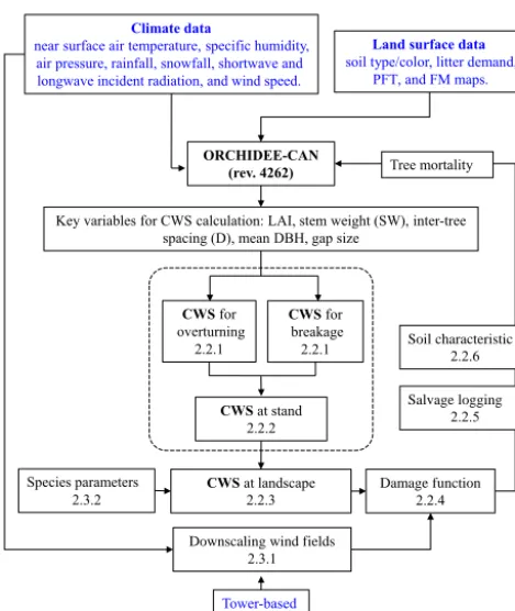
In ORCHIDEE-CAN (revision 4262) the biomass of the dif-ferent pools, leaf area index, crown volume, crown density, stem diameter, stem height, and stand density are simulated as the accumulated growth and are passed to the wind-throw module. The wind-throw module calculates the critical wind speed based on the principles applied in ForestGALES (Gar-diner et al., 2000) and storm damage based on the approach developed and tested by Anyomi et al. (2017). Figure 1 sum-marizes the major components of storm damage calculations in ORCHIDEE-CAN. A more detailed description of the dif-ferent components in the figure is presented in following sec-tions.
2.2.1 Critical wind speeds (ForestGALES)
The presence or absence of storm damage in a forest stand can be modelled with the concept of critical wind speed. If the wind speed exceeds the critical wind speed of a for-est, the forces applied by the wind speed are sufficient to overturn the whole tree or break its stem. The exact value of the critical wind speed depends on the canopy structure (Vollsinger et al., 2005; Hale et al., 2012), the tree species, the soil properties, and the root profiles (Nicoll et al., 2006). In this study, the physics formalized in ForestGALES (Gar-diner et al., 2010; Hale et al., 2015), a hybrid mechanistic for-est wind damage risk model, were added into ORCHIDEE-CAN (revision 4262) to simulate the critical wind speeds of all forest stands. The model simulates the critical wind speed for two types of damage: tree overturning and stem breakage. The critical wind speed for overturning is calculated as
CWSov=
1 κD
Creg·SW
ρGd
12
1 fCW·fedge
12
ln
h−d z0
, (1)
where CWS is the critical wind speed (m s−1), and the sub-script ov denotes the critical wind speed for overturning.κis von Karman constant and D is the inter-tree spacing (m).
tree-Climate data
near surface air temperature, specific humidity, air pressure, rainfall, snowfall, shortwave and longwave incident radiation, and wind speed.
Land surface data
soil type/color, litter demand, PFT, and FM maps.
ORCHIDEE-CAN (rev. 4262)
Key variables for CWS calculation: LAI, stem weight (SW), inter-tree spacing (D), mean DBH, gap size
Species parameters 2.3.2
CWSfor
overturning 2.2.1
CWSfor
breakage 2.2.1
CWS at stand 2.2.2
CWSat landscape
2.2.3 Damage function2.2.4
Downscaling wind fields 2.3.1
Tower-based wind speed
Tree mortality
Salvage logging 2.2.5 Soil characteristic
2.2.6
Figure 1.Information flow of this study showing the link between the different elements presented in Sects. 2.2 and 2.3 (numbers in the figure refer to section numbers in the text). The diagram shows input data in blue. The dashed box shows critical wind speed calcu-lations according to ForestGALES.
pulling experiments (N m kg−1; Nicoll et al., 2006). SW is the green weight of the bole of the tree (kg). SW is calculated by multiplying the model-simulated above-ground biomass with green density for different tree species (see Table 2).
fCW is the enhanced momentum caused by the overhanging
displaced mass of the canopy. In ORCHIDEE-CANfCWwas
set to 1.136 (unitless), as suggested by Nicoll et al. (2006) from analysing extensive tree-pulling data. In other words, the applied turning moment is a constant fraction of the to-tal turning moment. fedge is the edge factor (unitless) and
a detailed description of the factor is given in Sect. 2.2.2.
Gis the gust factor (unitless) and its calculation is also de-scribed in section Sect. 2.2.2; h is the average tree height (m), d is the zero-plane displacement (m),z0 is the
rough-ness length (m), and all are simulated by ORCHIDEE-CAN (Naudts et al., 2015). Note thatdandz0depend on the wind
speed at canopy heightuh, and hence iterations are required
to solve Eq. (1) (see below).
The critical wind speed for stem breakage is calculated as
CWSbk=
1
κD
π·MOR·dbh3
32ρG(d−1.3)
!12
fknot
fCW·fedge
12
ln
h−d
z0
, (2)
where the subscript bk denotes stem breakage, MOR is the modulus of rupture (Pa) of green wood and was parameter-ized for different tree species (see Table 2), and dbh (m) is the tree diameter at breast height as simulated by ORCHIDEE-CAN;fknot is a factor to reduce wood strength due to the
presence of knots (unitless). Similar to Eq. (1),d andz0in
Eq. (2) also depended on the wind speed measured at canopy heightuh, and hence iterations are required to solve Eq. (2)
(see below).
The relationships between the aerodynamic parameters (d
andz0) and the vegetation structure follow the analytical
re-lationships proposed by Raupach (1994):
d(uh)=h
1−
1−e−
cd1 C
w·Cd D2
C·u−hn
1 2
cd1
Cw·Cd
D2
C·u−hn
1 2
, (3)
z0(uh)=(h−d) (e−κ·γ+9h), (4)
wherecd1is a regression parameter (cd1=7.5),Cwis crown
width (m), and Cd is crown depth (m). Individual trees
in the model are simulated as spherical elements, and the canopy width and canopy depth are thus identical;γ is a parameter that depends on the canopy characteristics (γ=
1
(0.003+0.15·Cw·Cd D2 )
1/2,max(
Cw·Cd
D2 )=0.6), and9his the atmo-spheric stability correction function (9h=ln(2)−1+12).
Tree crowns, branches, and stems are considered as porous and flexible materials that will streamline and thus change their shape with changing wind speed (uh). Streamlining
was parameterized through the parametersC andn, which were reported for wind tunnel experiments with different tree species (Rudnicki et al., 2004; Vollsinger et al., 2005) (see Table 2). The maximum value ofCD=C·u−hn is set
at uh = 10 m s−1 and the minimum value of CD is set at
uh = 25 m s−1 (limits are based on wind speed range in
Mayhead, 1973). The species-specific streamlining effect for wind speeds outside of this range was calculated by holding
uhconstant to its lower or higher threshold. In other words,
CDwas implemented as a kind of step function.
Critical wind speeds are calculated as the solutions to a non-linear set of equations for overturning, i.e. Eqs. (1), (3), and (4), and another set of equations for stem breakage, i.e. Eqs. (2), (3), and (4). An initial wind speed,uh=25 m s−1,
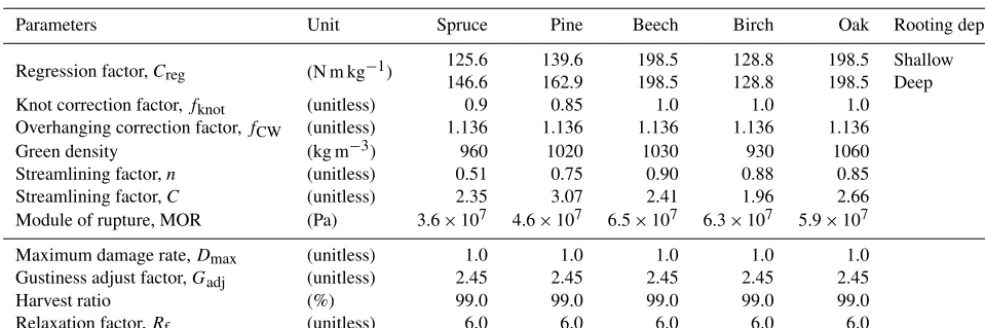
Table 2.Parameter values used in the ORCHIDEE-CAN wind-throw module. The scientific names of the tree species are given in Sect. 2.3.2.
Parameters Unit Spruce Pine Beech Birch Oak Rooting depth
Regression factor,Creg (N m kg−1) 125.6 139.6 198.5 128.8 198.5 Shallow
146.6 162.9 198.5 128.8 198.5 Deep
Knot correction factor,fknot (unitless) 0.9 0.85 1.0 1.0 1.0
Overhanging correction factor,fCW (unitless) 1.136 1.136 1.136 1.136 1.136
Green density (kg m−3) 960 1020 1030 930 1060
Streamlining factor,n (unitless) 0.51 0.75 0.90 0.88 0.85
Streamlining factor,C (unitless) 2.35 3.07 2.41 1.96 2.66
Module of rupture, MOR (Pa) 3.6×10⁷ 4.6×10⁷ 6.5×10⁷ 6.3×10⁷ 5.9×10⁷
Maximum damage rate,Dmax (unitless) 1.0 1.0 1.0 1.0 1.0
Gustiness adjust factor,Gadj (unitless) 2.45 2.45 2.45 2.45 2.45
Harvest ratio (%) 99.0 99.0 99.0 99.0 99.0
Relaxation factor,Rf (unitless) 6.0 6.0 6.0 6.0 6.0
of uh=25 m s−1, is applied to Eqs. (3) and (4) to obtain an
approximation for CWSbkby Eq. (2). Subsequently,uhis set
to the value of CWSov (or CWSbk) to estimate the
aerody-namic parameters (dandz0) for the next iteration. The
itera-tion process is stopped if the difference in CWS between two iterations falls below 0.01 m s−1or the number of iterations exceeds a threshold of 20.
Whereas ORCHIDEE-CAN is designed to simulate both even- and uneven-aged stands, ForestGALES is currently limited to simulating the critical wind speeds for even-aged forests. Although this difference in design is thought to have few consequences, it is considered essential in the calcula-tion of the ratio between tree height and tree spacing (the so-called inter-tree spacing,D). In an even-aged stand both tree spacing and tree height are homogeneous and thus well defined at the stand level. This is no longer the case for tree height in uneven-aged stands. This issue is accounted for by calculating a critical wind speed for each diameter class sep-arately. Although this approach addresses the possible het-erogeneity in tree height, it requires a value for inter-tree spacing, by definition a stand characteristic, to be calculated for each diameter class. To calculate the inter-tree spacing for each diameter class, firstly the total woody biomass at the stand level is calculated. Subsequently, this total woody biomass is divided by the biomass of the modelled trees in each diameter class. The outcome is considered the virtual inter-tree spacing of the diameter classD and was used in Eqs. (1) and (2) to calculate the critical wind speeds for each diameter class.
By default three diameter classes are used to describe the heterogeneity within a forest stand. ORCHIDEE-CAN then calculates the critical wind speed for breakage and overturn-ing based on the vegetation structure parameters for each di-ameter class. When using three didi-ameter classes, as is the case in this study, a total of six critical wind speeds are thus calculated for each forest in each grid box. Subsequently, the lowest critical wind speed is used to determine the
dam-age type for each diameter class. The number of damdam-aged trees in each diameter class is then calculated by multiplying the damage rate (Dβ; see Sect. 2.2.4) with the tree numbers
within each diameter class. The total number of trees dam-aged by a storm was calculated as the sum of the damdam-aged trees in each diameter class.
2.2.2 Gustiness and edge effect (ForestGALES)
ORCHIDEE-CAN is driven by half-hourly wind fields. For storm damage, such a time step is already too large because the half-hourly wind field hides the extreme wind gusts that occur within a half-hourly time step. Storm damage is deter-mined more by the extreme gusts than by the average wind speed. This scaling issue is dealt with by explicitly simu-lating the gustiness through the so-called gust factor. The gust factorGwas parameterized as a function of inter-tree spacing to tree height ratio and edge distance to the tree height ratio. These dependencies and their parameter values are based on wind tunnel experiments (Gardiner et al., 2000; Hale et al., 2012, 2015).
G=
−2.1·D
h +0.91
·x h
+
1.0611·ln
D
h
+4.2
·Gadj, (5)
where Dh is constrained between 0.075 and 0.45, and x is parameterized as a function of leaf area index (LAI), i.e.
x=28h
LAI for the inner area near recent gaps andx=9hfor
the outer area forest away from such gaps (see Sect. 2.2.3). The length scale parameterx was derived from large eddy simulation (Pan et al., 2014).Gadj is a linear scaling factor
by the model (see Fig. S1 in the Supplement). At the inner area, the effect of vegetation structure on wind speed is ac-counted for through the edge factorfedgein Eqs. (1) and (2).
The calculation of fedge follows the approach proposed by
Gardiner et al. (2000).
fedge=
(2.7193(Dh)−0.061)+(−1.273(Dh)+0.9701)
(0.68(Dh)−0.0385)+(−0.68(Dh)+0.4785)
·(1.1127(Dh)+0.0311)xh ·(1.7239(Dh)+0.0316)xh
(6)
At the outer area, the edge effect is negligible such thatfedge
is set to 1.0.
2.2.3 Vegetation structure
Vegetation structure is simulated at the landscape and the stand level (see Fig. 1). At the landscape level the simulations distinguish between forests with a newly formed forest edge and forest with established edges. Edges result from natural or anthropogenic stand-replacing disturbances. First, the sur-face area of stand-replacing disturbances is cumulated over the last 5 years (A5), a time horizon corresponding to the
time required for forests near newly formed edges to adapt to the increased gustiness (Gardiner and Stacey, 1996). By prescribing the average gap size (Agap) to 2 ha and
assum-ing gaps are square shaped and the gustiness is affected over a distance of 9 times the canopy height (9h) (Gardiner and Stacey, 1996), the forest area that experiences an increased gustiness due to proximity to recent gaps (Ainner) is
calcu-lated as
Ainner=
1 4·
A
1 2
gap+2·9h
2
−Agap
!
·
A5
Agap
, (7)
where the factor of14accounts for the fact that only the down-wind edge perpendicular to the down-wind will experience an in-creased gustiness. The second term is the inner area gener-ated by a single gap and the third term is the total number of gaps in the grid cell. The forest area that has no edges in its proximityAouteris calculated as the residual:
Aouter=
(
Agrid−(A5+Ainner), whenA5+Ainner< Agrid
0 andAinner=Agrid, whenA5+Ainner≥Agrid, (8)
whereAgridis the area of the grid box being modelled.
2.2.4 Storm damage
With wind speeds approaching the critical wind speed, dam-age such as defoliation and branch damdam-age become more likely. Once the wind speed exceeds the critical wind speed, overturning and stem breakage are possible but their likeli-hood increases with further increasing wind speeds. A sig-moid damage function is used to simulate the rate of storm
damage to a forest. A similar approach has been applied and tested by Anyomi et al. (2017) for estimating storm damage as a function of the daily maximum wind speed. This rela-tionship is formalized as
Dβ=Dmax
1
1+e−
Umax−CWSbk, ov Rf
−
1
1+e
CWSbk, ov Rf
, (9)
whereDβ is the damage rate (unitless) and thus the share of
trees that will be killed,Dmaxis an observed maximum
dam-age rate, which was set to 1.0,Rfis a relaxation parameter to
adjust the damage rate given by a certain wind speed below the model-calculated critical wind speed, and a value 6.0 was applied for all tree species.Umaxis the maximum daily wind
speed from the forcing or model calculation. Subsequently, the lowest out of the six calculated critical wind speeds (see Sect. 2.2.1) is used to determine the damage type for each di-ameter class. The number of damaged trees in each didi-ameter class is then calculated by multiplying the damage rate (Dβ)
with the tree numbers within each diameter class. The total number of trees damaged by a storm was calculated as the sum of the damaged trees in each diameter class.
2.2.5 Salvage logging
Damaged wood due to storms is often left on-site in un-managed forests; however, salvage logging is often carried out for a managed forest in order to recover some of the economic losses and avoid large-scale insect outbreaks trig-gered by wind disturbance. When dealing with the effects of wind damage on the biomass pools of forests, the anthro-pogenic response to storm damage needs to be accounted for. ORCHIDEE-CAN distinguishes managed and unmanaged forest. In unmanaged forests all carbon contained in trees killed by wind storms ends up in the litter pools. For man-aged forests, a prescribed harvest ratio determines the wood that is salvage logged and the wood left on-site. In species that are prone to bark beetle attacks following wind throw, the volume left on-site is very small. In Sweden, a maxi-mum volume of 5 m3ha−1of newly damaged logs is allowed.
However, following large-scale storm damage this threshold has been temporarily lowered to 3 m3ha−1in order to reduce the risk of spruce bark beetle outbreaks. Following Gudrun, it was observed that no more than 1.8 to 1.1 m3ha−1was left on-site. Given that the current implementation of storm dam-age was designed to deal with large wind storms, with a fair risk for subsequent bark beetle outbreaks (Kärvemo, 2015), applying a very high efficiency for salvage logging, i.e. 99 %, appears justified (Schroeder et al., 2006).
2.2.6 Soil characteristics
considers all soils to be free draining at the bottom of the soil layers. This assumption differs from ForestGALES in which four soil classes with different drainage are distinguished (Hale et al., 2015): freely draining mineral soil, gleyed (i.e. waterlogged and lacking in oxygen) mineral soil, peaty min-eral soil, and deep peat. At present, ORCHIDEE-CAN only uses the ForestGALES parameters for freely draining min-eral soils. Owing to this assumption ORCHIDEE-CAN is expected to overestimate the critical wind speed, resulting in less damage, for locations with shallow and/or wet soils.
Furthermore, ForestGALES distinguishes shallow-, medium-, and deep-rooting species. This classification was applied in ORCHIDEE-CAN through the parameter (humcte) describing the vertical root profile. In ORCHIDEE-CAN, the rooting density is assumed to following a function that decreases exponentially from the top to the bottom of the soil layers and is considered independent from site conditions or stand age. If 90 % of total root mass was found above a depth of 2 m, the species was considered shallow rooted. The effect of rooting depth on critical wind speeds was accounted for by using a different regressing coefficient
Creg for shallow- and deep-rooting species (see Table 2).
Under the current parameter settings of the rooting profile, ORCHIDEE-CAN considers all tree species to be shallow rooted. Note that in ORCHIDEE-CAN the rooting profile is also a critical parameter with which to calculate the drought stress of trees.
When the soil is frozen, ORCHIDEE-CAN only allows wind storm damage from stem breakage. In other words, there is no overturning of trees when the soil is frozen. The soil temperature at 0.8 m below the surface was used as the threshold to decide whether the soil was frozen or not.
2.3 Model parameterization 2.3.1 Downscaling wind fields
In this study, simulations are forced by 6 h CRU-NCEP cli-mate reanalysis (Viovy, 2011; Maignan et al., 2011). The ternal weather generator of the ORCHIDEE-CAN model in-terpolates this reanalysis to obtain the half-hourly (30 min) mean wind speed used in the calculation of storm damage. Interpolation of the 6 h reanalysis is expected to dampen the wind speed and therefore wind damage calculated by ORCHIDEE-CAN would be underestimated. To overcome this issue a tuning parameter called mean wind ratio (MWR) was introduced.
The MWR converts the mean wind speed from 6 h CRU-NCEP reanalysis into a mean wind speed at the 30 min time step. ORCHIDEE-CAN then uses these daily maximum es-timated values to calculate damage rates that may occur in a forest stand near or away from forest edges. Note that in this study the values for the mean wind ratio are specific for the CRU-NCEP half-degree forcing at a 6 h time step. The mean
wind ratio will thus need to be re-parameterized if the wind driver is replaced by any other forcing.
The MWR was estimated from 38 European eddy-covariance sites covered by forests for which the meteorolog-ical data were freely available. For the period 1996 to 2007, 208 site–year combinations were retained for which over 60 % of the half-hourly measurements were available. The remaining data gaps were filled with the ERA-Interim reanal-ysis data (Dee et al., 2011; Vuichard and Papale, 2015). The 208 site–years were extracted from the CRU-NCEP reanal-ysis. Subsequently, the ratio between the maximum 30 min mean wind speed within a 6 h period and the 6 h mean wind speed obtained for the same location and time frame from the CRU-NCEP reanalysis was calculated.
MWR= UFluxnet UCRU-NCEP
, (10)
where the subscripts Fluxnet and CRU-NCEP denote the data source,UFluxnet is the maximum value of the 30 min mean
wind speeds (m s−1) within a 6 h time frame, andUCRU-NCEP
is the 6 h mean wind speed from the CRU-NCEP dataset. Fi-nally, maximum wind speeds in the time series of each forest site were stratified according to the wind force catalogue in Beaufort wind scale (BWS), an empirical measure that re-lates wind speed to observed conditions on land (National Meteorological Library and Archive, 2010). Data were then analysed to account for the relationship between the mean wind speed and the ratio between the observed and temporal average mean wind speed.
The quality of the fitted relationship was calculated as the root mean square error (RMSE). RMSE is a statistic that is widely applied to quantify the difference between values pre-dicted by a model and the values actually observed:
RMSE=
q
[mean(Yi−Fi)]2, (11)
whereY denotes the observed values, F denotes the mod-elled values, and the subscription i is the sample index. RMSE is used throughout this study to quantify the good-ness of fit between observed and predicted values.
2.3.2 Critical wind speeds for five tree species
The calculation of critical wind speeds is parameterized for five common tree species in Europe: Norway spruce (Picea
sp.), Scots pine (Pinus sylvestris), beech (Fagus sylvatica), birch (Betulasp.) and oak (Quercus ilexandQuercus suber). In ORCHIDEE-CAN these five tree species are simulated as separate PFTs over Europe. Parameters for the other PFTs within and outside of Europe were based on ForestGALES, which has been parameterized for 21 tree species including the five species simulated by ORCHIDEE-CAN. Table 2 lists the parameters used in ORCHIDEE-CAN to calculate the critical wind speeds.
species in Les Landes. These regions were only used to test the model. The anticipated simulation domain of this new development is Europe. The five species for which the model was tested make up 67 % of the European forest cover. In terms of taxonomic families the representativeness increases to>90 % (Koeble and Seufert, 2001).
3 Observational data, model tuning, and evaluation 3.1 Storm damage observations
A 60-year-long record of storm damage statistics over Swe-den was extracted from the country-level European Forest Institute storm damage database from 1951 to 2010 (Nilsson et al., 2004; Schlyter et al., 2006; Bengtsson and Nilsson, 2007; Gardiner et al., 2010). We refined this dataset with re-gional information. Following Gudrun in January 2005, the Swedish Forest Agency mapped the spatial distribution of the storm damage for damage classes ranging from 5 to 50 m3 per ha in steps of 5 m3for the first damage class and 10 m3 for all subsequent classes (see Fig. 7). The storm made land-fall near the south of Norway, went through the north of Gö-taland, and resulted in extensive forest damage in the central area of Götaland. The area around the cites of Ljungby and Växjö was reported as having the greatest damage of about 30 m3ha−1. The spatial extent of storm damage was retrieved from ocular inspection of aircraft images processed by the Swedish Forest Agency. In January 2009, Klaus made land-fall in south-western France near Les Landes forest and dam-aged 43.1×10⁶m3of wood in France. The dynamics of sur-face albedo and LAI between 2001 and 2010 were extracted from MODIS and SPOT-VGT satellite images, receptively (Planque et al., 2017). These remote sensing time series were overlaid by ORCHIDEE-CAN simulations and compared at two locations between 2001 and 2010, thus resulting in a to-tal of 20 data points (shown as pink arrows in Fig. S2). 3.2 Model tuning for storm damage
Although all parts of the wind-throw module come with their own assumptions, parameters, and subsequent uncertainties, the calculation of the gustiness (G; Eq. 5) is considered to be among the most uncertain part of the model because it in-volves spatial and temporal scaling issues in both the driver data and the model formulation. Furthermore, the function that was used to convert the difference between the critical wind speed and wind speed into a damage rate (Dβ; Eq. 9)
is also thought of as very uncertain. The key parameters in these functions,GadjandRf, are empirical, lack a good
ob-servational constraint, and are therefore prime parameters to be tuned for matching the observations.
Given the availability of 60 years of observations of pri-mary damage caused by wind storms between 1951 and 2010 for the region (Gardiner et al., 2010), southern Sweden was selected as the study area for model tuning. Tuning made use
of the observed damage volumes for the years 1981 to 2000 because it is the most recent period without major storms. The storm Gudrun (2005) was deliberately excluded from the tuning period so it could be used as an evaluation of model performance.
The simulations used for parameter tuning started in 1981 and therefore had to be forced by a spatially explicit descrip-tion of the biomass distribudescrip-tion in southern Sweden at the end of the year 1980. In this study, the spatially explicit biomass distribution for 1980 was extracted from a previous study that simulated the effects of forest management and land cover changes in Europe between 1750 and 2010 (McGrath et al., 2015; Naudts et al., 2016). The previous study did not, however, account for the effects of wind storms on woody biomass and is therefore likely to overestimate the biomass in regions with chronic wind stress. This issue was overcome by starting the simulation in 1971 rather than 1981 and by running ORCHIDEE-CAN with the storm damage module between 1971 and 1980 to adjust the biomass to chronic wind stress. Chronic wind stress occurred mainly in western Nor-way. Subsequently, this adjusted spatially explicit descrip-tion of the biomass distribudescrip-tion was used in the simuladescrip-tions for parameter tuning. Trail-and-error tuning started on 1 Jan-uary 1981 and continued until 31 December 2000 by forcing the model with the CRU-NCEP reanalysis to simulate the primary damage caused by storm events including the 1999 Anatol storm.
3.3 Critical wind speeds for five tree species
Model implementation and parameterization were tested for all five tree species shared between ForestGALES and CAN (see Sect. 2.3.2) by running ORCHIDEE-CAN for a test pixel. The Fontainebleau forest, which is the closest large forest to the LSCE research institute, was arbi-trary selected as the simulation site and ORCHIDEE-CAN was run for 200 years by cycling over the CRU-NCEP re-analysis data from 1901 to 1930. Subsequently, the canopy structure variables simulated by ORCHIDEE-CAN, includ-ingh,D,Cw,Cd, and LAI, were used as the input data for a
stand-alone version of ForestGALES (MathCAD version) to estimate the CWSovand CWSbk. In total four types of CWSs,
CWSovand CWSbkfor the inner and outer forest, were
sim-ulated by both models for the same canopy structure. 3.4 Critical wind speeds over southern Scandinavia Southern Scandinavia was simulated as a 35 by 35 half-degree pixel grid. For each pixel, four critical wind speeds, i.e. CWSov and CWSbk for the inner and outer area of the
● ●
● ● ●
● ● ●
● ●
●
5 10 15 20
0
2
4
6
8
● ● ● ● ● ●
● ●
●
RMSE: 0.48 (CRU−NCEP, spatial−temporal aggregation) RMSE: 0.19 (Fluxnet, temporal aggregation)
Me
an
w
in
d
ra
tio
, M
W
R
(
un
itl
es
s)
6 h CRU−NCEP reanalysis, 6 h Fluxnet wind speed (m s )−1
BWS 1 BWS 2
BWS 3
BWS 4 BWS 5 BWS 6 BWS 7 BWS 8
BWS 9 BWS 10
BWS.11
Figure 2. Distribution of the mean wind ratio (MWR) in each Beaufort wind scale (BWS) and the relationship between the 6 h CRU-NCEP reanalysis wind speed and MWR. The fitting of the relationship (red line) used Eq. (12) with regression coefficients a0= −5.299,a1=2.051,a2= −0.191, anda3=0.006. This re-lationship is used to convert CRU-NCEP 6 h mean wind speed to the 30 min maximum wind speed in this study. The RMSE using this regression model to predict the mean value of MWR in each BWS class is 0.48. The open circles (grey colour) show the effect of 6 h temporal aggregation on the MWR from the selected Fluxnet sites in European forest. The grey line is the fitting line of the open circles.
as derived during the tuning phase. The model was restarted from the time point 31 December 2010 of the aforementioned simulation of Naudts et al. (2016), in which forest manage-ment and land use were prescribed from the historical recon-structions presented in McGrath et al. (2016). The vegetation over this area mainly consists of coniferous tree species, i.e. Norway spruce (Picea abies(L.) Karst) and Scots pine ( Pi-nus sylvestrisL.); however, a species mixture of coniferous tree and broadleaved species such as birch (Betula pendula
Roth and B. pubescens Ehrh.) can be found in this region (Drössler, 2010). The simulated spatial distribution of criti-cal wind speeds for each tree species thus reflects the effects on critical wind speeds of age class structure, forest manage-ment, and, to a lesser extent, local climate conditions. 3.5 Storm damage over Sweden
The capability of ORCHIDEE-CAN to simulate storm dam-age was evaluated by comparing the observed and simulated storm damage over Sweden from 1951 to 1980 and from 2001 to 2010. A simulation over Sweden was set up by using the CRU-NCEP reanalysis over the last half-century making
use of the parameter values forGadjandRfas derived during
the tuning phase. The region under study entails a 15 by 15 half-degree pixel grid covering southern Sweden and a sec-tion of Norway. The state of the forest in Sweden on 31 De-cember 1940 was described by using the matching year from an existing 250-year-long simulation (see also Sect. 3.2). Be-cause the 250-year-long simulation did not account for the effects of wind damage, the first 10 years from 1941 to 1950 of the simulation experiment were intended to reach equilib-rium between the vegetation and the mean wind speed. For these 10 years the climate data for 1941 to 1950 were used. Within the study domain, this approaches reduced the stand-ing biomass mainly in western Norway (not shown). Sub-sequently, the simulation experiment continued from 1951 to 2010, the period for which damage reports are available (Nilsson et al., 2004; Schlyter et al., 2006; Bengtsson and Nilsson, 2007; Gardiner et al., 2010). The years 1981 to 2000, which were used for parameter tuning, were excluded from the evaluation.
● ● ●
● ● ● ● ● ● ●●● ● ● ●
8 10 12 14 0 20 40 60 80 100 120
Tree height, spruce (m)
Cr
itical wind speed (m s
−1
) (a)
● ORCHIDEEov
ORCHIDEEbk ForestGALESov ForestGALESbk
RMSE,ov: 0.893 RMSE,bk: 1.29
● ● ● ● ● ● ● ● ● ●●● ● ●●
8 10 12 14 0 20 40 60 80 100 120
Tree height, spruce (m)
Cr
itical wind speed (m s
−1
) (f)
RMSE,ov: 1.44 RMSE,bk: 1.09
● ● ●● ● ●● ● ●● ● ●● ● ●
8 10 12 14 0 20 40 60 80 100 120
Tree height, pine (m) (b)
RMSE,ov: 1.000 RMSE,bk: 0.634
● ● ●● ● ● ● ●● ● ●● ● ●●
8 10 12 14 0 20 40 60 80 100 120
Tree height, pine (m) (g)
RMSE,ov: 0.345 RMSE,bk: 0.664
● ● ●●●●● ● ●● ● ●● ●●
8 10 12 14 0 20 40 60 80 100 120
Tree height, beech (m) (c) RMSE,ov: 0.722 RMSE,bk: 0.757 ● ● ●●●●● ● ●●●● ●●●
8 10 12 14 0 20 40 60 80 100 120
Tree height, beech (m) (h)
RMSE,ov: 0.579 RMSE,bk: 0.789
● ●● ●● ● ●●●●● ● ● ●●
8 10 12 14 0 20 40 60 80 100 120
Tree height, birch (m) (d) RMSE,ov: 0.413 RMSE,bk: 0.796 ● ●● ● ● ● ● ●● ●● ●● ●●
8 10 12 14 0 20 40 60 80 100 120
Tree height, birch (m) (i) RMSE,ov: 1.363 RMSE,bk: 1.252 ●●●● ●●●●●● ●●●● ●● ●●●● ●●●● ●●●● ●
8 10 12 14 0 20 40 60 80 100 120
Tree height, oak (m) (e) RMSE,ov: 1.477 RMSE,bk: 1.965 ●●●●●●●●● ●●●●●● ●●●● ●●●●●● ●●●●
8 10 12 14 0 20 40 60 80 100 120
Tree height, oak (m) (j)
RMSE,ov: 0.701 RMSE,bk: 0.985
Figure 3.Model-calculated critical wind speeds as a function of tree height for five common tree species in Europe. For each tree species the critical wind speed is calculated for overturning and stem breakage for forest located away from a forest edge (outer,a–e) and near a forest edge (inner,f–j). The ORCHIDEE-CAN simulations are shown as symbols and benchmarked against the ForestGALES simulations, which are shown as lines. The scientific names of the tree species are given in Sect. 2.2.3. The CWS differences between the ORCHIDEE-CAN and ForestGALES calculation were calculated using Eq. (11), for which the CWSs from ForestGALES were treated as the reference.
4 Results
4.1 Downscaling wind fields
The effect of spatial and temporal aggregation on wind fields can be found by the comparison of CRU-NCEP 6 h mean wind speed to the stand-level 30 min maximum wind speed. Due to spatial and temporal aggregation, the CRU-NCEP 6 h mean wind speed reanalysis consistently underestimates the 30 min maximal wind speeds. Stratification by the Beaufort wind scale revealed a clear relationship between this scale and the mean wind ratio for different Beaufort values (see Fig. 2). The low value of 6 h CRU-NCEP wind speed in the BWS10 bin may be due to the fact that all observations in this bin come from a single location wind category (Fig. S3). A fourth-order polynomial function was fitted through the observed MWR to downscale the CRU-NCEP 6 h mean wind speed to a max value of 30 min mean wind speed within a 6 h time frame.
Umax=a0UCRU-NCEP+a1UCRU-NCEP2 +a2UCRU-NCEP3
+a3UCRU-NCEP4 , (12)
where Umax is the max value of 30 min mean wind speed
(m s−1) within a 6 h period;a0toa3are regression
param-eters, which have the following values:a0= −5.299,a1=
2.051,a2= −0.191, anda3=0.006.
Given the intended use of this analysis to convert the 6 h mean wind speed of the CRU-NCEP reanalysis into a likely wind speed used by ORCHIDEE-CAN on the half-hourly timescale, the mean ratios of the maximum wind speeds were extracted for each Beaufort wind scale for a 6 h averaging pe-riod. The value of MWR for a 6 h averaging period increased from 1.0 to 6.0 when the Beaufort wind scale went up from scale 1 to scale 11.
4.2 Critical wind speeds for five tree species
Figure 4.The ORCHIDEE-CAN-calculated lowest critical wind speeds for overturning or stem breakage for forest located near (inner) and away (outer) from a forest edge. When making the display, the critical wind speeds from the three diameter classes and four age groups from
Piceaspecies were assessed and the lowest value was compared against the daily maximum wind speed for estimating the damage due to
storms. Lowest critical wind speeds in the forest away from a forest edge (outer)(a), lowest critical wind speeds in the forest near a forest edge (inner)(b), lowest critical wind speeds overlaid with the difference between maximum daily wind speed and lowest critical wind speed in outer area on 9 January 2005(c), and lowest critical wind speeds overlaid with the difference between maximum daily wind speed and lowest critical wind speed in the outer area(d). The contours show the positive wind speed difference in black and the negative wind speed difference in red. Forests within the red contours are expected to suffer from storm damage.
matched. The difference in CWSs from the two models (RMSE for all CWSs) was limited to a few metres per sec-ond ranging from 0.4 to 2.0 for different tree species. More-over, the estimates show that the critical wind speed close to a forest edge is always lower than the respective value further away from a forest edge. (e.g. Fig. 3f<a, ..., Fig. 3j<Fig. e). Also note that for oak, for example, the critical wind speeds for breakage and overturning are almost identical for small trees, but the difference between both critical wind speeds increases with increasing tree height (Fig. 3e and j). This implies that taller oak stands are more vulnerable to tree overturning than to stem breakage compared to smaller stands. The relationship between tree height and critical wind speed for spruce is very different compared to oak. For spruce the critical wind speeds for breakage and overturn-ing are within several m s−1 from each other and this dif-ference remains more or less constant with increasing tree height (Fig. 3a and f). In other words, both stem breakage
and tree overturning may occur simultaneously in tall spruce stands. Furthermore, small beech stands are more vulnerable to breakage (similar to spruce) but tall beech stands are more vulnerable to turnover (similar to oak; Fig. 3c and h).
● ● ● ● ● ● ● ● ● ● ● ● ● ● ● ● ● ● ● ●
1981 1982 1983 1984 1985 1986 1987 1988 1989 1990 1991 1992 1993 1994 1995 1996 1997 1998 1999 2000 ● ● ● ● ● ● ● ● ● ● ● ● ● ● ● ● ● ● ● ● 0 10 20 30 40 D am ag ed w oo d vo lu m e ( x 10 m ) 6
3 ● Reported
Rf =1.0, Gadj =1.0, RMSE=2.130
Rf =1.0, Gadj =3.0, RMSE=10.078
Rf =10., Gadj =3.0, RMSE=6.426
Rf =1.0, Gadj =2.45, RMSE=1.817
Rf =6.0, Gadj =2.45, RMSE=1.351
(a) ● ● ● ● ● ● ● ● ● ● ● ● ● ● ● ● ● ● ● ●
1981 1982 1983 1984 1985 1986 1987 1988 1989 1990 1991 1992 1993 1994 1995 1996 1997 1998 1999 2000
−2 −1 0 1 2 R el at iv e er ro r ( x 10 0 % ) (b)
Figure 5. Sensitivity of the simulated storm damage over Swe-den between 1981 and 2000 for different values for the relax-ation parameter (Rf) and the gust factor adjustment Gadj (a). Observed storm damage is extracted from Nilsson et al. (2004), Schlyter et al. (2006), Bengtsson and Nilsson (2007), and Gardiner et al. (2010). The relative model simulation error (calculated as (estimation−observation)/estimation) for the best-tuned case(b).
sustain wind speeds exceeding 40 m s−1. The proximity of forest edges is expected to decrease the critical wind speeds (Eqs. 1, 2, and 6). Indeed, a spruce forest close to a forest edge can sustain wind speeds ranging from 10 to 35 m s−1.
As already shown in Fig. 3a and f, the difference in criti-cal wind speeds between overturning and breakage are very small for spruce. This behaviour is sustained over a large spa-tial domain (compare Fig. 4a and b). We further compare the difference between these CWS maximum daily wind speeds on 9 January 2005. Forests located in the centre of southern Sweden are expected to suffer from storm damage for the Gudrun case (see Fig. 4c, d)
4.4 Storm damage over Sweden
The frequency of storm events in the period from 1981 to 2000 used for parameter tuning is about one storm every 5 to 10 years. The observed primary damage of these storms ranges between 2 and 5×10⁶m3 of wood (black line in Fig. 5). The sensitivity of the simulated damage for different values of the relaxation parameter Rf is presented in Fig. 5
(grey lines). Using the prior setting, i.e.Gadj=1 andRf=1,
results in an error (RMSE; Hyndman and Koehler, 2006)
1951 1954 1957 1960 1963 1966 1969 1972 1975 1978 1981 1984 1987 1990 1993 1996 1999 2002 2005 2008 ● ● ● ● ● ● ● ● ● ● ● ● ● ● ● ● ● ● ● ●●●●● ● ● ●●● ● ● ● ● ● ● ● ●●● ● ●● ● ● ● ● ● ● ● ●● ● ●● ● ● ● ● ● ● 0 20 40 60 80 D am ag ed w oo d vo lu m e ( x 1 0 m ) 6 3 (a) ● OBS SIM
1951 1954 1957 1960 1963 1966 1969 1972 1975 1978 1981 1984 1987 1990 1993 1996 1999 2002 2005 2008 ● ● ● ● ● ● ● ● ● ● ● ● ● ● ● ● ● ● ● ● ● ●●● ● ● ● ● ● ● ● ●● ● ● ● ● ●● ●● ● ● ● ● ● ● ● ● ● ●● ● ● ● ● ● ● ● ● −2 −1 0 1 2 R el at iv e er ro r ( x 10 0 % ) (b)
Figure 6. Comparison of the storm damage simulated by the ORCHIDEE-CAN and the reported wood damage over Sweden from 1951 to 2010. Observed storm damage is extracted from Nils-son et al. (2004), Schlyter et al. (2006), BengtsNils-son and NilsNils-son (2007), and Gardiner et al. (2010). The dashed-line area is the pe-riod from 1981 to 2000, which was selected for parameterization. The RMSE of the estimated storm damage is 1.35×10⁶m3 for the parameterization period and 5.05×10⁶m3during the evalua-tion period. The validaevalua-tion period ranges from 1951 to 2010 but ex-cludes the years 1981 to 2000. The relative model simulation error for the validation period from 1981 to 2010(b).
of about 2×10⁶m3 for a calibration period without major storms. Higher parameter values, e.g.Gadj=3.0, make the
model overestimate storm damage by up to 10×106m3. Pa-rameter tuning (Gadj=2.45 andRf=6.0) resulted in a
mod-est reduction of the deviation between observations and sim-ulations, i.e. an RMSE of 1.35×10⁶m3, and was therefore used to evaluate the wind-throw model.
The RMSE was largely determined by the simulated dam-age for 1986, 1987, and 2000. For these years, no damdam-age above the background volume was observed despite the pres-ence of high wind speeds in the CRU-NCEP reanalysis over southern Sweden in December and January for those three years. Regardless of the value used for Rf, the high wind
speeds in the CRU-NCEP reanalysis resulted in substantial damage volumes compared to the observations. This result suggests that ORCHIDEE-CAN would benefit more from improving the representation of gustinessGadjthan from
Figure 7.The case study of the storm Edwin (Gudrun) on 8 Jan-uary 2005. The colour scale shows the damaged woody volume (m3ha−1) due to this event.
The forest extent has expanded strongly in southern Swe-den during the 20th century. In 1940 the forestry system was different from that of today. The clear-felling system that pro-duces the forest edges modelled in this study was not widely adopted until the 1950s. This means that the state of the forest and the exposure to strong wind was very different in the be-ginning and at the end of the simulation period. ORCHIDEE-CAN partly simulates this transition: in 1940 the average simulated above-ground biomass was 154 m3ha−1, while in 1990 the biomass had increased to 168 m3ha−1. Within this half-century the simulated forest area in Sweden in-creased from 242 500 to 247 100 km2and the share of high stand management increased from 54.8 to 69.2 %. Despite ORCHIDEE-CAN accounting for the observed forest tran-sition, the model mostly underestimated the damaged wood volumes of large storms.
In January 2005, Gudrun caused the biggest recorded storm damage in Swedish history. We extracted the simula-tion result from the evaluasimula-tion experiment and calculated the total simulated storm damage by Gudrun. Simulated storm damage was 76.6×10⁶m3, which compares well to the re-ported 75.0×10⁶m3(Gardiner et al., 2010). Moreover, the high-level damage pixels (>30 m3per ha) are located in cen-tral Götaland, which demonstrates that when the driver data locate the storm in the right location, the model has the capa-bility to reproduce the spatial distribution for the event (see Fig. 8).
The model, however, underestimated the storm damage in 2007 (Fig. 5). Given the reconstructed wind speed in the driver data, the observed storm damage appears high. The failure of the model to simulate the right order of magnitude in storm damage in 2007 may be for two reasons: (1) the CRU-NCEP reconstruction underestimated the wind speed and/or (2) ORCHIDEE-CAN overestimated the critical wind speed by not accounting for the legacy effects of Gudrun,
Figure 8.Simulated spatial distribution of the damaged wood vol-ume (m3ha−1) over southern Sweden by Gudrun in January 2005.
such as decreased tree stability owing to root damage or in-creased gap sizes following Gudrun. Additionally, the ob-served storm damage is more uncertain than for Gudrun be-cause the inventory in 2007 was not made as detailed as for Gudrun.
4.5 Biophysical effects of storms
5 Discussion
5.1 Downscaling wind fields
Wind is a highly heterogeneous turbulent flow of air. The flow consists of various sized eddies, and because the energy is conserved, changes in the distribution of the eddy size will result in different flow regimes. Gusts are generated when the flow passes over a heterogeneous surface such as val-leys, ridges, objects, or any surface warmer or cooler than its surroundings (Lanquaye-Opoku and Mitchell, 2005; Liu and Weng, 2009). The temporal resolution of a gust is seconds to minutes and its spatial resolution is metres. The highest wind speeds are caused by these gusts and are responsible for most of the storm damage (Usbeck et al., 2010).
The success of a large-scale model in simulating storm damage will thus to a large extent depend on the capability of the model to simulate gusts. At present, large eddy simu-lations are the most advanced approach to simulate the tur-bulent flow of air (Moeng, 1984; Dupont and Brunet, 2008). The high computational demand of the method (Yang, 2015) currently prevents it from being used in large-scale models such as ORCHIDEE-CAN. Likewise, advances in regional atmospheric modelling resulted in the capacity to simulate gusts and gust gradients in the wind field such as tornados (Ishihara et al., 2011) and hurricanes (Vickery et al., 2009). The computational requirements of regional models is also too high to consider them for global simulations. High com-putational needs can be avoided by using statistical down-scaling but these methods come at the expense of a poor pro-cess representation (Larsén and Mann, 2006; Salameh et al., 2009; Huang et al., 2015; Winstral et al., 2017). Moreover, the statistical relationship used for downscaling the gridded wind field from a coarse to a fine resolution depends on the gridded wind field and its spatial and temporal resolutions.
In this study, we used a statistical approach that builds on the relationship between in situ observations and the grid-ded reanalysis data. The simplicity of the approach enabled us to focus on implementing, developing, and validating the storm damage model rather than improving the physical rep-resentation of gusts in ORCHIDEE-CAN. Downscaling the gridded wind field from a coarse resolution to a fine reso-lution requires accounting for both spatial and temporal ag-gregation. Our approach made use of the mean wind ratio to convert the mean wind speed from 6 h CRU-NCEP reanaly-sis into a mean wind speed at the 30 min time step. By fur-ther analysing the contribution of spatial and temporal ag-gregation to downscaling (see Fig. S3), it was found that the temporal averaging was responsible for about 40 % of the reduction of the variation, whereas spatial averaging was re-sponsible for the remaining 60 %. In other words, simulating storm damage in large-scale models would initially benefit most from increasing the spatial resolution as that would al-low us to better account for the extreme wind speeds.
Note that in ORCHIDEE-CAN (revision 4262) the down-scaled wind speed is only used to test whether the critical wind speed is exceeded and, if so, to simulate the result-ing damage from stem break and overturnresult-ing. Consequently, the downscaled wind speeds are not used for calculating sur-face roughness, momentum, heat exchange, and water vapour transfer. The current statistical downscaling is thus not suit-able for use in model set-ups in which ORCHIDEE-CAN is coupled to an atmospheric circulation model, for exam-ple, LMDZ (Hourdin et al., 2006). Simulating storm dam-age from coupled land–atmosphere models, e.g. LMDZ– ORCHIDEE-CAN, will thus require an effort to better repre-sent turbulent air flow in the planetary boundary layer. 5.2 Storm damage over Sweden
The state of the forest in Sweden on 31 December 1940 was described by using the matching year from an existing sim-ulation, which ran from 1750 to 2010 (Naudts et al., 2016). This existing simulation accounted for land cover changes and changes in forest management following the histori-cal reconstruction of forest cover and management by Mc-Grath et al. (2015), but it did not account for storm damage. However, the forest reconstruction map shows that the forest species over Sweden mainly consist of Scots pine, Norway spruce, and birch, which is comparable with the report made by Helmfrid (1991).
Given its strength, the 1999 storm Anatol resulted in rel-atively little damage (5×10⁶m3), likely because it hit the southernmost part of Sweden where the landscape contains fewer forests and the share of broadleaf forest is much higher than just a few tens of kilometres north of the storm track. Although the good match between the data and the model (Fig. 5) is due to the fact that Anatol occurred within the tuning period, the conditions that are held responsible for the low volume of storm damage were indeed found to be reproduced. The CRU-NCEP reanalysis suggests the Anatol storm track hitting southern Sweden, and ORCHIDEE-CAN uses a forest index of 56 % in the storm track, but 68 % for landscapes 100 km north of the track. Furthermore, in 1999, 67 % of the simulated forests were broadleaved in southern Sweden, whereas roughly one-third were 100 km north of the track. Finally, ORCHIDEE-CAN simulates higher crit-ical wind speeds for broadleaved trees (especially in winter) than for conifers (Fig. 4).
● ●
● ●
● ●
● ●
● ●
●●
● ●
● ●
● ●
● ●
0.020 0.025 0.030 0.035 0.040
0.04 0.05 0.06 0.07 0.08 0.09 0.10
Visible albedo, MODIS (−)
Visib
le albedo
, ORCHIDEE (−)
(a) ●
●
Before storm Klaus (2009) After storm Klaus (2009)
● ●
● ●
● ●
● ●
● ●
● ●
● ●
● ●
● ●
● ●
1.5 2.0 2.5 3.0 3.5 4.0 4.5 5.0
1.5 2.0 2.5 3.0 3.5 4.0 4.5
LAI, SPOT−VGT (−)
LAI, ORCHIDEE (−)
(b)
●
● ●
● ●
● ●
●
● ●
Jun−01 Jun−02 Jun−03 Jun−04 Jun−05 Jun−06 Jun−07 Jun−08 Jun−09 Jun−10 0.06
0.08 0.10 0.12 0.14 0.16 0.18 0.20
Date (−)
Surf
ace roughness (m)
(c)
● ● ● ● ● ● ●
●
● ●
Jun−01 Jun−02 Jun−03 Jun−04 Jun−05 Jun−06 Jun−07 Jun−08 Jun−09 Jun−10 0.5
1.0 1.5 2.0 2.5 3.0 3.5
Date (−)
Tr
an
sp
ira
tio
n
(m
m
d
ay
)
(d)
-1
Figure 9. Effects of the wind storm Klaus (January 2009) on the forest in Les Landes, France. Comparison of the ORCHIDEE-CAN-simulated visible albedo and the MODIS observations in summertime (June) from 2001 to 2010(a). Comparison of the ORCHIDEE-CAN-simulated leaf area index (LAI) and SPOT-VGT-derived estimates in summertime (June) from 2001 to 2010(b). The dynamics of roughness for the most damaged pixel in Les Landes forest simulated by ORCHIDEE-CAN on a monthly timescale from 2001 to 2010 (c). The summertime (June) transpiration rate for the most damaged pixel in Les Landes forest simulated by ORCHIDEE-CAN(d). The shading indicates the period after the passing of Klaus in January 2009.
in the calculation of the RMSE, the model errors decrease to 1.62×10⁶m3(see Fig. 6). The RMSE is thus largely due to underestimating the damage during big storms.
5.3 Subpixel heterogeneity
Gusts and thus storm damage are often generated by surface heterogeneities, for example, forest edges, surface topogra-phy, and landscape features, with a very different tempera-ture than the surrounding landscape. Whereas these hetero-geneities can be accounted for in large eddy simulations and regional models, large-scale models such as ORCHIDEE-CAN managed to limit their computational costs by, among other simplifications, ignoring these subpixel heterogeneities (Krinner et al., 2005). When implementing processes that are partly driven by these heterogeneities, i.e. storm damage, these models are thus operated at the limit of their design. In this study, we have tried to overcome this issue by recon-structing subpixel heterogeneity from the wood harvest
ag-gregated over the last 5 years and assuming that all gaps are square-shaped and have a surface area of 2 ha (see Eqs. 7–8). This approach enabled ORCHIDEE-CAN to calculate sep-arate critical wind speeds for forest close to a forest edge (inner) and forests away from a forest gap (outer).