https://doi.org/10.5194/gmd-11-561-2018 © Author(s) 2018. This work is distributed under the Creative Commons Attribution 4.0 License.
BEATBOX v1.0: Background Error Analysis Testbed
with Box Models
Christoph Knote1, Jérôme Barré2, and Max Eckl1,a
1Meteorological Institute, LMU, 80333 Munich, Germany
2European Centre for Medium-Range Weather Forecasts, Shinfield Park, Reading, RG2 9AX, UK anow at: Institute of Atmospheric Physics, DLR, 82234 Oberpfaffenhofen, Germany
Correspondence:Christoph Knote ([email protected]) and Jérôme Barré ([email protected]) Received: 12 August 2017 – Discussion started: 4 October 2017
Revised: 19 December 2017 – Accepted: 2 January 2018 – Published: 8 February 2018
Abstract. The Background Error Analysis Testbed (BEAT-BOX) is a new data assimilation framework for box mod-els. Based on the BOX Model eXtension (BOXMOX) to the Kinetic Pre-Processor (KPP), this framework allows users to conduct performance evaluations of data assimilation experi-ments, sensitivity analyses, and detailed chemical scheme di-agnostics from an observation simulation system experiment (OSSE) point of view. The BEATBOX framework incorpo-rates an observation simulator and a data assimilation system with the possibility of choosing ensemble, adjoint, or com-bined sensitivities. A user-friendly, Python-based interface allows for the tuning of many parameters for atmospheric chemistry and data assimilation research as well as for educa-tional purposes, for example observation error, model covari-ances, ensemble size, perturbation distribution in the initial conditions, and so on. In this work, the testbed is described and two case studies are presented to illustrate the design of a typical OSSE experiment, data assimilation experiments, a sensitivity analysis, and a method for diagnosing model er-rors. BEATBOX is released as an open source tool for the atmospheric chemistry and data assimilation communities.
1 Introduction
Current regional and global models of the composition of Earth’s atmosphere exhibit a high level of complexity due to the combination of chemical and meteorological processes such as transport, thermodynamics, radiation, or precipita-tion. But “just” gas-phase chemistry itself already has a con-siderable amount of complexity. The number of variables
(chemical compounds) and equations (chemical reactions) in current model representations of tropospheric chemistry (“mechanisms”) can vary by 2 orders of magnitude (from 102to 104). Compare, for example, two well-known mecha-nisms: the Model for Ozone And Related Chemical Tracers version T1 (MOZART-T1; Emmons et al., 2010; Knote et al., 2014) uses 134 species and 250 reactions, whereas the Mas-ter Chemical Mechanism version 3.3 (MCMv3.3; Jenkin et al., 2015) employs over 5000 species and over 15 000 reac-tions. MCMv3.3 is called a “near-explicit” chemical mecha-nism, which describes in detail the gas-phase chemical pro-cesses involved in the tropospheric degradation of volatile organic compounds (VOCs). On the other hand, MOZART-T1 uses a simplified (“lumped”) representation of VOCs. This reduction in complexity is advantageous as it reduces the computational demand, but can lead to significant errors in the prediction of atmospheric composition. The choice of a chemical mechanism is therefore a trade-off: while MCMv3.3 would be desirable due to its fidelity in repre-senting atmospheric chemistry, it cannot currently be used in large-scale 3-D atmospheric simulation due to its computa-tional demand. MOZART-T1 is less accurate, but also much more economic.
performed an intercomparison of the gas-phase mechanism for isoprene degradation in a box model with various mech-anisms widely used in 3-D models. More recently, Coates et al. (2015) compared MCM to simplified VOC mechanisms to look at ozone production for a selection of VOCs repre-sentative of urban air masses. Knote et al. (2015) conducted box model simulations using different chemical mechanisms and compared them to each other to understand mechanism-specific biases during a 3-D model intercomparison. Maz-zuca et al. (2016) used an observation-constrained box model with a lumped carbon-bond mechanism to study photochem-ical oxidation and ozone production processes along a re-search aircraft campaign. Wolfe et al. (2016) presented a tool for 0-D atmospheric modeling that can use different chemi-cal mechanisms and methods of photolysis frequency chemi- calcu-lations.
This non-exhaustive list of recent studies using box mod-els to study tropospheric chemistry shows the importance of and need for such tools. Box models are attractive due to their simplicity and low computational cost, but cannot provide a realistic representation of the entire atmosphere because they lack vertical and horizontal diffusion, boundary condi-tions, and numerous other processes that 3-D models take into account. In that regard, box model studies should not focus on replicating the most accurate predictions but rather aim at gaining significant fundamental and conceptual under-standing of a given system of ordinary differential equations (ODEs), in the present case the one that governs tropospheric chemistry.
Another aspect of box models or reduced complexity mod-els is the applicability to data assimilation research. Low di-mension and/or box models are often used to design new data assimilation algorithms and to conceptually prove the advan-tage of a given method. In data assimilation theory, the use of the Lorenz model and other simple systems is common practice: Sandu et al. (2005) used a box model approach to design an adjoint-based sensitivity analysis for reactive gas-phase tropospheric chemistry. Ott et al. (2004) used a Lorenz-96 model to introduce a new formulation of the en-semble Kalman filter approach. Van Leeuwen (2010) also used the Lorenz model to investigate nonlinear advanced data assimilation techniques such as the particle filter.
Atmospheric composition data assimilation, and more generally inversion, is complex and computationally de-manding. Reactive gas-phase photochemistry is highly non-linear and has to deal with hundreds to thousands of vari-ables. There is a need for a tool that allows for the explo-ration of suitable novel data assimilation approaches for at-mospheric chemistry, assesses uncertainty and errors of a given chemical mechanism, and performs chemical sensitiv-ity analysis from one parameter to another. All this should be possible with minimal computational expenses and coding skills required. In this paper, we present a new framework based on BOXMOX (BOX MOdel eXtension to KPP; Knote et al., 2015) called BEATBOX (Background Error Analysis
Testbed with Box Models) that is able to cycle data assimila-tion windows, calculate adjoint, ensemble, or even more ad-vanced sensitivity analysis, and assess box model errors and uncertainties. In Sect. 2 we present in detail the structure of BEATBOX and its algorithms, as exemplified through case studies that we discuss in Sect. 3.
2 Design of BEATBOX
The Background Error Analysis Testbed with Box Models (BEATBOX) is a suite of tools that allows for a simple and fast investigation, comparison, and evaluation of any sys-tem of ordinary differential equations (ODEs) evolving over time. By “background error” we designate a general term for model error characterization. In this study, BEATBOX is used within the scope of atmospheric chemical mechanisms. Currently, the BEATBOX framework consists of a forecast-ing tool, the BOX MOdel eXtension (BOXMOX; Knote et al., 2015) to the Kinetic Pre-Processor (KPP; Sandu and Sander, 2006), presented in Sect. 2.1, and a data assimilation tool, which will be introduced in Sect. 2.2.
The BEATBOX structure is built upon observing system simulation experiments (OSSEs; Arnold and Dey, 1986). OSSEs are generally used in the field of numerical weather prediction (e.g., Kuo et al., 1998; Wang et al., 2008; Liu et al., 2009) and atmospheric composition and air quality pre-dictions (e.g., Edwards et al., 2009; Claeyman et al., 2011; Barré et al., 2015, 2016). OSSEs allow for an assessment of the benefit of a potential new type of instrument for envi-ronmental predictions using a data assimilation system and are of crucial importance to define the requirements of a given instrument. Space agencies such as the National Aero-nautics and Space Agency (NASA) and the European Space Agency (ESA) hence support OSSEs as tools to verify sci-entific readiness levels for proposed space missions. Also, the model and data assimilation requirements should be as-sessed to meet a required predictive capability. The current BEATBOX framework employs a box modeling approach to avoid the space dimension problem – the dimensionality of the problem is reduced to time and variables only. Hence the geometry, radiative specifications, and spatial resolution of a new instrument type are irrelevant. What can be easily explored within BEATBOX is the type of data assimilation method used (e.g., background error covariance calculations, localizations, inflation methods), the revisit time (or temporal sampling) of a measurement, the variable(s) observed, and straightforward comparisons between sets of ODEs (chemi-cal schemes in our case).
ex-Control run (CR)
Nature run (NR) Synthetic observations
Assimilation run (AR) Data assimilation
Evaluation
&
assessment
Evaluation
&
assessment Observation
simulator
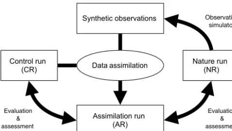
Figure 1.General flowchart of the BEATBOX system.
tensive collaboration between research entities. Approxima-tions are often required to make experiments possible (e.g., the “identical twin” problem), necessitating careful diagnosis of the results that could limit scientific conclusions.
Ultimately an OSSE should be used to highlight model deficiencies and inaccuracies, and provide direct guidance for model improvement. In that context, BEATBOX could be considered as a derived OSSE framework focused on data assimilation techniques and model improvement rather than the benefit of new or future types of observations. Starting from a scientific question or hypothesis to be validated (or rejected) that fits the topics mentioned above, several com-ponents are required (Fig. 1):
– a nature run (NR) considered as the “true state” (the NR supposes to use the best model representation possible considering the state of the art; in this study, we used the Master Chemical Mechanism (MCMv3.3.1) as the NR);
– a control run (CR) as the prior estimated state of the atmosphere (compared to the NR, a simplified or de-graded model should be used, for example a set of ODEs that can be implemented in large-scale 3-D mod-els; in this study, we use MOZART-T1);
– an observation simulator that generates synthetic obser-vation by sampling the NR (obserobser-vation errors also need to be simulated);
– an assimilation run (AR) that is produced using the data assimilation tool merging the synthetic observation with the CR to produce the best estimate possible of the state; and
– a suite of diagnostic tools that use NR, CR, and AR de-signed to point out model and data assimilation tech-nique limitations, ultimately providing a direct feedback for model improvement.
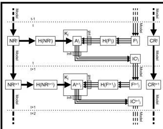
The BEATBOX framework has the capability to loop over several assimilation cycles, also called “cycling”. Cycling
with BEATBOX is schematically displayed in Fig. 2. Every cycle starts with the forecast step. By applying their respec-tive model, the NR, the forecast (F), and the CR are pro-cessed from cyclet−1 to cyclet. Then, NRtis used to
gen-erate synthetic observations through the observation opera-torH (see Sect. 2.2.2). These observations are assimilated into the forecast Ftj to produce the analysis Ajt withj as the data assimilation method of choice using a gainKj (see Sects. 2.2.3–2.2.5). Then,Ajt will be used to generate new initial conditions ICjt to start a new forecast. CRt serves as
a reference to determine the performance of the assimilation methodjaftertforecast cycles. The forecastFtjcan be taken to quantify the skill of the assimilation methodj at the cur-rent cyclet. Afterwards, the cyclet+1 starts with its forecast step.
2.1 Forecasting tool
2.1.1 The box model BOXMOX
BOXMOX performs box model simulations with different chemical mechanisms using varying sets of input parameters. BOXMOX relies on KPP, a code generator that simplifies the numerical integration of systems of ODEs. The tempo-ral evolution of concentrations of chemical compounds due to photochemistry is a prime example of such a system. KPP takes a predefined set of chemical equations (in our case a chemical mechanism) written in a symbolic, human-readable language and generates a computer code (FORTRAN, Mat-lab, C) containing a numerical solver to integrate the sys-tem over time. A number of integration methods are avail-able (e.g., Rosenbrock or Runge–Kutta methods). In addi-tion to predicting the evoluaddi-tion of concentraaddi-tions over time, the resulting solver also delivers the Jacobian and Hessian matrices of the system. Adjoint models can be generated and tuned (Sandu et al., 2003) and the Jacobians of the adjoint of the model can be obtained (see Sect. 2.2.3). Building upon KPP, BOXMOX provides additional processes typically used in box model studies (emissions, photolysis, deposition, mix-ing) and allows for convenient data input. BOXMOX makes simulations of chamber experiments, Lagrangian-type air parcel studies, and a description of the chemistry in the at-mospheric boundary layer feasible without effort. Input is done via simple text files: initial conditions, photolysis rates, temperature, boundary layer height, detrainment and entrain-ment, turbulent mixing, emission, and deposition are possi-ble input parameters. BOXMOX is a stand-alone C and For-tran program running on Linux or Mac OS X. In this work we have extended BOXMOX with an interface written in the Python language (boxmoxpackage) to interface more easily with BEATBOX.
chem-NRt
NRt+1
H(NRt)
H(NRt+1)
H(Ftj)
H(Ft+1j)
Ftj
Ft+1j
CRt
CRt+1
ICt+1j
Kj
Kj
Atj
At+1j
ICtj
Infl
Mo
de
l
Mo
de
l
Mo
de
l
Mo
de
l
Mo
de
l
Mo
de
l
Mo
de
l
Mo
de
l
Mo
de
l
Infl
Infl
Infl t-1
t
t t+1
t+1 t+2
Figure 2.The cycling sequence with BEATBOX, with the assimilation windowt, the assimilation methodj, control run CR, nature run NR, observation operatorH, gainK, analysisA, initial condition IC, and forecastF.
ical mechanism can be perturbed independently. Ensem-ble members can be generated by producing normal- or lognormal-distributed perturbation factors with the possibil-ity to adjust the mean and the standard deviation for each perturbed variable. These perturbation factors are then mul-tiplied by the relevant initial values to produce an ensemble of initial conditions.
In this work, we demonstrate the BEATBOX capabilities using MCMv3.3.1 as NR. Because of its near-explicit rep-resentation of atmospheric chemistry, MCMv3.3.1 is a good choice to be seen as the assumed “truth” within the context of an OSSE. The MOZART-T1 chemical mechanism is em-ployed as the simplified and/or degraded model (CR, AR). 2.1.2 Input data generation
BOXMOX comes with a tool to generate input data from field campaign observations (the genbox Python pack-age). Translation to mechanism-specific species naming and lumping is achieved using a translation tool (the
chemspectranslatorpackage) originally based on the
emission database created by Bill Carter (UC Riverside; http: //www.cert.ucr.edu/~carter/emitdb). The current system uses data collected in the FRAPPE (Front Range Air Pollution and Photochemistry Experiment) field campaign (frappedata
package).
During FRAPPE, a number of flight measurements with remote sensing and in situ devices of numerous
quanti-ties were performed, including concentrations of chemical species, photolysis rates, and temperature. In the examples shown we use measurements taken during FRAPPE with the NCAR C130 research aircraft to initialize the box model. Photolysis rates measured during FRAPPE are used in the examples shown here. For other cases in which photoly-sis rates are missing, we provide the ability to use photol-ysis rates calculated by the Tropospheric Ultraviolet Visible (TUV) radiation model version 5.1 (Madronich and Flocke, 1997) in BOXMOX using thetuvPython package.
In this current version of the code only measurements taken during the FRAPPE campaign have been used, but data from other field campaigns can be easily adapted as well with minimal code development.
2.2 Data assimilation tool
ThebeatboxtestbedPython package provides a data
2.2.1 The data assimilation problem
Data assimilation combines observations and model informa-tion (also called forecast or background) to derive an optimal state (analysis) with a reduced error to provide the best initial condition for a subsequent forecast (see, e.g., Lahoz et al., 2010). Considern∈Nandp∈Nthe dimensions of the state (or model) space and the observation space, respectively. Fol-lowing Nichols (2010) the solution to the data assimilation problem is commonly expressed as follows:
xa=xb+K(yo−H (xb)), (1)
wherexais the analysis state,xbthe background state,yothe
observation,Hthe observation operator (also known as for-ward operator in the variational formalism), andKthe gain matrix. The gain matrixKhandles the transformation from the observation space to the state (or model) space. Con-versely H handles the transformation from model space to observation space. The above equation can also be expressed in the incremental form, such as
1x=K1y, (2)
with1xcalled the increment and1ycalled the innovation (or departure). The innovation in the observation space is then translated to the model space by applying the gain ma-trixK. Different methods exist to estimate theKgain; see Sects. 2.2.3–2.2.5. Commonly the gain matrix is given by K=BHT HBHT+R−1
, (3)
where B and R are the error covariance matrices of the background (or model) and observation, respectively. In the BEATBOX framework a single observation in a given assim-ilation window (p=1) and only the dimension along the chemical variables is considered. Hence, R simplifies to a 1×1 matrix, a scalarσo2the observation error variance, and
HBHTalso simplifies to a scalarσb2(see Sect. 2.2.2 below) the background error variance in the observation space. Then BHTcan be seen asσb2s, wherescan be called the sensitiv-ity vector. The gain matrix in Eq. (3) then becomes a vector κ and can be reformulated as follows:
κ =σb2σb2+σo2
−1
s. (4)
2.2.2 Observation generator – synthetic observations Generating observations consists of the following steps:
– sampling values from the nature run,
– perturbing those values to simulate an observation inac-curacy, and
– specifying an observation error value.
BEATBOX forecasts have no dimensions in the 3-D at-mospheric space (latitude, longitude, altitude). Sampling the NR to simulate observations is straightforward. Convention-ally, H is defined as the observation operator and handles the transformation of information defined in the model space to the observation space to compare model and observa-tion quantities. Then, the H operator can be expressed as
HT= [0,0, . . .,1, . . .,0]. If no observation error is simulated the observation is defined as a perfect observation and the observation value isyo=H (xNR).
If the observation error needs to be simulated, thenyois
generated by adding a perturbation. In that version of BEAT-BOX the perturbation is assumed to be a normal distribution. But other probability density functions can be implemented easily (a lognormal perturbation is also implemented in this version). Then,
yo=H (xNR)+N (M, 6), (5)
withN (M, 6)as a normal distribution of meanMand stan-dard deviation6. The latter two quantities can be viewed as the observation bias or accuracy (M)and precision (6). Fi-nally, an associated observation errorσo is associated with yofor data assimilation;σocan account for bias and/or
pre-cision, overestimating, or underestimating those parameters depending on whether the effect of observation error needs to be tested in BEATBOX. In the following case study (see Sect. 3) we assume non-biased observation and non-biased observation error with a Gaussian distribution, leading to
σo=6.
2.2.3 Adjoint sensitivity
Adjoint sensitivities can be calculated using the KPP Jaco-bian matrix of output from the adjoint model at a given time step. In our case, we make the approximation that the change of the statex (that includes the observed variabley)at the time stept relative to the change of the observed variabley
at a previous time stept−1 (i.e., dxt/dyt−1or dyt/dyt−1)is
linear. In the current study, we assumet−1 andt at the be-ginning and the end of the assimilation window. The adjoint sensitivity vector of the statexto a given observed variable
y at timet can be computed using the Jacobian vectors as follows:
s=dxt dyt
= dxt dyt−1
·
dy
t
dyt−1
−1
. (6)
The adjoint assimilation method runs a single forecast with the forward model and also runs the adjoint model and com-putes the analysis by combining Eqs. (1), (4), and (6). The in-novation in observation space1yis calculated and the state xis inferred using theκ gain that includes the adjoint sensi-tivitys. In this method,σbshould be determined with ad hoc
between each cycle. In the BEATBOX context this can be further explored using the provided OSSE framework. 2.2.4 Ensemble sensitivity
Ensemble methods run a perturbed set (ensemble) of model realizations in parallel and derive model error and sensitivity using the created ensemble. This gives multiple realizations
i of the model in the observation spaceyi and model space
xi. The standard deviation of the ensemble (or the ensemble
spread) is used to estimateσbin the observation space, such
as σy=
r
Eh yi−Eyi 2i
=σb withEas the averaging
operator. Similarly, the ensemble spread in model space can be estimated as σx=
q
E(xi−E[xi])2
. Then statistical assumptions are made to derive the sensitivity betweenyand x. One of the commonly used methods as described by An-derson (2003) is to draw a linear fit in the least-squares sense betweenyandxusing the ensemble members, such as s=Xxiyi
X
yiyi
−1
=σxy
σ2 y
=rxy◦
σx
σy
, (7)
whererxyandσxyare respectively the correlation coefficient
and covariance vectors betweenyand each chemical variable ofxand◦is the Schur product operator. Then, the innovation in the observation space1yi is calculated for each ensemble
member. The ensemble state vector xi is inferred using the
samekgain that includes the same ensemble sensitivitysfor each ensemble member.
2.2.5 Hybrid sensitivity and further approaches In the current version of BEATBOX the hybrid sensitivity is defined as a combination between the two approaches men-tioned above: it uses an adjoint sensitivity for each ensemble member, such as
si=
dxt,i
dyt,i
= dxt,i dyt−1,i
·
dy
t,i
dyt−1,i
−1
. (8)
In that sense, each ensemble member has its own adjoint sen-sitivity calculation si and its own innovation in observation
space1yi. This results in an independent or different
infer-ence on the state vector for each ensemble memberxi. This
method is just an example of what can be explored with the BEATBOX system. Because of the simplicity of the code and the low dimensionality of the problem, advanced techniques can be easily implemented and analyzed. Other hybrid meth-ods and filters, such as a polynomial filter or particle filters and their benefits for highly nonlinear systems, can be ex-plored with ease with the proposed framework as well. 2.2.6 Inflation
For ensemble methods, to avoid the filter divergence prob-lem (Fitzgerald, 1971), inflation algorithms are needed. In
the BEATBOX framework we included the inflation method as proposed by Anderson (2007), such as
xinfli = √
λ (xi−E[xi])+E[xi], (9)
withλcalled the covariance inflation factor that determines how much the ensemble membersxiare spread out from the
meanE[x]. Many different methods exist to estimateλ; it can be chosen as constant over time or adaptive given the ensemble spread in observation spaceσb, observation error σo, and the innovation norm from the ensemble mean θ=
|E[yi] −yo|. In the version of BEATBOX presented here we
calculateλas
λ=θ
2−σ2 o
σb2 . (10)
Ifλ is found to be smaller than 1, the ensemble spread is assumed to be large enough and no inflation is calculated. Straightforward computation ofλas above assumes linearity between observation space and model space, which is true in the current BEATBOX framework. More advanced ways to computeλas described in Anderson (2007, Appendix A) have been tested and implemented in BEATBOX and can be used as well. Finally, to conserve the positive definite nature of the ensembles and also prevent forcing ensemble members to zero that would otherwise be inflated to negative values, we reduce the inflation factor iteratively on every value of the state:
λ≤ E[xi]
xinfli −E[xi]
!2
. (11)
This is one of several methods to conserve the physical as-pects of the ensemble: it might under-disperse the ensemble in some cases of low concentrations but ensures that the in-flation is kept to physical values. In the BEATBOX frame-work, users can easily implement and explore new inflation methods for nonlinear, definite positive, and perturbation of highly sensitive systems, as in the case of reactive gas-phase chemistry.
2.2.7 Localization
One should consider to what extent the sensitivities should be relied on. Localization algorithms try to limit the im-pact on the analysis of errors in the sample covariance be-tween observations and model state variables (Mitchell and Houtekamer, 2000). Depending on the ensemble size or the mathematical assumptions to compute a sensitivity, a local-ization functionCshould be used to define where to apply the sensitivitys, such as
sloc=s◦C. (12)
In the current BEATBOX framework, it is possible to specify which species should be inferred, e.g., CT=
2.3 Flux method for model analysis
A flux tool has been included inboxmoxthat calculates the production and loss fluxes for a given chemical component. Consider the generalized chemical reactions, such as
X
i
[R]i−→k X
j
[P]j, (13)
withkcalled the rate constant. The chemical flux can be ex-pressed as
d[R]
dt = −
d[P]
dt = −k
Y
i
[R]i =k
Y
j
[P]j. (14)
For a given chemical component, a detailed budget of chem-ical production and loss can be made by identifying different chemical reactions. An example of the application of the flux tool is shown in Sect. 3.4.
3 Application to an urban pollution case study
In this section, we provide an example case study to show-case the capabilities of the BEATBOX framework.
3.1 Control run and nature run
Temperature, concentrations, and photolysis rates from the FRAPPE data (see Sect. 2.1.2) are used for initial condi-tions. In the present simulations, all environmental param-eters such as temperature and photolysis rates are kept con-stant. Interactions between the simulated box and the sur-rounding are neglected, and the box model simulation can be seen as “chemistry in a jar” similar to a chamber experiment without consideration of wall losses, in which only the tem-poral evolutions due to chemical reactions are allowed. Initial conditions for primary VOCs and inorganic compounds are provided using the FRAPPE observations.
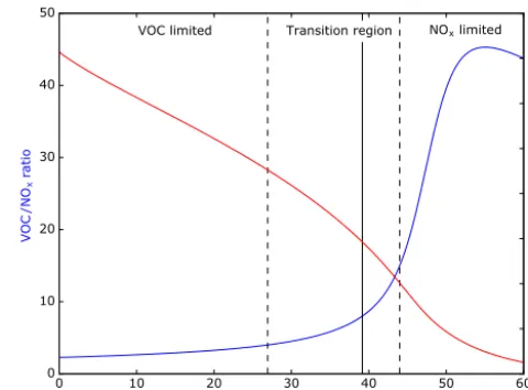
The present case study focuses on an air mass originat-ing from the industrial area of Commerce City near Den-ver, Colorado. Figure 3 shows the estimated temporal evo-lution over the first 60 h of simulation for the VOC/NOx
(NOx=NO+NO2) and toluene/benzene ratio using the
MOZART-T1 scheme. The vertical lines suggest the VOC-limited (VOC/NOxratio<=4), NOx-limited (VOC/NOx
ratio>15), and transition region (4<VOC/NOx
ra-tio<=15) to show that the simulation transitions through different O3 production regimes with possibly very
differ-ent relevant chemical pathways. The measuremdiffer-ents show an initially strongly VOC-limited air indicative of an urban air mass. The VOC/NOx ratio of the aging air increases in
time. During the first 15 h the simulation shows a strong VOC-limited regime. A transition regime spans from 15 h to approximately 30 h. After the transition period the chemi-cal regime becomes NOxlimited, which is representative of
0 10 20 30 40 50 60
Time in h 0
10 20 30 40 50
V
O
C
/N
Ox
r
a
ti
o
VOC limited Transition region NOx limited
0.0 0.5 1.0 1.5 2.0 2.5 3.0 3.5 4.0
T
o
lu
e
n
e
/b
e
n
ze
n
e
r
a
ti
o
Figure 3. Temporal evolution of the VOC/NOx (blue line) and toluene/benzene (red line) ratios over 60 h derived from MOZART-T1 (CR).
more rural or background conditions. The toluene/benzene ratio is used as a qualitative measure of photochemical age. Toluene and benzene are considered to have the same sources but toluene is more quickly oxidized than benzene, which leads to a decline in the ratio over time.
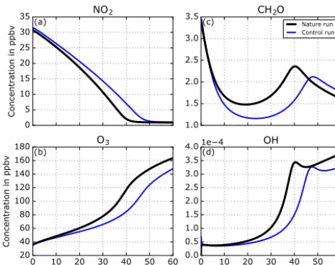
The temporal evolutions of some key species in the NR and the CR are displayed in Fig. 4. Nitrogen dioxide (NO2)
shows a decrease over time, with a stronger decay in the NR than in the CR. Ozone (O3)production is observed over time
with a therefore stronger production in the NR than in the CR. The hydroxyl-radical (OH) availability increases over time, especially between 20 and 35 h, which can be iden-tified as the end of the transition from a VOC-limited to a NOx-limited regime. In the VOC-limited and NOx-limited
regimes, the OH increase is smaller. Formaldehyde (CH2O)
shows in both NR and CR a decrease followed by an increase and finally a decrease. Those variations illustrate the change of chemical regimes from VOC limited to transition to NOx
limited. If we compare the NR to the CR the change of chem-ical regimes is lagged. The change of regimes seems to occur faster in the NR than in the CR, suggesting different reactiv-ity and pathways of oxidation in the NR than in the CR. 3.2 Assimilation runs
We focus on assimilating NO2 and CH2O concentrations
in two separate experiments to show the capabilities of the BEATBOX framework. This is motivated by the fact that NO2 and CH2O play a key role in atmospheric chemistry,
especially for short-lived chemical compounds. Also, NO2
and CH2O are, and will be, observed from space from both
low-Earth and geostationary orbiters and from in situ obser-vations. We define a reduced state vector for simplicity of the demonstration with the species described above: NO2, O3,
0 5 10 15 20 25 30 35
Concentration in ppbv
(a)
NO2
1.0 1.5 2.0 2.5 3.0 3.5
(c)
CH2O
Nature run Control run
0 10 20 30 40 50 60
Time in h 20
40 60 80 100 120 140 160 180
Concentration in ppbv
(b)
O3
0 10 20 30 40 50 60
Time in h 0.0
0.5 1.0 1.5 2.0 2.5 3.0 3.5
4.0 1e 4(d) OH
Figure 4.Time series of concentrations of NO2, O3, CH2O, and OH over 60 h from the control run (MOZART-T1, blue lines) and from the nature run (MCMv3.3.1, black lines).
We use an assimilation window of 3 h. Unbiased observa-tions have been defined and assumed to be at the end of the assimilation window with an observation error of 0.75 ppbv for NO2and 0.07 ppbv for CH2O (corresponding to
approx-imately 2.5 and 5 % of the concentrations at initial time). All the generated observations have well-estimated observation error, such as σo=6 (see Sect. 2.2.2). The model error in
the observation spaceσb has to be specified for the adjoint
technique and is set to 2.5 % for NO2and 5 % for CH2O of
the current forecast concentration (see Sect. 2.2.3). For the ensemble method, the ensemble spread implicitly definesσb
using 50 ensemble members that are generated by perturbing the initial NO2concentration by 2.5 % for NO2assimilation
and by perturbing the initial CH2O concentration by 5 % for
CH2O assimilation (see Sect. 2.2.4). Adaptive inflation is
ap-plied on the ensembles at every assimilation window to main-tain a realistic ensemble spread to weight the observation and model appropriately (see Sect. 2.2.6).
3.2.1 NO2assimilation
We assimilate NO2 observations using two different
local-izations. The first experiment infers only NO2concentration
and the second infers the entire state vector (i.e., NO2, O3,
CH2O, and OH concentrations). After looking at the
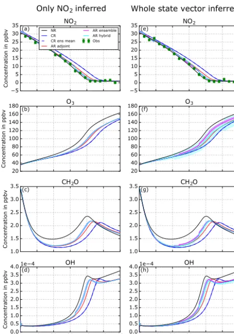
evolu-tion of NO2concentrations (see Fig. 5), all three assimilation
methods in both experiments (adjoint, ensemble, and hybrid) tend to move the analysis closer toward the observations and hence the NR. Some differences among the three ARs can be found. Recalling Sects. 2.2.1 and 2.2.2, because of the di-mensionality of the problem the sensitivity from observation space NO2 to the model variable NO2 is equal to identity,
s=1, for every assimilation method. Hence, the difference
among assimilation runs will only result from differences in xb and σb after a subsequent forecast. The ensemble and
hybrid methods show a quicker improvement than the sin-gle member adjoint method due to the adaptive nature ofσb
with the inflation (see Sect. 2.2.6). The single adjoint method keepsσb=2.5 %, while the ensemble and hybrid methods
can tune this value with the inflation.
When only NO2is inferred the other species are modified
and this could be called the model response to assimilated changes: NO2 is decreased, which increases the OH
avail-ability for other oxidation pathways. A slight increase in O3
is noted and more significantly for CH2O during the
transi-tion region. The ensemble methods have a stronger effect due to the adaptive nature ofσb. The adjustment of NO2
concen-tration towards NO2observation can be more effective and
this can have a stronger effect on the model response. When the entire state vector is inferred, i.e., no localiza-tion, slight additional increases occur in O3, CH2O, and OH
in the transition region. In general, in the first 10 to 15 h when VOC-limited conditions dominate (see Fig. 3), the impact of NO2 assimilation is low. By definition, VOC-limited air is
insensitive to changes in NO2, so if the model (CR) predicts
VOC-limited conditions either adjoint sensitivities or ensem-ble sensitivity will remain small. After 15 h of simulation, the chemical regime transitions significantly to NOx limited
with higher sensitivity of the state to changes in NO2.
Af-ter 40 h, NO2concentrations drop to very low values, NO2
assimilation increments are very small, and hence almost no inference on the other state variables is observed.
In the case study, inference from NO2observation on the
rest of vector is not the major reason for improvement. Model response from NO2 changes is mostly responsible for
im-proving the state. NOxconcentrations drive the chemistry in
the transition region and NOx-limited regimes. NOx
chem-istry is well known and similarly represented between the NR and the CR. Hence the model response is likely to improve the state and not likely to produce additional errors.
3.2.2 CH2O assimilation
We repeat the experiments presented in Sect. 3.2.1, but as-similate CH2O observations instead of NO2. Figure 6a–d
show the concentration evolution when only CH2O is
in-ferred. In the first 40 h CH2O is underestimated by the CR
mechanism. All three ARs show very similar results. During the analysis phases the CH2O concentrations are pushed up
towards the NR. Those abrupt increases are systematically compensated for by the chemical mechanism nudging the system back into chemical equilibrium, i.e., towards the CR concentrations. This makes the CH2O concentration
evolu-tion a sawtooth shape. CH2O is a short-lived chemical
com-pound (shorter than NO2in this case study) and it is mainly
driven by other chemical species concentrations. Ultimately CH2O concentrations in the ARs are slightly elevated after
5 0 5 10 15 20 25 30 35
Concentration in ppbv
(a)
NO2 NR CR CR ens mean AR adjoint AR ensemble AR hybrid Obs 5 0 5 10 15 20 25 30
35(e) NO2
20 40 60 80 100 120 140 160 180
Concentration in ppbv
(b) O3 20 40 60 80 100 120 140 160
180 (f) O3
1.0 1.5 2.0 2.5 3.0 3.5
Concentration in ppbv
(c)
CH2O
1.0 1.5 2.0 2.5 3.0
3.5(g) CH2O
0 10 20 30 40 50 60 Time in h
0.0 0.5 1.0 1.5 2.0 2.5 3.0 3.5 4.0
Concentration in ppbv
1e 4 (d)
OH
0 10 20 30 40 50 60 Time in h
0.0 0.5 1.0 1.5 2.0 2.5 3.0 3.5 4.0 1e 4(h)
Only NO2 inferred Whole state vector inferred
OH
Figure 5.Evolution of the state vector over 60 h, including the na-ture run (NR, black line), control run (CR, blue), and assimilation runs using adjoint (red), ensemble (pink), and hybrid (turquoise) methods. Two experiments with different localizations are dis-played: only NO2inferred(a–d)and whole state vector inferred(e– h). Shaded areas show corresponding ensemble spread for ensemble and hybrid methods.
state vector concentrations. The model response to CH2O
changes in NO2, O3, and OH is slight and definitely smaller
than the model response to NO2changes (see Sect. 3.2.1).
When the entire state vector is inferred, i.e., no localization (Fig. 6e–h), we observe very different results. The two ARs that are using adjoint sensitivities (hybrid and adjoint) show similar results as the previous experiment, and the sawtooth shape is still observed. The analysis shows strong increases in CH2O and the chemical mechanism tries to come back to
the CR state. The inference on the other species of the state vector is noticeable, and NO2, O3, and OH concentrations
are improved compared to the experiment when only NO2is
inferred.
In the ensemble method in which no localization is ap-plied, the improvement in CH2O is of a different nature.
The sawtooth behavior of the AR is not observed anymore and the chemical mechanism now seems to have changed
0 5 10 15 20 25 30 35
Concentration in ppbv
(a) NO2 0 5 10 15 20 25 30
35(e) NO2
20 40 60 80 100 120 140 160 180
Concentration in ppbv
(b) O3 20 40 60 80 100 120 140 160
180(f) O3
1.0 1.5 2.0 2.5 3.0 3.5 4.0
Concentration in ppbv
(c)
CH2O NR CR CR ens mean AR adjoint AR ensemble AR hybrid Obs 1.0 1.5 2.0 2.5 3.0 3.5
4.0(g) CH2O
0 10 20 30 40 50 60 Time in h
0.0 0.5 1.0 1.5 2.0 2.5 3.0 3.5 4.0
Concentration in ppbv
1e 4 (d)
OH
0 10 20 30 40 50 60 Time in h
0.0 0.5 1.0 1.5 2.0 2.5 3.0 3.5 4.0 1e 4(h)
Only CH2O inferred Whole state vector inferred
OH
Figure 6.Same as Fig. 5 but with CH2O observations assimilated.
from systematic CH2O loss to CH2O production in the
fore-cast. This will drive the AR to better fit the observations and hence the NR. The inference on other species shows signifi-cant changes that will in general change the sign of the error and sometimes increase it; NO2becomes underestimated in
the transition region, O3 is overestimated but then
underes-timated after 35 h, and OH is overesunderes-timated in the transition region. In the ensemble method for the case study, the com-puted sensitivities seem significantly different from the ad-joint sensitivities. This will allow us to change the chemical production and loss rate of CH2O to better adjust the CH2O
concentration, but at the risk of disturbing the rest of the state vector and increasing errors that might lead to unphysical re-sults. We diagnose the difference among sensitivities from the two experiments presented above in Sect. 3.3. We also diagnose the chemical behavior change from CH2O
assimi-lation using fluxes in Sect. 3.4.
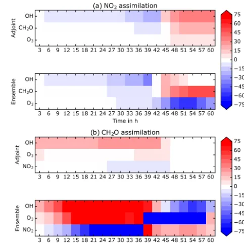
3.3 Sensitivities of the off-diagonal elements of the background error covariance matrix
assimilation window with the single member adjoint and the ensemble method (see Sects. 2.2.3 and 2.2.4). To make sen-sitivities comparable we have normalized (divided) them by the state concentrations. For example,s(NO2,O3), the
sensi-tivity of NO2changes over O3, will most likely be orders of
magnitude larger thans(NO2,OH)since O3concentrations
are orders of magnitude larger than OH concentrations. For NO2 assimilation, both methods deliver similar
re-sults. The sensitivities are in general small, not above 60 %. Sensitivities are small or negligible in the VOC-limited regime but become more significant during the transition and the NOx-limited regimes, mostly after 30 h. The changes in
NO2from assimilation after 30 h are rather small and hence
the inference on other species will be small. This then con-firms that the most important part of the changes from NO2
assimilation is due to the model response from NO2changes
and secondly due to the data assimilation inference on the other species of the state.
For CH2O assimilation we saw significant differences in
behavior between adjoint and ensemble methods to compute the sensitivities. The adjoint displays rather small sensitivi-ties, peaking at 20 % but mostly below 10 %. Those sensitives are observed during the VOC-limited regime when the chem-istry is sensitive to changes from VOC concentrations and disappear during the transition region and become insignifi-cant in the NOx-limited regime. This explains the small but
reasonable impacts from CH2O changes on the rest of the
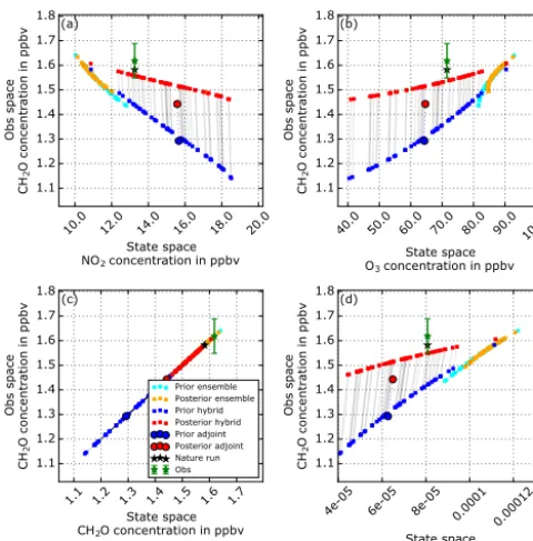
state. Concerning the ensemble method, the computed sensi-tivities are much larger and do not decrease after the transi-tion regime. Values switch abruptly from negative to positive and are sometimes above 200 %. To understand this unphys-ical behavior, we display tracer–tracer relationships during the assimilation phase of the ninth cycle (27 h) in Fig. 8.
In Sect. 2.2.4, we defined the ensemble method sensitiv-ity computation as a linear fit to the ensemble distribution between two species. Most state-of-the-art EnKF methods use this approximation. One can see the limitation to such a linear assumption after looking carefully at Fig. 8a and b. The prior and posterior states of the NO2–O3distributions
are displayed. The ensemble method represents the observa-tion well; the ensemble distribuobserva-tion is at the NO2level of the
observation and the ensemble spread fits the observation er-ror (green vertical bars). However, the relationship between NO2and O3that has formed during the ensemble AR after
nine cycles is strongly curved and nonlinear, which is diffi-cult to represent through the linear fit of the ensemble sensi-tivity. In this example, moving the ensemble members along the linear fit is moving the O3distribution slightly away from
the NR. At the same time the adjoint sensitivities are in com-parison very weak (the slope is along theyaxis), slightly im-proving the state distributions but not very strongly. Finally, the hybrid distribution shows a larger spread and different distribution shape than the ensemble distribution. The ad-joint inference does not strongly change the rest of the state, which maintains the chemical production and loss rates of
3 6 9 12 15 18 21 24 27 30 33 36 39 42 45 48 51 54 57 60 O3
CH2O OH
Adjoint
(a) NO2 assimilation
3 6 9 12 15 18 21 24 27 30 33 36 39 42 45 48 51 54 57 60 Time in h
O3 CH2O OH
Ensemble 75
60 45 30 15 0 15 30 45 60 75
S
en
si
ti
vi
ty
t
o
1
p
p
b
v
N
O2
c
h
an
g
e
to the state in %
3 6 9 12 15 18 21 24 27 30 33 36 39 42 45 48 51 54 57 60 NO2
O3 OH
Adjoint
(b) CH2O assimilation
3 6 9 12 15 18 21 24 27 30 33 36 39 42 45 48 51 54 57 60 Time in h
NO2 O3 OH
Ensemble 75
60 45 30 15 0 15 30 45 60 75
S
en
si
ti
vi
ty
t
o
1
p
p
b
v
C
H2
O
c
h
an
g
e
to the state in %
Figure 7.Temporal evolution of the sensitivities of the unobserved state species to changes from the observed one at the end of each 3 h assimilation for NO2assimilation(a)and CH2O assimilation(b).
CH2O that fall into a temporary attractor; the model wants
to go back to the CR concentrations and creates a sawtooth-shaped concentration evolution over time (see Sect. 3.2.2). After 3 h, the forecast will be significantly far from the ob-servation and the distribution will be inflated. The ensemble inference strongly changes the rest of the state, which will change the chemical production and loss rates and drive the system out of the attractor. To understand this more clearly, the flux tool is presented in the following section.
3.4 Model diagnostics using fluxes
In this last section, we will focus on the CH2O fluxes
(pro-duction and loss) over the ninth cycle forecast (25 to 27 h) of the CH2O assimilation without localization. In Fig. 9
are the individual contributions of production and loss of CH2O for the NR and the same member of the CR, AR
en-semble, and AR hybrid. The flux tool isolates a few differ-ent reactions with NR because the chemical scheme is dif-ferent and more detailed than the CR. In this case study, CH3O→CH2O+HO2 in the NR is simply an
intermedi-ate reaction of NO+CH3O2→CH2O+NO2+HO2. Other
than this reaction, the isolated reactions are similar.
10.0 12.0 14.0 16.0 18.0 20.0
State space NO2 concentration in ppbv 1.1 1.2 1.3 1.4 1.5 1.6 1.7 1.8 Obs space C H2 O c o n ce n tr a ti o n in p p b v (a)
40.0 50.0 60.0 70.0 80.0 90.0 100.0
State space O3 concentration in ppbv 1.1 1.2 1.3 1.4 1.5 1.6 1.7 1.8 Obs space C H2 O c o n ce n tr a ti o n in p p b v (b)
1.1 1.2 1.3 1.4 1.5 1.6 1.7
State space CH2O concentration in ppbv 1.1 1.2 1.3 1.4 1.5 1.6 1.7 1.8 Obs space C H2 O c o n ce n tr a ti o n in p p b v (c) Prior ensemble Posterior ensemble Prior hybrid Posterior hybrid Prior adjoint Posterior adjoint Nature run Obs
4e-05 6e-05 8e-05 0.0001 0.00012
State space OH concentration in ppbv 1.1 1.2 1.3 1.4 1.5 1.6 1.7 1.8 Obs space C H2 O c o n ce n tr a ti o n in p p b v (d)
Figure 8.Tracer–tracer or observation space to state space relation-ships during the ninth cycle of the CH2O assimilation without lo-calization experiment.
concentration evolution) also differ. The production terms are stronger, leading to almost no loss net flux. The order of importance of the reactions in the budget is also different; CH2O+OH→CO+HO2+H2O is much more important,
likely due to the increase in OH during the AR ensemble (see Sect. 3.2.2). Finally, the AR hybrid fluxes are similar to the CR fluxes with the same order of importance between reac-tions. Except for the carbon monoxide (CO) formation from photolysis, CH2O→CO+H2is now stronger and is
respon-sible for the systematic decrease in CH2O in the AR adjoint
and AR hybrid (see Sect. 3.2.2). This increased flux from this reaction explains the sawtooth behavior of CH2O. When no
other pathway of loss is possible, i.e., OH is not as strongly changed in AR adjoint and hybrid as in AR ensemble, this way of destroying CH2O is then increased.
We demonstrate here the usefulness of the flux tool to di-agnose the effect of data assimilation on atmospheric chem-istry in a detailed manner. The diagnostic of the flux tool can be used on any species that a chemical scheme contains for any kind of BOXMOX simulation.
4 Summary and future options
In this paper, we have presented a new suite of tools for box models, BEATBOX. The design of BEATBOX is based on an OSSE approach that can simultaneously integrate vari-ous chemical schemes to simulate a nature run, control runs, and assimilation runs. This framework includes the
capabil-0.4 0.2 0.0 0.2 0.4 0.6 Fl u x in p p b v h − 1 (a)
NR (MCM v3.3)
CH2O + OH -> CO + HO2
CH3O -> CH2O + HO2
CH2O -> CO + 2 HO2
CH3OH + OH -> CH2O + HO2
CH2O -> H2 + CO
0.4 0.2 0.0 0.2 0.4 0.6 (b) EN (MOZART-4)
CH3OH + OH -> CH2O + HO2
CH2O + OH -> CO + HO2 + H2O CH2O -> CO + 2 HO2
CH2O -> H2 + CO
NO + CH3O2 -> CH2O + NO2 + HO2
0.4 0.2 0.0 0.2 0.4 0.6 Fl u x in p p b v h − 1 (c) AR_ens (MOZART-4)
CH3OH + OH -> CH2O + HO2
CH2O + OH -> CO + HO2 + H2O
CH2O -> CO + 2 HO2
CH2O -> H2 + CO
NO + CH3O2 -> CH2O + NO2 + HO2
0.0 0.5 1.0 1.5 2.0 2.5 3.0 Time in h
0.4 0.2 0.0 0.2 0.4 0.6 (d) AR_hyb (MOZART-4)
CH3OH + OH -> CH2O + HO2
CH2O + OH -> CO + HO2 + H2O
CH2O -> CO + 2 HO2
CH2O -> H2 + CO
NO + CH3O2 -> CH2O + NO2 + HO2
0.0 0.5 1.0 1.5 2.0 2.5 3.0 Time in h
0.20 0.15 0.10 0.05 0.00 0.05 0.10 Fl u x in p p b v h − 1 (e) Net fluxes NR EN AR_ens AR_hyb
Figure 9.CH2O fluxes during the 3 h forecast of the ninth cycle of the CH2O assimilation with no localization. For the NR(a), one member of the CR(b), one member of the AR ensemble(c), and one member of the AR hybrid(d). Net fluxes for each run are shown in panel(e). Displayed are fluxes representative of 90 % of the budget.
ity of running assimilation windows of different chemical schemes using a forecasting tool (BOXMOX) and an assimi-lation tool allowing for sensitivity analysis. BEATBOX pro-vides ensemble and adjoint sensitivity analyses that can be combined or modified to explore new inverse or data assim-ilation methodologies. Additionally, a flux tool is also inte-grated into the framework to diagnose and assess in detail model run differences and ultimately use data assimilation to improve the model (chemical scheme) itself, not only the model outputs. The systematic and detailed assessment of the multivariate data assimilation problem indicates that BEAT-BOX can tackle important scientific hypotheses at a limited computational cost for future data assimilation configura-tions in large-scale 3-D models for atmospheric chemistry, but it is not limited to this. Any system of equations can be integrated over time in the current framework.
A typical case study of ozone photochemical production from NOx is presented to showcase the capability of
BEAT-BOX. Differences between the nature run and the control run are presented followed by a data assimilation experiment of synthetic NO2and CH2O observations using adjoint and
to understand in detail the effect of data assimilation in a complicated and nonlinear model as required by atmospheric chemistry. In these case studies, we showcased BEATBOX as a powerful and user-friendly tool for the following:
– understanding chemical mechanism differences and de-ficiencies,
– performing chemical sensitivity analysis using ensem-ble or adjoint methods,
– envisioning and designing new inverse and data assim-ilation methods for atmospheric chemistry to optimally constrain as much of the chemical state as possible, – defining requirements for new chemical and data
assim-ilation schemes and ultimately improving them, and – educational purposes for data assimilation and
atmo-spheric chemistry.
BEATBOX will continue to evolve according to user re-quirements. For example, emission inversion capability is currently being implemented. Setting any given observation time into the assimilation window will also be possible. As-similating multiple observations in a given assimilation win-dow will also be implemented using sequential and varia-tional minimization techniques. Using real observations, i.e., from field campaigns, is also possible with minimal code modifications. Because of the user friendliness, flexibility, and open source nature of most of BOXMOX–BEATBOX, users could also contribute to model development and make it a broad atmospheric chemistry community tool.
Code and data availability. All code developments presented here are open source tools released under the GNU General Public Li-cense v3. BEATBOX consists of a number of Python packages:
– beatboxtestbed(the BEATBOX Background Error Anal-ysis Testbed),
– boxmox(Python interface for the chemical box model BOX-MOX),
– genbox(input data generator forboxmox),
– frappedata(FRAPPE campaign dataset forgenbox), – tuv(TUV data connector forgenbox),
– chemspectranslator(translator to translate species be-tween chemical mechanisms and observations), and
– icartt(reader–writer for ICARTT files).
The underlying chemical box model BOXMOX is a stand-alone C and Fortran executable and has to be installed before BEATBOX can be used.
Source code version 1.0 used in this paper is archived online at digital object identifier: 10.5281/zenodo.1118244 (Knote et al., 2017). Full documentation for BOXMOX and all Python packages, including examples on how to reproduce the case studies shown in this paper, can be found at https://boxmodeling.meteo.physik. uni-muenchen.de/documentation.
Author contributions. CK and JB contributed equally to the paper. CK designed the BOXMOX system, wrote the framework around BEATBOX, supervised ME, and contributed to writing the paper. JB came up with the idea for BEATBOX and coded most of the beatbox.py routine, co-supervised ME, and wrote most of the paper. ME developed parts of the BEATBOX framework during his Mas-ters thesis, prepared and analyzed the case studies, and contributed the flux tool.
Competing interests. The authors declare that they have no conflict of interest.
Acknowledgements. We thank the many scientists who contributed to the FRAPPE field campaign for providing useful data to initialize the model simulations. Frank Flocke and Rebecca Hornbrook (NCAR) are thanked for creating the Commerce City sample used in the case studies. We acknowledge Bill Carter (UC Riverside) for his work on the emission database. We ac-knowledge support from NASA KORUS-AQ grant NNX16AD96G.
Edited by: Tim Butler
Reviewed by: two anonymous referees
References
Anderson, J. L.: A local least squares framework for ensemble fil-tering, Mon. Weather Rev., 131, 634–642, 2003.
Anderson, J. L.: An adaptive covariance inflation error correction algorithm for ensemble filters, Tellus A, 59, 210–224, 2007. Archibald, A. T., Jenkin, M. E., and Shallcross, D. E.: An isoprene
mechanism intercomparison, Atmos. Environ., 44, 5356–5364, https://doi.org/10.1016/j.atmosenv.2009.09.016, 2010.
Arnold, C. P. and Dey, C. H.: Observing-systems simulation exper-iments: Past, present, and future, B. Amer. Meteorol. Soc., 67, 687–695, 1986.
Barré, J., Edwards, D., Worden, H., Silva, A. D., and Lahoz, W.: On the feasibility of monitoring carbon monoxide in the lower tropo-sphere from a constellation of northern hemitropo-sphere geostationary satellites (part 1). Atmos. Environ., 113, 63–77, 2015.
Barré, J., Edwards, D., Worden, H., Arellano, A., Gaubert, B., Silva, A. D., Lahoz, W., and Anderson, J.: On the feasibility of moni-toring carbon monoxide in the lower troposphere from a con-stellation of northern hemisphere geostationary satellites: Global scale assimilation experiments (part II), Atmos. Environ., 140, 188–201, 2016.
Claeyman, M., Attié, J.-L., Peuch, V.-H., El Amraoui, L., La-hoz, W. A., Josse, B., Joly, M., Barré, J., Ricaud, P., Massart, S., Piacentini, A., von Clarmann, T., Höpfner, M., Orphal, J., Flaud, J.-M., and Edwards, D. P.: A thermal infrared instru-ment onboard a geostationary platform for CO and O3 measure-ments in the lowermost troposphere: Observing System Simula-tion Experiments (OSSE), Atmos. Meas. Tech., 4, 1637–1661, https://doi.org/10.5194/amt-4-1637-2011, 2011.
At-mos. Chem. Phys., 15, 8795-8808, https://doi.org/10.5194/acp-15-8795-2015, 2015.
Edwards, D. P., Arellano Jr., A. F., and Deeter, M. N.: A satellite observation system simulation experiment for carbon monoxide in the lowermost troposphere, J. Geophys. Res., 114, D14304, https://doi.org/10.1029/2008JD011375, 2009.
Emmerson, K. M. and Evans, M. J.: Comparison of tropospheric gas-phase chemistry schemes for use within global models, At-mos. Chem. Phys., 9, 1831–1845, https://doi.org/10.5194/acp-9-1831-2009, 2009.
Emmons, L. K., Walters, S., Hess, P. G., Lamarque, J.-F., Pfis-ter, G. G., Fillmore, D., Granier, C., Guenther, A., Kinnison, D., Laepple, T., Orlando, J., Tie, X., Tyndall, G., Wiedinmyer, C., Baughcum, S. L., and Kloster, S.: Description and eval-uation of the Model for Ozone and Related chemical Trac-ers, version 4 (MOZART-4), Geosci. Model Dev., 3, 43–67, https://doi.org/10.5194/gmd-3-43-2010, 2010.
Fitzgerald, R.: Divergence of the Kalman filter, IEEE T. Automat. Contr., 16, 736–747, 1971.
Jenkin, M. E., Young, J. C., and Rickard, A. R.: The MCM v3.3.1 degradation scheme for isoprene, Atmos. Chem. Phys., 15, 11433–11459, https://doi.org/10.5194/acp-15-11433-2015, 2015.
Knote, C., Hodzic, A., Jimenez, J. L., Volkamer, R., Orlando, J. J., Baidar, S., Brioude, J., Fast, J., Gentner, D. R., Goldstein, A. H., Hayes, P. L., Knighton, W. B., Oetjen, H., Setyan, A., Stark, H., Thalman, R., Tyndall, G., Washenfelder, R., Waxman, E., and Zhang, Q.: Simulation of semi-explicit mechanisms of SOA formation from glyoxal in aerosol in a 3-D model, At-mos. Chem. Phys., 14, 6213–6239, https://doi.org/10.5194/acp-14-6213-2014, 2014.
Knote, C., Tuccella, P., Curci, G., Emmons, L., Orlando, J. J., Madronich, S., Barò, R., Jimènez-Guerrero, P., Luecken, D., Hogrefe, C., Forkel, R., Werhahn, J., Hirtl, M., Pèrez, J. L., San Josè, R., Giordano, L., Brunner, D., Yahya, K., and Zhang, Y.: Influence of the choice of gas-phase mechanism on predictions of key gaseous pollutants during the AQMEII phase-2 intercom-parison, Atmos. Environ., 115, 553–568, 2015.
Knote, C., Barré, J., and Eckl, M.: BEATBOX v1.0: Background Er-ror Analysis Testbed with Box Models (Version 1.0.0), Zenodo, https://doi.org/10.5281/zenodo.1118244, 19 December 2017. Kuo, Y.-H., Zou, X., and Huang, W.: The impact of global
po-sitioning system data on the prediction of an extratropical cy-clone: an observing system simulation experiment, Dynam. At-mos. Oceans, 27, 439–470, 1998.
Lahoz, W., Khattatov, B., and Mènard, R. (Eds.): Data Assimila-tion: Making Sense of Observations, Springer Berlin Heidelberg, 718 pp., 2010.
Liu, C., Xiao, Q., and Wang, B.: An ensemble-based four-dimensional variational data assimilation scheme, part II: Ob-serving system simulation experiments with advanced research WRF (ARW), Mon. Weather Rev., 137, 1687–1704, 2009. Madronich, S. and Flocke, S.: Theoretical Estimation of
Biologi-cally Effective UV Radiation at the Earth’s Surface, Springer, Berlin Heidelberg, 23–48, 1997.
Mazzuca, G. M., Ren, X., Loughner, C. P., Estes, M., Craw-ford, J. H., Pickering, K. E., Weinheimer, A. J., and Dick-erson, R. R.: Ozone production and its sensitivity to NOx and VOCs: results from the DISCOVER-AQ field experi-ment, Houston 2013, Atmos. Chem. Phys., 16, 14463–14474, https://doi.org/10.5194/acp-16-14463-2016, 2016.
Mitchell, H. L. and Houtekamer, P. L.: An adaptive ensemble Kalman filter, Mon. Weather Rev., 128, 416–433, 2000. Nichols, N. K.: Mathematical Concepts of Data Assimilation, in:
Data assimilation: making sense of observations, edited by: La-hoz, W., Khattatov, B. and Menard, R., Springer, 13–39, 2010. Ott, E., Hunt, B., Szunyogh, I., Zimin, A., Kostelich, E., Corrazza,
M., Kalnay, E., and Yorke, J.: A local ensemble Kalman filter for atmospheric data assimilation, Tellus A, 56, 415–428, 2004. Sandu, A. and Sander, R.: Technical note: Simulating
chem-ical systems in Fortran90 and Matlab with the Kinetic PreProcessor KPP-2.1, Atmos. Chem. Phys., 6, 187–195, https://doi.org/10.5194/acp-6-187-2006, 2006.
Sandu, A., Daescu D., and Carmichael G. R.: Direct and adjoint sensitivity analysis of chemical kinetic systems with KPP: Part I – theory and software tools, Atmos. Environ., 37, 5083–5096, https://doi.org/10.1016/j.atmosenv.2003.08.019, 2003.
Sandu, A., Daescu, D. N., Carmichael, G. R., and Chai, T.: Ad-joint sensitivity analysis of regional air quality models, J. Com-put. Phys., 204, 222–252, 2005.
van Leeuwen, P. J.: Nonlinear data assimilation in geosciences: an extremely efficient particle filter, Q. J. Roy. Meteor. Soc., 136, 1991–1999, https://doi.org/10.1002/qj.699, 2010.
Wang, X., Barker, D. M., Snyder, C., and Hamill, T. M.: A hybrid ETKF-3DVar data assimilation scheme for the WRF model, Part I: Observing system simulation experiment, Mon. Weather Rev., 136, 5116–5131, 2008.