www.geosci-model-dev.net/4/1103/2011/ doi:10.5194/gmd-4-1103-2011
© Author(s) 2011. CC Attribution 3.0 License.
Geoscientific
Model Development
Evaluation of a Global Vegetation Model using time series of
satellite vegetation indices
F. Maignan1, F.-M. Br´eon1, F. Chevallier1, N. Viovy1, P. Ciais1, C. Garrec1, J. Trules1, and M. Mancip2 1Laboratoire des Sciences du Climat et de l’Environnement, IPSL, UMR8212 (CEA/CNRS/UVSQ), CEA Saclay,
Orme des Merisiers, 91191 Gif sur Yvette CEDEX, France
2Institut Pierre Simon Laplace, Universit´e Pierre et Marie Curie, 4 place Jussieu, 75252 Paris CEDEX 05, France
Received: 27 March 2011 – Published in Geosci. Model Dev. Discuss.: 29 April 2011 Revised: 17 November 2011 – Accepted: 19 November 2011 – Published: 5 December 2011
Abstract. Atmospheric CO2drives most of the greenhouse
effect increase. One major uncertainty on the future rate of increase of CO2in the atmosphere is the impact of the
an-ticipated climate change on the vegetation. Dynamic Global Vegetation Models (DGVM) are used to address this ques-tion. ORCHIDEE is such a DGVM that has proven useful for climate change studies. However, there is no objective and methodological way to accurately assess each new avail-able version on the global scale. In this paper, we submit a methodological evaluation of ORCHIDEE by correlating satellite-derived Vegetation Index time series against those of the modeled Fraction of absorbed Photosynthetically Active Radiation (FPAR). A perfect correlation between the two is not expected, however an improvement of the model should lead to an increase of the overall performance.
We detail two case studies in which model improvements are demonstrated, using our methodology. In the first one, a new phenology version in ORCHIDEE is shown to bring a significant impact on the simulated annual cycles, in par-ticular for C3 Grasses and C3 Crops. In the second case study, we compare the simulations when using two differ-ent weather fields to drive ORCHIDEE. The ERA-Interim forcing leads to a better description of the FPAR interannual anomalies than the simulation forced by a mixed CRU-NCEP dataset. This work shows that long time series of satellite observations, despite their uncertainties, can identify weak-nesses in global vegetation models, a necessary first step to improving them.
Correspondence to: F. Maignan
(maignan@lsce.ipsl.fr)
1 Introduction
Dynamic Global Vegetation Models (DGVM) quantify en-ergy and mass fluxes between the surface and the atmo-sphere. They are either used as a component within mete-orological forecasting schemes and climate models or they are used in a stand-alone mode, forced by weather and cli-mate fields, to help to quantify and understand the variability of carbon, water or nutrients fluxes and pools. One major uncertainty for the future rate of increase of CO2in the
at-mosphere is the impact of the anticipated climate change on the vegetation (IPCC, 2007). An increase of CO2is expected
to have beneficiary impacts on the vegetation photosynthe-sis and growth (leading to a net sink of carbon). However, changes in temperature, radiation and precipitation, as a re-sult of CO2 induced climate change, can have either
focus here on the global scale, using satellite measurements to evaluate model outputs. Even if a model modification is evaluated favorably when comparing model outputs with measurements at sites, it still has to be evaluated with ded-icated global tools, such as the one we present here, when applied on a global scale.
The objectives of this paper are twofold. First, we present a robust method for a quantitative evaluation of any DGVM performance using properly calibrated and corrected satel-lite time series. Second, we apply this method to evaluate the performances of different versions of the ORCHIDEE vegetation model (different phenologies and different climate drivers).
The model and satellite data are described in Sect. 2. Sec-tion 3 details the methodology and Sects. 4 and 5 present the results. Discussion and conclusions are given in Sect. 6.
2 Model and data
2.1 The ORCHIDEE model
ORCHIDEE (Krinner et al., 2005) is a DGVM developed at the Institut Pierre Simon Laplace (IPSL). It models carbon, water and energy fluxes as well as the dynamics of biomass, soil carbon and soil water pools. It has been used at the site level (Jung et al., 2007a) and on a global scale (Krinner et al., 2005; Piao et al., 2008). The current version (1.9.5) is available on request to the authors.
ORCHIDEE models the dynamics of 13 different Plant Functional Types (PFT) (Prentice et al., 1992). Each PFT contains different plant species which grow under similar soil properties and climatic factors (temperature and precipita-tion), and which share the same physiological processes such as cold tolerance, or water needs (Cramer, 2002). The dy-namics of each PFT are controlled by a common set of equa-tions but with different parameters. An exception is the phe-nology, for which each PFT is assigned a specific set of equa-tions as described in Botta et al. (2000). The ORCHIDEE model can either use a fixed distribution of PFTs (with frac-tional coverage specified for each model grid) or it can cal-culate the PFT distribution dynamically, according to local climate and competition between different PFTs. As we are evaluating the model over a short recent period, we chose to use a fixed vegetation distribution, derived from recent ob-servations, rather than a dynamic one. The state of the art models of vegetation dynamics are still rather crude and lead to biases in simulated vegetation types as compared to the ob-servations (Krinner et al., 2005; Bonan and Levis, 2006). Ta-ble 1 shows the list of the 13 PFTs along with their acronym used in this paper.
The various versions of the ORCHIDEE model are due ei-ther to structural changes (i.e. changes in the processes or the controlling parameters) or to different input parameters, such as meteorological forcing fields. An objective methodology
Table 1. Vegetation types and their abbreviations as used in ORCHIDEE.
PFT Name Abbreviation
1 Bare soil Bare
2 Tropical Broad-leaved Evergreen TroBroEver 3 Tropical Broad-leaved Raingreen TroBroRain 4 Temperate Needleleaf Evergreen TempNeedleEver 5 Temperate Broad-leaved Evergreen TempBroEver 6 Temperate Broad-leaved Summer-green TempBroSum 7 Boreal Needleleaf Evergreen BorNeedleEver 8 Boreal Broad-leaved Summer-green BorBroSum 9 Boreal Needleleaf Summer-green BorNeedleSum
10 C3 Grass C3grass
11 C4 Grass C4grass
12 C3 Crops C3crops
13 C4 Crops C4crops
is needed for the evaluation of these versions, in order to further improve carbon fluxes estimates on a global scale. The primary carbon flux calculated by ORCHIDEE is the Gross Primary Productivity (GPP). In a study by Jung et al. (2007b), it was shown that the modeling of GPP was pri-marily sensitive to differences between models rather than to differences in meteorological forcing. We assume that these conclusions should also hold for the Leaf Area Index (LAI), as it is closely related to the GPP. We will therefore focus on this ORCHIDEE key-variable as it can be compared to actual satellite data. In this paper, we will thus evaluate the impact of structural changes in the phenology model on the modeled LAI, and the impact of two different global meteorological forcing fields.
2.1.1 The phenology models
ORCHIDEE implements a prognostic leaf cycle through cli-mate driven leaf onset models, and leaf senescence processes governing turnover rates.
The climate driven leaf onset phenological models in ORCHIDEE are mainly derived from the work of Botta et al. (2000). The authors used AVHRR satellite data to select and calibrate local phenology models (Chuine, 2000) for the global scale, for approximately ten biomes. In ORCHIDEE, the Summer-green PFTs leaf onset is driven by air tem-perature only. The two Broad-leaved Summer-green PFTs use a classical Growing-Degree-Day (GDD) model, where the GDD cut-off value depends on the Number of Chill-ing Days (NCD), followChill-ing a decreasChill-ing exponential rela-tionship. The Boreal Needleleaf Sumer-green PFT (mainly
Larix decidua) model uses a simple Number of Growing
The leaf senescence is driven by two different processes: the first one depends on climatic conditions and the sec-ond one depends on a critical leaf life span. In the climate driven senescence models, the process for all Summer-green PFTs is based on conditions related to temperature decrease and the one for the Tropical Broad-leaved Raingreen PFT is based on a lesser moisture availability condition. For all Tree PFTs, when senescence is declared a predefined turnover rate is set. The senescence model for the Grass and Crop PFTs is a mixed one, with temperature and moisture availability conditions governing a climate dependent turnover rate. In the leaf age related senescence models, a mean leaf life span is set for each PFT, and the turnover rate of leaves increases sharply where mean leaf age reaches the leaf life span. Leaf senescence of Evergreen PFTs is only driven by leaf age.
In the current version, two drawbacks have been identified by users and the new phenology scheme is based on the cor-rections proposed below for these drawbacks. The first draw-back is related to the choice of the reference date at which the GDD calculation begins. This date is variable and cor-responds to the end of the former growing cycle. Although functionally realistic, this system generates chaotic behavior (due to non-linear onset and senescence phenological mod-els using thresholds) and leads, for Grasses and Crops, to a seemingly erratic tendency of “grow and decay”. This results in very irregular LAI time series, with unrealistically large interannual variations compared to the observations. On the other hand, a fixed date cannot be chosen as ORCHIDEE is designed to run for a wide range of time periods and cli-mates, including paleo-climates. For these reasons, the new phenology scheme uses the winter solstice, calculated for each orbital condition, as the reference date for GDD cal-culations. Fixing the date for the start of GDD calculations for any given simulation leads to a more stable phenological cycle.
The second drawback in the current ORCHIDEE version is that crops share the same leaf onset and senescence cli-mate driven phenology models as grasses. This is quite un-realistic, even with different PFT parameters, as the crop growing season length is generally much shorter than that of grasses because the harvest abruptly terminates the sea-sonal cycle. A complex approach for crop representation was developed by coupling ORCHIDEE to the STICS agro-nomic model (Gervois et al., 2008), but this option is not yet included in the current ORCHIDEE version. In parallel, a simpler approach has been adopted in the new phenology version, which now includes a specific climate driven senes-cence model for crops, based on the work done in Bondeau et al. (2007) for the DGVM LPJ managed Land (LPJmL). This crops senescence model is simply based on a GDD thresh-old. At present ORCHIDEE is able to simulate only one C3 Crop type and only one C4 Crop type. We thus selected, in the new phenology scheme, parameter values corresponding to winter wheat for the C3 Crop PFT and parameter values corresponding to maize for the C4 Crop PFT.
2.1.2 The meteorological forcings
The ORCHIDEE model generally uses 6-hourly meteoro-logical fields of the following variables: surface pressure, 2-m air temperature, 2-m specific humidity, rainfall and snowfall precipitation, surface wind, downward solar and longwave radiation. We first evaluated the effect of driv-ing ORCHIDEE by the latest ECMWF re-analysis, ERA-Interim (ERA-I), which is currently available from 1989 to the present (Berrisford et al., 2009). The variables are de-fined on a Gaussian grid with a spatial resolution of approxi-mately 70 km. We also evaluated the effect of a mixed CRU-NCEP meteorological forcing dataset, based on the 6-hourly 2.5◦ NCEP/NCAR re-analysis (Kalnay et al., 1996), com-bined with the CRU TS 2.1 monthly anomalies (Mitchell and Jones, 2005). Precipitation and radiation fields are known to be of a rather poor quality in re-analyses and are bet-ter represented in climatologies; moreover re-analyses only cover the second half of the 20th century up to the present. The fusion of climatologies and re-analyses combines the ad-vantage of the two datasets, although there are inconsisten-cies between the parameters. The re-analyses datasets then need to be corrected using monthly mean fields derived from surface meteorological stations observations (Mitchell and Jones, 2005). The CRU climate dataset is available for the 1901–2002 period. We performed monthly linear regressions between CRU and NCEP during the common period (1901– 2002) of the two datasets, and used the results of these re-gressions to correct the NCEP data over the whole period (1901–2008). It is expected that the resulting fields have reli-able mean values and show realistic temporal variations. The mixed dataset is provided at a resolution of 0.5◦ (see more details at http://dods.extra.cea.fr/data/p529viov/cruncep/).
For each simulation, the model is first run for several decades until all carbon reservoirs reach their steady state equilibrium, indicated by a close-to-zero decadal-mean value of the Net Ecosystem Productivity (NEP) over each point of the globe. Once equilibrium is reached, the model is run from 1901 to 2008 for a CRU-NCEP simulation, and from 1989 to 2008 for an ERA-Interim simulation. As is discussed below, the MODIS (Moderate Resolution Imaging Spectroradiome-ter) satellite data are only available after 2000. As such, the period of interest for our research is set from 2000 to 2008.
ORCHIDEE is used at the spatial grid of the meteorologi-cal forcings. This requires that the PFT distribution map, as well as the soil map that gives the proportions of silt, sand and clay (Zobler, 1986), are interpolated on the same grid. As a consequence, the impact of the spatial scale must be accounted for and, as such, is analyzed in Sect. 5.3.
2.1.3 PFT spatial distribution
high-resolution vegetation maps such as CORINE over Eu-rope (Heymann et al., 1993) and UMd (Hansen et al., 2000) for the rest of the world. The CRU-NCEP simulation that is used for comparison was produced earlier in another con-text and uses a different PFT distribution, derived from the standard Olson classification at 5 km (V´erant et al., 2004). Differences between the two PFT maps are detailed and the respective fractional coverages for each of the PFTs are illus-trated in the Supplement.
2.2 Satellite data
For the evaluation of the model simulations, we use prod-ucts from the MODIS instrument, on board the Terra satel-lite. MODIS is a key instrument of the NASA Earth Ob-serving System and provides data for atmospheric, oceanic and land surfaces studies. The primary inputs of our pro-cessing are the daily surface reflectances, after correction for atmospheric absorption and scattering (Vermote et al., 2002). We use reduced-resolution data products at the 5 km spa-tial resolution of the Climate Modeling Grid. The visible (620–670 nm) and near infrared (841–876 nm) reflectances are used to constrain a directional reflectance model, which is then applied to correct the measurements for directional effects (Vermote et al., 2009). This procedure retains the highest temporal resolution (daily, cloud cover permitting) without the noise generated by the day-to-day changes in observation geometry. From the corrected reflectances, the Normalized Difference Vegetation Index (NDVI) is calcu-lated. Based on the irregular variation of the NDVI, Vermote et al. (2009) estimate that individual measurements of the NDVI have a noise of 0.02 or less for most tropical and mid-latitudes pixels. This noise is approximately 0.03 for equa-torial areas (due to a large cloud cover), some high-latitudes areas (due to snow, clouds and large zenithal angles), and south-east of Asia (due to a large aerosol load). The noise is further reduced by temporal interpolation of the individual measurements (see below).
This satellite product is, in principle, available every day; however, due to cloud cover, the actual temporal resolution is decreased. To generate a consistent dataset with a daily resolution, we made a temporal interpolation using a polyno-mial fit on the 10 observations that are closest in time. The interpolated value is considered invalid if the difference in time between the day of interest and the closest observation is larger than 15 days.
3 Presentation of the methodology
3.1 Selecting variables
NDVI satellite data quantify the vegetation cover (Tucker, 1979) and may be logically used to evaluate the modeled Leaf Area index (LAI), which is a key-variable of DGVMs as it is directly related to GPP through the photosynthesis
process. However, it is well known that the NDVI tends to saturate for large LAIs (Myneni et al., 1997) because, as leaf cover gets larger, fewer and fewer photons can penetrate and illuminate the lower leaf layers, so that the latter have a very limited impact on the measured reflectance. There is there-fore no linear relationship between LAI and NDVI. However, a much more linear relationship exists between the NDVI and the Fraction of absorbed Photosynthetically Active Radi-ation (FPAR) (Knyazikhin et al., 1998). To a first approxima-tion, FPAR can be estimated from LAI using a simple Beer’s law with a general purpose extinction coefficient value of 0.5 (Monsi and Saeki, 1953):
FPAR=1−exp(−0.5 LAI) (1)
We will therefore compare the measured NDVI and the simulated FPAR time series. Although NDVI and FPAR are related, a number of variables other than FPAR, such as veg-etation geometry, soil reflectance, fractional cover, mixture of grass understory with trees, measurement noise, or leaf spectral signatures, also impacts NDVI. Hence, there is no expectation of a robust correspondence between the two vari-ables but we argue that these perturbing factors apply to all versions of the ORCHIDEE model and have a similar impact. Therefore, an improved version of the model should better fit the satellite observations. A quantitative evaluation is there-fore obtained through the correlation between the modeled FPAR and satellite observed NDVI time series. As the corre-lation will be meaningful only for time series with an annual cycle, it has not been calculated if the standard deviations of both time series are lower than a threshold of 0.04, which is larger than the noise of a pixel NDVI time series.
3.2 Averaging satellite observations at the model resolutions
The satellite data and the model outputs are provided at dif-ferent spatial and temporal resolutions. It is therefore neces-sary to apply some interpolation and averaging. In our anal-ysis, the correlations are computed over the time series at a weekly or monthly scale and at the vegetation model grid scale. Satellite data are provided at a spatial resolution that is much higher than that of the model. It is then straightfor-ward to degrade the resolution of satellite data to that of the model through a simple averaging of the pixels that fall into the model box. As for the temporal averaging, we use the interpolation procedure described above to generate consis-tent daily time series. A simple averaging is then applied to generate the weekly or monthly datasets. The temporal and spatial averaging is expected to reduce the noise of the NDVI time series even more, by decreasing the effect of random er-rors present in satellite observations.
modeled FPAR anomaly time series and the satellite NDVI anomaly time series enables us to quantify the model’s abil-ity to reproduce interannual variations in the vegetation leaf cycle, in response to climate and weather interannual vari-ability.
3.3 Correlation maps
For any grid box, the satellite and model time series are used to compute a correlation coefficient. The spatial distribution of these coefficients is shown in correlation maps, which are informative in identifying areas where the model reproduces the observed variations with various degree of accuracy. We analyze both the correlation maps based on the original time series, and those based on the anomalies. The former are indicative of the model ability to reproduce the seasonal cy-cle, whereas the latter are representative of the model perfor-mance for reproducing interannual anomalies, as a response to anomalous weather patterns.
3.4 Median correlation as a simple scoring value
Correlation maps are certainly needed to analyze the model performance. However, a single value for the scoring of a particular simulation is needed if we want to rank different ORCHIDEE versions. To reduce the model performance to a single parameter, several statistics are possible. Although there is very little difference between the median and the mean, we favor the former as it gives less weight to outliers: we thus select the weighted median value of the correlation map (Ratel, 2006), the “weight” being the surface area of each model box, to avoid over-representation of high lati-tudes in regular grids.
3.5 Scoring per PFT
Although a single scoring value is useful for ranking pur-poses, one may also want to evaluate the model for each PFT independently to get a more precise diagnostic and to see for which PFTs improvements have occurred and for which PFTs modifications are still needed. This is not an obvious task as most model boxes include a mix of several PFTs. We recall that the FPAR simulations are performed for each of the 12 PFTs independently (not for Bare Soil). We have used the same high-resolution vegetation maps, that were used to derive the PFT distribution for the ERA-Interim simulations, to identify the dominant PFT at the resolution of the satellite dataset (5 km). For each model box, we identified the domi-nant PFT. The box was not used further when the fraction of this dominating PFT was less than 50 %. We then identified the satellite pixels that were assigned the same PFT as the dominant PFT of the box, and averaged the satellite NDVI of these pixels. The same time series and correlation analysis could then be done as described above in Sects. 3.2, 3.3 and 3.4, but using the dominant PFT of the box and averaging
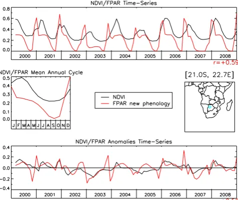
Fig. 1. Top plot: Monthly time series of the NDVI (black thick curve) and the FPAR (red thick curve) over the MODIS period, for a model box located in Bostwana (21.0◦S, 22.7◦E, see cyan diamond on the map). The correlation coefficient of the two time series is given on the right under the top plot (r=0.59). Using the nine years between 2000–2008, a mean annual cycle for both the NDVI and FPAR signals is derived (middle left plot). We then subtract each year these mean annual cycles from their respective time series and get NDVI and FPAR anomaly time series (bottom plot). The correlation coefficient of the two anomaly time series is given on the right under the bottom plot (r=0.52).
only the satellite pixels corresponding to this PFT. This pro-cedure results in a scoring for each of the 12 PFTs.
4 Illustrative results for a single simulation
4.1 Correlations at the model box level
An example of the methodology is shown at the model box level in Fig. 1. The plots are generated for a model box lo-cated in Botswana (see inset). The top figure shows the ob-served NDVI and the modeled FPAR for the ERA-I-based simulation with the new phenology version, over the nine-year period. Both time series show a clear annual cycle with vegetation growth towards the end of the year, and senes-cence around April (see the mean annual cycle). Although the agreement is not striking, there is some correspondence between the two time series. The correlation coefficient, (r),
Fig. 2. Correlation map between the NDVI and the FPAR monthly time series for the 2000–2008 period and the ERA-I simulation with the new phenology scheme. The correlation is not calculated when no annual cycle in the NDVI and FPAR is detected (grey areas).
4.2 Correlation map
The corresponding map of correlation coefficients is shown in Fig. 2. This particular figure was obtained based on the simulation forced by the ERA-Interim meteorology and the new phenology version of ORCHIDEE. The highest corre-lations (>0.8) are found over high temperate latitudes, es-pecially Europe and large parts of North America. There are also high correlations over tropical Raingreen Africa and Brazil. Approximately 10 % of the boxes do not exhibit a significant seasonal cycle, neither in the measurements nor in the model results. They are represented in grey in Fig. 2. These boxes are mostly located either over desert or in the tropical evergreen forest areas. Still, low correlations (close to zero) are found over equatorial forests (Amazonia, Cen-tral Africa, Indonesia), indicating a real model deficiency in these regions. A closer analysis of these latter regions shows that the satellite NDVI time series exhibits a significant an-nual cycle, while the modeled FPAR shows either no cycle or a phase-shifted one. Indeed, in Amazonia, a marked annual cycle has been observed over evergreen forests using MODIS Enhanced Vegetation Index (EVI; Huete et al., 2006; Moreau et al., 2010) or MODIS LAI (Myneni et al., 2007). LAI and EVI are preferred in these studies to FPAR and NDVI as they do not saturate over dense vegetation and then have larger amplitude (Huete et al., 2002). Hence, the extension of the grey zone could have been smaller if we have used EVI instead of NDVI. The failure of the ORCHIDEE veg-etation model over these regions needs to be further inves-tigated. As an example, the BIOME-BGC model has been shown to underestimate rooting depth in the Amazon, an important parameter because it controls water stress during the dry season, when plants have access to moisture only in deeper soil (Ichii et al., 2007). A similar deficiency in the ORCHIDEE model was recently shown when assimilating FLUXNET data to optimize the model parameters (Verbeeck et al., 2011). Furthermore, seasonal variations in leaf phe-nology for evergreen tropical forests are currently being in-troduced in ORCHIDEE (de Weirdt et al., 2010).
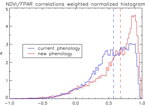
Fig. 3. NDVI/FPAR monthly correlations weighted histograms for the current phenology (blue curve) and for the new phenology (red curve) simulations, both forced by ERA-I fields (binsize=0.02). The vertical dashed lines indicate the weighted median values.
5 Application to the comparison of different simulations
We now discuss the application of the general methodology described in Sect. 3 to two sets of model versions. The first one focuses on a structural modification of the model phe-nology, while the second concerns the input meteorological fields.
5.1 Evaluation of the phenology modeling
Figure 3 shows the surface-weighted normalized histograms of two monthly correlation maps, in blue for the simula-tion with the current phenology and in red for the simu-lation with the new phenology modules. Both simusimu-lations are driven with the same ERA-Interim meteorology. A his-togram shifted to the right is desirable. The comparison of the two histograms clearly indicates that the new modeling of the phenology performs better; the surface-weighted me-dian value of the monthly correlations is 0.67 for the new phenology against 0.57 for the current one.
Fig. 4. Difference between the correlation maps for the new phe-nology and the current phephe-nology.
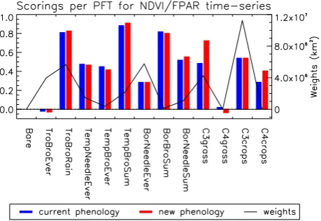
Fig. 5. Surface-weighted median values per PFT, for the NDVI/FPAR time series correlations. The blue bars are for the cur-rent phenology and the red bars for the new phenology. The black thick line indicates the total surface of the boxes used to assess the PFT median correlation.
impact of the structural model modification is not random but rather biome-dependent.
Figure 5 shows the surface-weighted median correlations for each of the 12 PFTs together with their respective sur-faces and for the two phenology schemes. Only the boxes where the specific PFT is dominant (>50 % fractional cover) are considered here. Figure 5 confirms that the ability of the model to reproduce the observed annual cycles strongly depends on the PFT. As already explained above, the Trop-ical Broad-leaved Evergreen PFT shows a poor correlation. The best score on the other hand is found for the Temperate Broad-leaved Summer-green PFT. Figure 5 shows that the improvement for the new phenology version is essentially for the C3 Grass PFT, with a weighted median correlation value of 0.72 rather than 0.48. The C4 Crop PFT also shows an improvement, but it describes a very small surface. There is no improvement for the C3 Crop PFT, which is surprising as some of the phenology modifications were targeted at this specific PFT.
This outcome thus needs to be analyzed more in detail. The correlation histograms for the C3 Crop PFT are shown
Fig. 6. Weighted normalized histograms of the correlations between the partial NDVI and partial FPAR for the PFT C3 Crops, in blue for the current phenology and in red for the new phenology (bin-size=0.02).
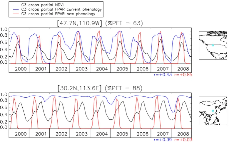
Fig. 7. Time series for two C3 Crops boxes located respectively in the Great Plains of North America (upper plot) and south-east of China (lower plot); NDVI is in black, the FPAR for the current phenology is in blue and the FPAR for the new phenology is in red. The plots give only the signals related to the C3 Crops fraction of the boxes. For the upper plot, the new phenology delivers a C3 Crops FPAR whose phasing with the C3 Crops NDVI has largely been improved (r=0.85), as compared to the C3 Crops FPAR of the current phenology (r=0.43). For the lower plot box, the C3 Crops NDVI exhibits a regular double cropping signal, the C3 Crops FPAR delivered by the new phenology is in phase with the first observed crop cycle but, as only one crop type is simulated, there is no modeled signal corresponding to the second observed crop cycle, thus resulting in an absence of correlation (r=0.03).
5.2 Evaluation of the meteorological forcings
We now evaluate the impact of using two different sets of global meteorological inputs. The procedure is similar as to the one above and we use the ORCHIDEE version with the new phenology scheme. When looking at the modeled time series over the same time frame against those of the satel-lite data, the weighted median values of the correlation are rather similar. The ERA-I forcing leads to a median value of r=0.67 while CRU-NCEP leads tor=0.66. The two different meteorology fields thus do not lead to significant global differences in the mean seasonal cycle generated by ORCHIDEE. We then compare the anomaly time series. Re-producing the interannual variations of leaf activity is more difficult than reproducing the mean annual cycle and, as ex-pected, the mean correlations are much lower than those ob-tained with the original time series. Although the model-measurement correspondence is poor, it is nevertheless sig-nificantly better (given the large number of grid boxes, more than 20 000) for the ERA-I forcing (r=0.25) than for the CRU-NCEP forcing (r=0.19). This result may indicate the better quality of the ERA-I re-analysis interannual sig-nal compared to CRU-NCEP, and the model ability to make use of it.
Fig. 8. Surface-weighted median values per PFT, for the anomaly NDVI/FPAR time series correlations. The green bars are for CRU-NCEP meteorological forcing and the red bars for ERA-Interim me-teorological forcing. The black thick line indicates the total surface of the boxes used to assess the PFT median correlation.
the vegetation maps are coherent. Hence a box is selected in each simulation only if the vegetation fraction of the domi-nant PFT is higher than 0.5 and if the domidomi-nant PFT of the nearest box of the other simulation is the same, and with a vegetation fraction higher than 0.5, even though Jung et al. (2007b) did not identify different land cover maps as a key factor for different outputs. This analysis per PFT con-firms that the ERA-I-based simulation reproduces the inter-annual variability better than the CRU-NCEP simulation for a majority of cases. This holds true for the Tropical Broad-leaved Raingreen PFT, for all three Temperate PFTs, and for the two C3 PFTs. There are no common boxes for the two C4 PFTs and the Boreal Broad-leaved Summer-green PFT. At face value CRU-NCEP leads to a better median correla-tion for the two Evergreen PFTs. The simulacorrela-tions perform similarly for the Boreal Needleleaf Summer-green.
We performed a similar study per season (December, January and February representing Winter in the Northern Hemisphere for example, and the seasons in the Southern Hemisphere with a six-month shift). We found that Spring gives the best scorings for the modeled FPAR anomaly time series, which is expected as the onset is very sensitive to climate modifications, at least in the northern mid-latitudes (Schwartz et al., 2006; Richardson et al., 2010). The best scorings are for the C3 Crop PFT (r=0.54 for ERA-I) and the Boreal Needleleaf Summer-green (r=0.37 for CRU-NCEP). There is no significant difference between seasons, so that no specific season drives the better scoring of ERA-I for anomaly time series.
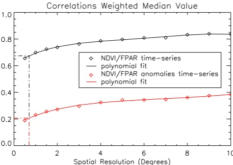
5.3 Impact of the spatial resolution
We now study how the satellite NDVI versus modeled FPAR correlation is sensitive to the spatial resolution. For this ob-jective, we used the CRU-NCEP simulation as its regular 0.5◦grid is easier to handle than the irregular ERA-I Gaus-sian grid, and can be degraded through a simple averaging. Figure 9 shows the median correlations for both the time se-ries and their interannual anomalies for a spatial resolution of 0.5◦to 10◦; the model-observation correspondence increases as the spatial resolution gets coarser. A simple explanation is that spatial averaging decreases the non systematic errors. Such random errors are certainly present in the satellite data. They may also be present in the model results, in particu-lar due to random errors in the meteorological forcing. The significant improvement in the correlation with coarser reso-lution puts our earlier result on the better performance of the ERA-I forcing compared to that of CRU-NCEP into ques-tion. Indeed, the ERA-I analysis has a resolution of 0.7◦, against 0.5◦for that of CRU-NCEP, and one may therefore question whether the comparison is fair. From the data points shown in Fig. 9, we performed a simple polynomial fit and used the fit to extrapolate the CRU-NCEP results to a hypo-thetical resolution of 0.7◦ (vertical dashed lines in Fig. 9). The interpolated correlations are 0.67 for the time series and
Fig. 9. Surface-weighted median values for the NDVI/FPAR time series (thick black diamonds) and anomaly time series correlations (thick red diamonds), as a function of the spatial resolution. The black and red curves are the results of degree 5 polynomial fit. The dashed lines indicate the extrapolation to the theoretical resolution of 0.7◦using the polynomial fit.
0.21 for the anomalies, which is still statistically significantly lower than the 0.25 value obtained with the ERA-I forcing.
Therefore, although the spatial resolution may explain some of the better results obtained with the ERA-I meteo-rological fields, it cannot explain them fully, and the data of the latter are most likely of better quality, in particular when considering the interannual variations.
6 Discussion and conclusions
This work demonstrates a global satellite database can be used to rank several versions of the ORCHIDEE model. Evaluations of DGVMs using satellite data have been pub-lished before, but not using the spatial and temporal resolu-tion of the present study. For instance, Krinner et al. (2005) focused on the mean LAI over a 5 yr period at coarse scale (4◦×2.5◦). Other studies (e.g. Kim and Wang, 2005; Twine and Kucharik, 2008) focused over North America and did not analyze all biomes. To our knowledge, there is no previ-ously published work that compares the annual cycle and the interannual anomalies of the model outputs and the satellite observations.
We observed no significant trends over the nine year-period of the study, neither in the satellite data nor in the modeled FPAR. When the weekly temporal resolution was available for the outputs (for the ERA-I simulations) we found a slightly lesser weighted median value than for the monthly resolution (e.g. 0.65 against 0.67, for the second simulation with the new phenology). We tested other ex-tinction coefficient values for the FPAR/LAI relationship (Eq. 1), as mentioned in Beer et al. (2009): 0.7 for Decid-uous Broad-leaved forests, including PFTs 3, 6 and 8 and 0.4 for grasses, including PFTs 12 and 13. This modifica-tion had only a small impact on the time series correlamodifica-tions with a final scoring for the corresponding PFTs changing by less than 0.02. When comparing the simulations per PFT we adopted a rather conservative approach by imposing a mini-mum threshold of 0.5 on the PFT fractional cover for a box to be considered. This was done to be sure that there was enough information in the NDVI signal for the correspond-ing PFT. However it is worth notcorrespond-ing that even when lowercorrespond-ing this threshold to 0.2, the median correlations are degraded by less than−0.01 on the average.
The comparison of the model outputs with the satellite data produces a very wide range of correlations for the C3 Crop PFT. This is most likely due to the fact that C3 crops are very diverse, with different phenologies and different agri-culture practices. This work stresses the necessity to split the Crop PFTs between several crop types (maybe first by sim-ply regionalizing the PFTs parameter values) to get realistic simulated seasonal cycles all over the world.
The present study demonstrates the possibility of using satellite data as an objective means to evaluate the perfor-mance of various versions of the ORCHIDEE model. It could of course be also applied to other DGVMs, or for inter-model evaluations. In the future we will systematically perform a similar evaluation for each new version of the ORCHIDEE model. The next planned new functionalities will concern the nitrogen cycle (Zaehle et al., 2010), and the introduction of specific crop modules (Gervois et al., 2008). We will also test EVI instead of NDVI in our procedure, as this variable appears to be quite robust to atmospheric conditions over the tropical forests (Poulter and Cramer, 2009).
Supplementary material related to this article is available online at:
http://www.geosci-model-dev.net/4/1103/2011/ gmd-4-1103-2011-supplement.pdf.
Acknowledgements. This study has been co-funded by the Eu-ropean Commission under the EU Seventh Research Framework Programme (grant agreement No. 218795, GEOLAND2). The authors thank Benjamin Poulter and Natasha MacBean for their useful suggestions.
Edited by: D. Lawrence
The publication of this article is financed by CNRS-INSU.
References
Abramowitz, G.: Towards a benchmark for land surface models, Geophys. Res. Lett., 32, L22702, doi:10.1029/2005gl024419, 2005.
Beer, C., Ciais, P., Reichstein, M., Baldocchi, D., Law, B. E., Pa-pale, D., Soussana, J. F., Ammann, C., Buchmann, N., Frank, D., Gianelle, D., Janssens, I. A., Knohl, A., Kostner, B., Moors, E., Roupsard, O., Verbeeck, H., Vesala, T., Williams, C. A., and Wohlfahrt, G.: Temporal and among-site variability of inherent water use efficiency at the ecosystem level, Global Biogeochem. Cy., 23, Gb2018, doi:10.1029/2008gb003233, 2009.
Berrisford, P., Dee, D., Fielding, K., Fuentes, M., Kallberg, P., Kobayashi, S., and Uppala, S.: The Interim archive, ERA-40 Report Series N◦1, ECMWF, Shinfield Park, Reading, 2009. Blyth, E., Clark, D. B., Ellis, R., Huntingford, C., Los, S., Pryor,
M., Best, M., and Sitch, S.: A comprehensive set of benchmark tests for a land surface model of simultaneous fluxes of water and carbon at both the global and seasonal scale, Geosci. Model Dev., 4, 255–269, doi:10.5194/gmd-4-255-2011, 2011.
Bonan, G. B. and Levis, S.: Evaluating aspects of the community land and atmosphere models (clm3 and cam3) using a dynamic global vegetation model, J. Climate, 19, 2290–2301, 2006. Bondeau, A., Smith, P. C., Zaehle, S., Schaphoff, S., Lucht,
W., Cramer, W., and Gerten, D.: Modelling the role of agriculture for the 20th century global terrestrial carbon bal-ance, Glob. Change Biol., 13, 679–706, doi10.1111/j.1365-2486.2006.01305.x, 2007.
Botta, A., Viovy, N., Ciais, P., Friedlingstein, P., and Monfray, P.: A global prognostic scheme of leaf onset using satellite data, Glob. Change Biol., 6, 709–725, 2000.
Cadule, P., Friedlingstein, P., Bopp, L., Sitch, S., Jones, C. D., Ciais, P., Piao, S. L., and Peylin, P.: Benchmarking coupled climate-carbon models against long-term atmospheric CO2 measurements, Global Biogeochem. Cy., 24, Gb2016, doi:10.1029/2009gb003556, 2010.
Chuine, I.: A unified model for budburst of trees, J. Theor. Biol., 207, 337–347, 2000.
Ciais, P., Reichstein, M., Viovy, N., Granier, A., Ogee, J., Al-lard, V., Aubinet, M., Buchmann, N., Bernhofer, C., Carrara, A., Chevallier, F., De Noblet, N., Friend, A. D., Friedlingstein, P., Grunwald, T., Heinesch, B., Keronen, P., Knohl, A., Krin-ner, G., Loustau, D., Manca, G., Matteucci, G., Miglietta, F., Ourcival, J. M., Papale, D., Pilegaard, K., Rambal, S., Seufert, G., Soussana, J. F., Sanz, M. J., Schulze, E. D., Vesala, T., and Valentini, R.: Europe-wide reduction in primary productivity caused by the heat and drought in 2003, Nature, 437, 529–533, doi:10.1038/Nature03972, 2005.
feedbacks in a coupled climate model (vol 408, pg 184, 2000), Nature, 408, 750–750, 2000.
Cramer, C.: Biome Models, Volume 2, The Earth system: biolog-ical and ecologbiolog-ical dimensions of global environmental change, in: Encyclopedia of Global Environmental Change, edited by: Mooney, H. A. and Canadell, J. G., Editor-in-Chief Ted Munn, John Wiley & Sons, Ltd, Chichester, 166–171, (ISBN 0-471-97796-9), 2002.
de Weirdt, M., Verbeeck, H., Maignan, F., Moreau, I., Defourny, P., and Steppe, K.: Modelling the foliage seasonal carbon cycle in tropical forests, Proceedings of the ESA-iLEAPS-EGU Earth Observation for Land-Atmosphere Interaction Science Confer-ence, 3–5 November 2010, Frascati (Rome), Italy, 2010. Friedlingstein, P., Cox, P., Betts, R., Bopp, L., Von Bloh, W.,
Brovkin, V., Cadule, P., Doney, S., Eby, M., Fung, I., Bala, G., John, J., Jones, C., Joos, F., Kato, T., Kawamiya, M., Knorr, W., Lindsay, K., Matthews, H. D., Raddatz, T., Rayner, P., Re-ick, C., Roeckner, E., Schnitzler, K. G., Schnur, R., Strassmann, K., Weaver, A. J., Yoshikawa, C., and Zeng, N.: Climate-carbon cycle feedback analysis: Results from the (cmip)-m-4 model in-tercomparison, J. Climate, 19, 3337–3353, 2006.
Gervois, S., Ciais, P., de Noblet-Ducoudre, N., Brisson, N., Vuichard, N., and Viovy, N.: Carbon and water balance of euro-pean croplands throughout the 20th century, Global Biogeochem. Cy., 22, Gb2022, doi:10.1029/2007gb003018, 2008.
Gulden, L. E., Rosero, E., Yang, Z. L., Wagener, T., and Niu, G. Y.: Model performance, model robustness, and model fitness scores: A new method for identifying good land-surface, Geophys. Res. Lett., 35, L11404, doi10.1029/2008gl033721, 2008.
Hansen, M. C., Defries, R. S., Townshend, J. R. G., and Sohlberg, R.: Global land cover classification at 1km spatial resolution us-ing a classification tree approach, Int. J. Remote Sens., 21, 1331– 1364, 2000.
Heymann Y., Steenmans, C., Croisille, G., Bossard, M., Lenco, M., Wyatt, B., Weber, J.-L., O’Brian, C., Cornaert, M.-H., and Sifakis, N.: CORINE Land Cover: Technical Guide. Environ-ment, nuclear safety and civil protection series, Commission of the European Communities, Office for Official Publications of the European Communities, Luxembourg, EUR 12585, 144 pp., (English version: ISBN 92-826-2578-8, French version: ISBN 92-826-2579-6), 1993.
Huete, A., Didan, K., Miura, T., Rodriguez, E. P., Gao, X., and Fer-reira, L. G.: Overview of the radiometric and biophysical perfor-mance of the modis vegetation indices, Remote Sens. Environ., 83, 195–213, 2002.
Huete, A. R., Didan, K., Shimabukuro, Y. E., Ratana, P., Saleska, S. R., Hutyra, L. R., Yang, W. Z., Nemani, R. R., and Myneni, R.: Amazon rainforests green-up with sunlight in dry season, Geo-phys. Res. Lett., 33, L06405, doi:10.1029/2005gl025583, 2006. Ichii, K., Hashimoto, H., White, M. A., Potters, C., Hutyra, L.
R., Huete, A. R., Myneni, R. B., and Nemanis, R. R.: Con-straining rooting depths in tropical rainforests using satellite data and ecosystem modeling for accurate simulation of gross pri-mary production seasonality, Glob. Change Biol., 13, 67–77, doi:10.1111/j.1365-2486.2006.01277.x, 2007.
IPCC: Climate Change 2007: The Physical Science Basis, Con-tribution of Working Group I to the Fourth Assessment, Report of the Intergovernmental Panel on Climate Change, edited by: Solomon, S., Qin, D., Manning, M., Chen, Z., Marquis, M.,
Av-eryt, K. B., Tignor. M., and Miller, H. L., Cambridge University Press, Cambridge, United Kingdom and New York, NY, USA, 996 pp., 2007.
Jung, M., Le Maire, G., Zaehle, S., Luyssaert, S., Vetter, M., Churk-ina, G., Ciais, P., Viovy, N., and Reichstein, M.: Assessing the ability of three land ecosystem models to simulate gross carbon uptake of forests from boreal to Mediterranean climate in Eu-rope, Biogeosciences, 4, 647–656, doi:10.5194/bg-4-647-2007, 2007a.
Jung, M., Vetter, M., Herold, M., Churkina, G., Reichstein, M., Zaehle, S., Ciais, P., Viovy, N., Bondeau, A., Chen, Y., Trusilova, K., Feser, F., and Heimann, M.: Uncertainties of modeling gross primary productivity over europe: A system-atic study on the effects of using different drivers and terres-trial biosphere models, Global Biogeochem. Cy., 21, Gb4021, doi:10.1029/2006gb002915, 2007b.
Kalnay, E., Kanamitsu, M., Kistler, R., Collins, W., Deaven, D., Gandin, L., Iredell, M., Saha, S., White, G., Woollen, J., Zhu, Y., Chelliah, M., Ebisuzaki, W., Higgins, W., Janowiak, J., Mo, K. C., Ropelewski, C., Wang, J., Leetmaa, A., Reynolds, R., Jenne, R., and Joseph, D.: The ncep/ncar 40-year reanalysis project, B. Am. Meteorol. Soc., 77, 437–471, 1996.
Kim, Y. and Wang, G. L.: Modeling seasonal vegetation variation and its validation against moderate resolution imaging spectrora-diometer (modis) observations over north america, J. Geophys. Res.-Atmos., 110, D04106, doi:10.1029/2004jd005436, 2005. Krinner, G., Viovy, N., de Noblet-Ducoudre, N., Ogee, J., Polcher,
J., Friedlingstein, P., Ciais, P., Sitch, S., and Prentice, I. C.: A dynamic global vegetation model for studies of the cou-pled atmosphere-biosphere system, Global Biogeochem. Cy., 19, Gb1015, doi:10.1029/2003gb002199, 2005.
Mitchell, T. D. and Jones, P. D.: An improved method of con-structing a database of monthly climate observations and as-sociated high-resolution grids, Int. J. Climatol., 25, 693–712, doi:10.1002/Joc.1181, 2005.
Monsi, M. and Saeki, T.: ¨Uber den Lichtfaktor in den Planzenge-sellshaften und seine Bedeutung f¨ur die Stoffproducktion, Jpn J. Bot., 14, 22–52, 1953.
Moreau, I., Defourny P., Hanert, E., de Weirdt, M., Verbeeck, H., and Steppe, K.: Integrating SPOT-GVT 10-y time series to fore-cast terrestrial carbon dynamics: The vegetation phenology de-tection in tropical evergreen forests. Proceedings of the ESA-iLEAPS-EGU Earth Observation for Land-Atmosphere Interac-tion Science Conference, 3–5 November 2010, Frascati (Rome), Italy, 2010.
Mueller, B., Seneviratne, S. I., Jimenez, C., Corti, T., Hirschi, M., Balsamo, G., Ciais, P., Dirmeyer, P., Fisher, J. B., Guo, Z., Jung, M., Maignan, F., McCabe, M. F., Reichle, R., Reichstein, M., Rodell, M., Sheffield, J., Teuling, A. J., Wang, K., Wood, E. F., and Zhang, Y.: Evaluation of global observations-based evap-otranspiration datasets and ipcc ar4 simulations, Geophys. Res. Lett., 38, L06402, doi:10.1029/2010gl046230, 2011.
D. P., Wolfe, R. E., Friedl, M. A., Running, S. W., Votava, P., El-Saleous, N., Devadiga, S., Su, Y., and Salomonson, V. V.: Large seasonal swings in leaf area of amazon rainforests, Proc. Nat. Ac. Sci. USA, 104, 4820–4823, doi:10.1073/pnas.0611338104, 2007.
Piao, S. L., Ciais, P., Friedlingstein, P., Peylin, P., Reichstein, M., Luyssaert, S., Margolis, H., Fang, J. Y., Barr, A., Chen, A. P., Grelle, A., Hollinger, D. Y., Laurila, T., Lindroth, A., Richard-son, A. D., and Vesala, T.: Net carbon dioxide losses of northern ecosystems in response to autumn warming, Nature, 451, 49–52, doi:10.1038/Nature06444, 2008.
Piao, S. L., Ciais, P., Huang, Y., Shen, Z. H., Peng, S. S., Li, J. S., Zhou, L. P., Liu, H. Y., Ma, Y. C., Ding, Y. H., Friedlingstein, P., Liu, C. Z., Tan, K., Yu, Y. Q., Zhang, T. Y., and Fang, J. Y.: The impacts of climate change on water resources and agriculture in china, Nature, 467, 43–51, doi:10.1038/Nature09364, 2010. Poulter, B. and Cramer, W.: Satellite remote sensing of tropical
forest canopies and their seasonal dynamics, Int. J. Remote Sens., 30, 6575–6590, doi:10.1080/01431160903242005, 2009. Prentice, I. C., Cramer, W., Harrison, S. P., Leemans, R., Monserud,
R. A., and Solomon, A. M.: A global biome model based on plant physiology and dominance, soil properties and climate, J. Biogeogr., 19, 117–134, 1992.
Randerson, J. T., Hoffman, F. M., Thornton, P. E., Mahowald, N. M., Lindsay, K., Lee, Y. H., Nevison, C. D., Doney, S. C., Bo-nan, G., Stockli, R., Covey, C., Running, S. W., and Fung, I. Y.: Systematic assessment of terrestrial biogeochemistry in cou-pled climate-carbon models, Glob. Change Biol., 15, 2462–2484, doi:10.1111/j.1365-2486.2009.01912.x, 2009.
Ratel, G.: Median and weighted median as estimators for the key comparison reference value (kcrv), Metrologia, 43, S244–S248, doi:10.1088/0026-1394/43/4/S11, 2006.
Richardson, A. D., Black, T. A., Ciais, P., Delbart, N., Friedl, M. A., Gobron, N., Hollinger, D. Y., Kutsch, W. L., Longdoz, B., Luyssaert, S., Migliavacca, M., Montagnani, L., Munger, J. W., Moors, E., Piao, S. L., Rebmann, C., Reichstein, M., Saigusa, N., Tomelleri, E., Vargas, R., and Varlagin, A.: Influence of spring and autumn phenological transitions on forest ecosystem produc-tivity, Phil. Trans. Roy. Soc. B-Biological Sciences, 365, 3227– 3246, doi:10.1098/rstb.2010.0102, 2010.
Running, S. W.: Is global warming causing more, larger wildfires?, Science, 313, 927–928, doi:10.1126/science.1130370, 2006. Schwartz, M. D., Ahas, R., and Aasa, A.: Onset of spring starting
earlier across the northern hemisphere, Glob. Change Biol., 12, 343–351, doi:10.1111/j.1365-2486.2005.01097.x, 2006. Seneviratne, S., Ciais, P., Reichstein, M., Davin, E.L., Orlowsky,
B., and Teuling, A. J.: Using observational diagnostics of soil moisture-climate interactions as constraints to IPCC climate pro-jections, Proceedings of the 6th International Scientific Confer-ence on the Global Energy and Water Cycle and 2nd Integrated Land Ecosystem – Atmosphere Processes Study (iLEAPS) Sci-ence ConferSci-ence, 24–28 August 2009, Melbourne, Australia, Volume I, 2009.
Tucker, C. J.: Red and photographic infrared linear combinations for monitoring vegetation, Remote Sens. Environ., 8, 127–150, 1979.
Twine, T. E. and Kucharik, C. J.: Evaluating a terrestrial ecosystem model with satellite information of greenness, J. Geophys. Res.-Biogeosci., 113, G03027, doi:10.1029/2007jg000599, 2008. Verbeeck, H., Peylin, P., Bacour, C., Bonal, D., Steppe, K. and Ciais
P.: Seasonal patterns of CO2fluxes in Amazon forests: fusion of eddy covariance data and the ORCHIDEE model, J. Geophys. Res.-Biogeosci., 116, G02018, doi:10.1029/2010JG001544, 2011.
Vermote, E. F., El Saleous, N. Z., and Justice, C. O.: Atmospheric correction of modis data in the visible to middle infrared: First results, Remote Sens. Environ., 83, 97–111, 2002.
Vermote, E., Justice, C. O., and Breon, F. M.: Towards a gener-alized approach for correction of the brdf effect in modis direc-tional reflectances, Ieee Trans. Geosci. Remote Sens., 47, 898– 908, doi:10.1109/Tgrs.2008.2005977, 2009.
Zaehle, S., Friend, A. D., Friedlingstein, P., Dentener, F., Peylin, P., and Schulz, M.: Carbon and nitrogen cycle dynamics in the o-cn land surface model: 2. Role of the nitrogen cycle in the historical terrestrial carbon balance, Global Biogeochem. Cy., 24, Gb1006, doi:10.1029/2009gb003522, 2010.