Contribution of emissions to concentrations: the TAGGING 1.0 submodel based on the Modular Earth Submodel System (MESSy 2.52)

https://doi.org/10.5194/gmd-10-2615-2017 © Author(s) 2017. This work is distributed under the Creative Commons Attribution 3.0 License.

Contribution of emissions to concentrations: the TAGGING 1.0

submodel based on the Modular Earth Submodel

System (MESSy 2.52)

Volker Grewe1,2, Eleni Tsati1, Mariano Mertens1, Christine Frömming1, and Patrick Jöckel1

1_{Deutsches Zentrum für Luft- und Raumfahrt, Institut für Physik der Atmosphäre, Oberpfaffenhofen, Germany}

2_{Delft University of Technology, Aerospace Engineering, Section Aircraft Noise and Climate Effects, Delft, the Netherlands} Correspondence to:Volker Grewe ([email protected])

Received: 6 December 2016 – Discussion started: 5 January 2017 Revised: 2 May 2017 – Accepted: 7 June 2017 – Published: 10 July 2017

Abstract.Questions such as “what is the contribution of road traffic emissions to climate change?” or “what is the im-pact of shipping emissions on local air quality?” require a quantification of the contribution of specific emissions sec-tors to the concentration of radiatively active species and air-quality-related species, respectively. Here, we present a di-agnostics package, implemented in the Modular Earth Sub-model System (MESSy), which keeps track of the contri-bution of source categories (mainly emission sectors) to various concentrations. The diagnostics package is imple-mented as a submodel (TAGGING) of EMAC (European Centre for Medium-Range Weather Forecasts – Hamburg (ECHAM)/MESSy Atmospheric Chemistry). It determines the contributions of 10 different source categories to the con-centration of ozone, nitrogen oxides, peroxyacytyl nitrate, carbon monoxide, non-methane hydrocarbons, hydroxyl, and hydroperoxyl radicals (=tagged tracers). The source cate-gories are mainly emission sectors and some other sources for completeness. As emission sectors, road traffic, shipping, air traffic, anthropogenic non-traffic, biogenic, biomass burn-ing, and lightning are considered. The submodel obtains in-formation on the chemical reaction rates, online emissions, such as lightning, and wash-out rates. It then solves differ-ential equations for the contribution of a source category to each of the seven tracers. This diagnostics package does not feed back to any other part of the model. For the first time, it takes into account chemically competing effects: for ex-ample, the competition between NOx, CO, and non-methane

hydrocarbons (NMHCs) in the production and destruction of ozone. We show that the results are in-line with results from

other tagging schemes and provide plausibility checks for concentrations of trace gases, such as OH and HO2, which

have not previously been tagged. The budgets of the tagged tracers, i.e. the contribution from individual source categories (mainly emission sectors) to, e.g., ozone, are only marginally sensitive to changes in model resolution, though the level of detail increases. A reduction in road traffic emissions by 5 % shows that road traffic global tropospheric ozone is reduced by 4 % only, because the net ozone productivity increases. This 4 % reduction in road traffic tropospheric ozone corre-sponds to a reduction in total tropospheric ozone by≈0.3 %, which is compensated by an increase in tropospheric ozone from other sources by 0.1 %, resulting in a reduction in to-tal tropospheric ozone of≈0.2 %. This compensating effect compares well with previous findings. The computational costs of the TAGGING submodel are low with respect to computing time, but a large number of additional tracers are required. The advantage of the tagging scheme is that in one simulation and at every time step and grid point, information is available on the contribution of different emission sectors to the ozone budget, which then can be further used in up-coming studies to calculate the respective radiative forcing simultaneously.

1 Introduction

Nitrogen oxides (NOx), carbon monoxide (CO), methane

(CH4), and non-methane hydrocarbons (NMHCs) are

con-tribution of individual emissions of these precursors on air quality and climate requires a detailed analysis of the chem-ical conversion, transport, and deposition of these species in numerical atmosphere–chemistry simulations. A frequently used method is called “tagging” (Horowitz and Jacob, 1999; Lelieveld and Dentener, 2000; Meijer et al., 2000; Dunker et al., 2002; Grewe, 2004; Gromov et al., 2010; Butler et al., 2011; Emmons et al., 2012; Grewe et al., 2012). Technically, this method adds a set of diagnostic tracers for each chemi-cal species or chemichemi-cal family considered, i.e. one additional tracer per source category for each chemical species or fam-ily considered. For example, for the famfam-ily of reactive nitro-gen compounds NOy, a set of tagged tracers NOanty , NOrty,

NOshpy , NOairy , NObioy , NObby , NO lig

y , NOCHy 4, NONy2O, and

NOstr_y is added, which describes the NOyconcentration from

anthropogenic non-traffic (e.g. industry, households), road traffic, ships, air traffic, biogenic, biomass burning, lightning, methane and nitrous oxide decomposition, and stratospheric ozone production. The idea is that these tagged tracers ex-perience the same chemical conversions, sources, and loss processes (such as deposition) as the simulated tracer NOy.

If all emissions of NOy are considered and tagged, the sum

of all tagged diagnostic NOy tracers equals the simulated

NOytracer in this approach. A full partition of the simulated

tracer concentration with respect to emission sectors can be achieved. Thus, the contribution of an emission sector, such as industry, road traffic, etc., to a concentration is provided by the tagging method.

The abundances of carbon compounds (CO, CH4,

NMHCs) and nitrogen oxides are both limiting factors for tropospheric ozone production (Sillman, 1995). Many tag-ging mechanisms for global applications concentrate on NOx

compounds (Horowitz and Jacob, 1999; Lelieveld and Den-tener, 2000; Meijer et al., 2000; Grewe, 2004; Grewe et al., 2012) only. Butler et al. (2011) tags the sources for hydro-gen carbons. Dunker et al. (2002) tags ozone sensitivities and attributes them to either nitrogen oxides or volatile organic compounds (VOCs) depending on the chemical regime. This latter mechanism is a very helpful tool in understanding the underlying chemical processes and especially sensitivities. However, the mechanism differs in principle from other tag-ging mechanisms. One consequence is that the sum of all contributions is not adding up to the ozone concentration. The focus on the ozone sensitivities makes that scheme more similar to the perturbation approach.

This perturbation approach (e.g. Hoor et al., 2009; Grewe et al., 2007, and many others), where results from two simu-lations are compared that differ in the strength of an individ-ual emission source, identify the impact of changes in emis-sions (e.g. by mitigation options) on the atmospheric com-position. It is important not to confuse both approaches. For example, the change in ozone due to a 100 % reduction in road traffic emissions is smaller by a factor of 5 than the con-tribution of the road traffic emissions to ozone (Grewe et al.,

2012). Emmons et al. (2012) showed that similar results (fac-tor of 3) are obtained for biomass burning NOx emissions

and the impact on ozone. Clearly, the non-linearity in the ozone chemistry leads to these large differences. Any reduc-tion in NOxemission leads mostly to a larger ozone

produc-tion efficiency. Grewe et al. (2012) showed that in the simu-lation without road traffic NOxemissions, the obvious large

reduction in ozone from the reduced road traffic contribution to ozone is compensated by larger contributions from other emission sectors, not because these emissions are changed, but because the ozone production efficiency is increased.

These two different approaches answer two different ques-tions. The perturbation approach quantifies how much a con-centration changes if emissions are changed, whereas tag-ging addresses the contribution of an emission to the concen-tration. The combination of both approaches leads to much better insights in the reasons how emission changes lead to concentration changes (Grewe et al., 2012). Note also that the perturbation approach often requires the identical meteorol-ogy in either simulation to enhance the signal-to-noise ratio enabling a robust signal. However, this is not feasible in fully coupled chemistry–climate models unless run in a “QCTM-mode”, which replaces instantaneous chemical feedbacks by climatological values (Deckert et al., 2011, see also below).

Most tagging approaches address a straight process chain from the emission of, e.g., NOx to a concentration of,

e.g., ozone. Grewe et al. (2010), as well as Grewe (2013a) and Tsati (2014), proposed a more general tagging approach, where competing mechanisms in the production of ozone can be taken into account; e.g. both NOxand carbon compounds

(CO, CH4, NMHCs) are precursors of ozone. This more

gen-eral tagging approach allows the contribution of road traffic NOx, CO, and NMHC emissions to ozone, for example, to

be determined. This generalised method has also been suc-cessfully applied to a non-chemical application, namely tem-perature in an energy balance model (Grewe, 2013b).

Here, we present a submodel (TAGGING) of an Earth sys-tem model (EMAC – European Centre for Medium-Range Weather Forecasts – Hamburg (ECHAM)/MESSy Atmo-spheric Chemistry), which applies this general tagging ap-proach to allow the contribution of NOx, CO, and NMHC

emissions from a variety of emission sectors to ozone and HOx chemistry to be quantified. Hence, it combines NOx

-ozone tagging approaches (Emmons et al., 2012) with VOC-ozone tagging approaches (Butler et al., 2011). In Sect. 2 we present the basic equations of the tagging scheme, whereas in Sect. 3 we present what emissions are addressed and how the tagging method is implemented. In Sect. 4 we show results of a base simulation and compare them with other modelling studies. Since no measurements are available for contribu-tions of emissions to ozone concentracontribu-tions, a direct compari-son with observational data is not possible. Instead, we show that the results are in agreement with other studies. Since the tagging of HOx components is new, we discuss those

and shipping emissions. Finally, we address sensitivities of the methodology (Sect. 5), with respect to the resolution and emission changes, and provide a comparison of the perturba-tion and tagging method.

2 Basics on tagging

The tagging approach that we adopt here is based on Grewe et al. (2010) and Grewe (2013a). We first describe the ba-sic mechanism and describe in Sect. 3 how this mechanism is applied in the submodel TAGGING. Exemplarily, we con-centrate on the main reaction for tropospheric ozone produc-tion:

NO+HO2−→NO2+OH. (R1)

Note, this reaction is not producing any ozone, but NO2 is

photolysed and recombines with O2to form ozone and

Reac-tion (R1) is the rate limiting step for this chain of reacReac-tions. The ozone production rate PR1 depends on the abundance

of NO and HO2, and the reaction rate coefficientkR1

(Re-action R1). The NO concentration in turn depends on emis-sions of NO from different emission sectors (here N in to-tal), such as industry and road traffic with the respective con-centration NOind_x and NOrt_x. Thus, the ozone production rate PR1has to be distributed to the sectors: industry, road traffic,

etc. This is achieved by a combinatoric redistribution accord-ing to the concentrations of the tagged family and species of NOx and HO2, respectively. Note that a full description of

the applied TAGGING mechanism, including the tagging of OH and HO2, is given in the next section. This means that

all possible combinations between a tagged NOxspecies and

another tagged HO2species are evaluated and its probability

calculated consistently with the calculation of the chemical production ratePR1. This is just a full partitioning of the

pro-duction ratePR1Grewe et al. (following 2010):

PR1=kR1NO HO2, (1)

=kR1 N

X

i=1

NOi

N

X

j=1

HO2j, (2)

=kR1 N

X

i=1

NOi HO2i+

X

j6=i

1 2NO

i _HOj

2 (3)

+X

j6=i

1 2NO

j_HO 2i

!

,

=

N

X

i=1

1 2kR1

NOi NO +

HO2i

HO2

!

, (4)

=

N

X

i=1

P_R1i . (5)

Hereiandj represent a counter for allN source categories; we have chosenN=10 source categories (see Sect. 3). The

factor 1₂ stems from the split of the part of the ozone pro-ductionkR1NOi HO2j(i6=j), which is equally attributed to

emission categoryiandj. Note that no approximation, lin-earisation, or Taylor approximation is used in this approach. For the ozone production due to NOxfrom industry (NOindx )

and due to HOind₂ from industry we hence obtain:

P_R1ind=PR1

1 2

NOind

NO +

HOind₂ HO2

!

. (6)

Note that this includes the reactions of NOind_x with all other HO2molecules and vice versa HOind₂ with other NOx

molecules without any double counting. The relevant differ-ential equation for the tagged species is then

d dtO

ind

3 =Pind−Dind, (7)

where Pind and Dind are the sum of all relevant produc-tion and loss terms. With this approach, Grewe et al. (2010) showed that the sum of all emissions contributions adds up to the total concentration of the respective species. For example, the ozone field is completely partitioned into emission sector contributions, if all emission sectors are included, leading to

N

X

i=1

O3i=O3. (8)

Note that the factor 0.5 in Eq. (6) is a result of the com-binatorical ansatz and not an assumption. It reflects that in Reaction (R1) both species are required and similar to the re-action rate coefficient it constitutes a basic principle. This should not be confused with effects of different chemical regimes on the ozone productivity, which are reflected in the concentrations of ozone and the tagged ozone fields. For example, when increasing NOx emissions in a

VOC-limited regime (i.e. any changes in nitrogen oxide emissions hardly change the ozone production), the ozone productivity or sensitivity attributed to NOx will decrease, whereas that

of VOCs remains unchanged.

This approach is identical to a different formulation, which describes the right-hand side of the differential equation more generally as the relative sensitivity of the individual production and loss terms with respect to the emission sector considered (Grewe, 2013a):

P_R1ind=PR1

SindT ∇_SPR1 ST ∇_SPR1

, (9)

whereSis the vector of all chemical compounds, e.g. ST =(NOx,CO,NMHC,O3, . . .)T,and (10) SindT =(NOind_x ,COind,NMHCind,O3ind, . . .)T, (11)

∇_SPR1=

d

dSPR1, (12)

providing two different interpretations of the differential Eq. (7).

To summarise, this tagging approach fully partitions in-dividual chemical fields into the contribution of inin-dividual emission sectors. There is no linearisation required and the approach utilises the identical chemical parameterisation as the underlying chemical scheme, with respect to the prob-ability that a reaction occurs. Note that the new aspect of this tagging approach compared to other tagging approaches (Grewe, 2007; Lelieveld and Dentener, 2000; Emmons et al., 2012) is the competing effect of NOxand carbon compounds

in producing ozone. Since the differential equation for the tagging Eq. (7) fully relies on the reaction rates and concen-trations, the tagging scheme can be implemented indepen-dently from the main chemical solver. However, details on many reaction rates have to be transferred from the chemical solver to the tagging scheme.

In the following, and actually this also applies to the pre-vious sections, we use the wording “contribution of emis-sions from a sector X to the atmospheric concentration of species (or family)Y”, when we are referring to that part of the concentrationY, which can be attributed to the emission sectorX, by a decomposition of the chemical reactions (see above). This implies that no changes in chemical reaction rates are assumed, e.g. for natural and anthropogenic emis-sions, which would represent different atmospheric situations for pre-industrial and today’s atmospheric chemical regimes. Obviously, other authors may have other definitions for this wording.

3 Implementation in EMAC/MECO(n)

The objective of the implementation of this tagging scheme is to be able to monitor online, i.e. at every model’s time step, the contribution of individual emission sectors to ozone and OH, allowing for a competition between ozone precursors, linearisation to be avoided, and applicable in decadal sim-ulations. The tagging approach requires one to quantify all sources of the species considered. Therefore, in addition to the emission sectors considered, there are additional source categories considered, such as ozone produced by photolysis of oxygen, which predominantly occurs in the stratosphere and which we therefore name stratospheric ozone produc-tion. Note that also in the upper troposphere, ozone is pro-duced by this reaction. In the following the base models are described for which the tagging scheme is developed, an overview on the tagging scheme is given, and the tagging chemistry is described.

3.1 Description of MESSy, EMAC, and MECO(n)

The TAGGING model described here (see also Tsati, 2014) is written as a submodel of the Modular Earth Submodel

System (MESSy), which comprises a standard interface to couple different processes, a simple coding standard and a set of different submodels (Jöckel et al., 2005). The TAG-GING submodel is implemented in MESSy2 (Jöckel et al., 2010) and consists of two parts, the submodel interface layer (SMIL) and the submodel core layer (SMCL). The SMIL part is mainly important for data management, defining and han-dling the tracers (using the TRACER submodel described in Jöckel et al., 2008), and the diagnostic output fields using the CHANNEL submodel (Jöckel et al., 2010). The coupling for the necessary input fields are also handled via the CHAN-NEL submodel. These input fields comprise, for example, lightning NOxemissions, and chemical production/loss rates

from the chemical solver MECCA (Module Efficiently Cal-culating the Chemistry of the Atmosphere; Sander et al., 2011).

The TAGGING submodel is implemented in EMAC and MECO(n) (MESSyfied ECHAM and the Consortium for Small-Scale Modelling model COSMO nested n times). While EMAC uses ECHAM5 as a global circulation model, MECO(n) consists of COSMO/MESSy as a regional-scale model with EMAC as the driving model (Kerkweg and Jöckel, 2012a), which are coupled online. The SMCL of the TAGGING submodel is independent of the base model and consists mainly of the code needed to solve the relevant equa-tions. A detailed description of the TAGGING submodel, in-cluding individual subroutines of the SMIL and the SMCL, are provided in the supplement. The model set-up is identi-cal to that of Mertens et al. (2016). A detailed list of applied submodels can be found in the supplement of Mertens et al. (2016, p. 42, therein). Table 1 describes only those submod-els that are of direct relevance for the TAGGING submodel. An evaluation of the model configurations of EMAC and MECO(n) with respect to the chemical composition of the atmosphere can be found in Jöckel et al. (2016) and Mertens et al. (2016).

3.2 TAGGING overview: families, emission sectors, and workflow

The objective of the tagging scheme is to determine the contribution of emissions from various sectors. Here, we discriminate between 10 different sources: four anthro-pogenic: non-traffic anthropogenic (industry, energy, house-holds), road traffic, ships, and air traffic; five natural sources: lightning, emissions from biogenic sources including soils, decomposition of N2O, decomposition of CH4, stratospheric

ozone production by photolysis of O2; and a mixed class:

biomass burning (see Table 2).

We use a configuration of the chemical scheme MECCA (Sander et al., 2011), which consists of 72 species. We only tag a reduced set of species, which resemble the main species and families for tropospheric chemistry, in order to limit the required memory. Besides CO, O3, peroxyacytyl nitrate

Table 1.Brief description of the submodels used together with the TAGGING submodel. A complete list can be found in the supplement of Mertens et al. (2016).

Submodel Description Reference

CLOUD large-scale cloud/rain properties Based on Roeckner et al. (2003); see also Jöckel et al. (2006) CONVECT convective cloud/rain properties and related transport Tost et al. (2006a)

DDEP dry deposition of trace gases Kerkweg et al. (2006a)

JVAL photolysis rates Landgraf and Crutzen (1998); see also Jöckel et al. (2006) LNOX lightning NOxemissions Tost et al. (2007) and Grewe et al. (2001)

MECCA tropospheric and stratospheric gas-phase chemistry Sander et al. (2011)

OFFEMIS prescribed emissions of trace gases Kerkweg et al. (2006b) (named OFFLEM therein) ONEMIS online calculated emissions of trace gases Kerkweg et al. (2006b) (named ONLEM therein) SCAV wet deposition and scavenging of trace gases Tost et al. (2006b)

Table 2.Submodels that provide the source terms (emissions or production terms) for the individual emission sectors (first column) and tagged species (columns 2–4).

Sector Tagged species with emissions and other sources

NOy CO NMHC O3

Anthropogenic

Non-traffic OFFEMIS OFFEMIS OFFEMIS – Road traffic OFFEMIS OFFEMIS OFFEMIS – Ships OFFEMIS OFFEMIS OFFEMIS – Air traffic OFFEMIS OFFEMIS OFFEMIS –

Natural

Lightning LNOX – – –

Biogenic ON-/OFFEMIS ON-/OFFEMIS ON-/OFFEMIS –

N2O MECCA – – –

CH₄ – – MECCA –

Strat-O3 – – – MECCA

Mixed

Biomass burning OFFEMIS OFFEMIS OFFEMIS –

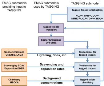
NMHC, which include all chemically active nitrogen com-pounds (15) and hydrocarbons (42) (see the Supplement for more details). All together, the tagging scheme consists of 7 species times 10 emission sectors, thus 70 tagged tracers. For each tracer initialisation, transport (except for OH and HO2), emissions, dry and wet deposition, and chemical

con-version has to be deduced from the base model (Fig. 1). The tagging scheme utilises the EMAC submodels, e.g. for tracer transport, for emissions computed online during the simula-tion, and for emissions prescribed by inventories (Table 1; for details see the Supplement), such as industry, road traf-fic, etc. (Fig. 1, middle column). It further obtains informa-tion on online emissions (lightning, soils), dry and wet depo-sition, background tracers and reaction rates (left column). This information is processed in tagging core routines (right column).

Here, we concentrate on the TAGGING submodel (Fig. 1, right column). For the initialisation of the tagged tracers two

options are available. First, the variables can be initialised from files, or second the tagged tracers can be initialised ac-cording to their key characteristics. In this case, the tagged stratospheric ozone is initialised by the ozone field above the tropopause and all other tagged ozone fields are zero above the tropopause and vice versa. Below the tropopause, all but the tagged stratospheric ozone tracer, obtain one-ninth of the tropospheric ozone concentration.

At each time step during the simulation, the online emis-sions (soil emisemis-sions) are added to the respectively tagged tracer (Table 2). The emission rate is obtained by recording the concentration of NOxbefore and after the calculation of

online emissions. The tagged lighting NOytracer obtains the

sim-Tagged Tracer Initialisation

NO_ytag_{, PAN}tag_{, CO}tag

NMHCtag_{, O}

3tag, OHtag, HO2tag

Tagged tracer chemistry Scavenging SCAV

Deposition DDEP

Tagged Tracer Transport

Online Emissions ONEMIS, LNOX

Tendencies for tagged tracers Sector Emissions

OFFEMIS

Chemistry MECCA

Tendencies for tagged tracers

T

ime loop

Lightning, Soils, etc.

Scavenging and deposition rates

Background concentrations and reaction rates

TAGGING submodel EMAC submodels

used by TAGGING EMAC submodels

providing input to TAGGING

Figure 1.Sketch of the tagging algorithm.

ple manner, by the difference in the respective concentrations before and after dry and wet deposition is calculated. This tendency of the concentration is provided to the tagging sub-model and distributed among the tagged species according to their relative contribution to the total concentration.

3.3 TAGGING chemistry

The core of the tagging submodel is the distribution of the chemical tendencies to the tagged tracers as introduced in Sect. 2. Therefore, the individual production and loss terms have to be determined adequately to calculate concentration changes via Eq. (7). Here, we consider effective ozone pro-duction and loss terms according to Crutzen and Schmaizl (1983). This implies that a family is considered for ozone (see Supplement for more details), which includes all fast exchanges between ozone and other chemical species. The ozone production basically requires splitting up an oxygen molecule. For the identification of ozone production and loss reactions, we apply the tool ProdLoss(see Supplement for more detailed information), which identifies the effective production and loss reactions for a family in the selected chemical mechanism. This family for effective ozone is here-after referred to as ozone for simplicity. This results in two ozone production terms, which are applied to any tagged ozone field with the exception of stratospheric ozone. This is Reaction (R1) and the combination of reactions of the type

(see Supplement for more detailed information)

NO+RO2−→NO2+RO (R2)

with reaction rate PR2. The production and loss terms of

these tagged ozone fields are then

PO3tag=

1 2PR1

NOtagy

NOy

+HO2

tag

HO2

!

(13)

+1 2PR2

NOtagy

NOy

+NMHC

tag

NMHC

!

,

DO3tag=

1 2PR3

_OHtag

OH +

O3tag

O3

(14)

+1 2PR4

_HO

2tag

HO2

+O3

tag

O3

+1 2PR5

NOtagy

NOy

+O3

tag

O3

!

+1 2PR6

_NMHCtag

NMHC +

O3tag

O3

+PR7

O3tag

O3

,

with “tag” denoting one of the 10 source tags and with the reaction ratesPR3,PR4,PR5,PR6,PR7referring to the

NMHC NO_y

O₃

CO PAN

OH HO₂

CH₄

CO₂ N₂O

Figure 2.Sketch of the chemistry of tagged species (blue) and key relations to other species (orange). Note that stratospheric ozone is not included here. For HOxchemistry see also Fig. 3.

OH+O3−→HO2+O2 (R3)

HO2+O3−→OH+2 O2 (R4)

Effective ozone loss via NOy (R5)

RO2+O3−→RO+2 O2 (R6)

OH+O3−→HO2+O2 (R7)

The tagged species NOy, CO, NMHC, and PAN are treated

similarly and will be discussed here only briefly, while more detailed information is provided in the supplement. Fig-ure 2 sketches the principal relations between the tagged species. Methane (not tagged) is depleted and the chemical products are then tagged as “NMHC from methane”. The species in the NMHC family are eventually transformed into CO and further into CO2. The decomposition of N2O (not

tagged) constitutes a source for “stratospheric NOy”.

Reac-tions between NOyand NMHCs form PAN (not included in

NOy). PAN is an important species, which can be transported

over long distances before it thermally decomposes (Roberts, 2007).

HOx chemistry (Fig. 3 and Table 3) and the calculation

of the individual contributions to the concentrations of OH and HO2is much more complex; hence, we discuss it here in

more detail. The main source of OH is the reaction of H2O

with O(1D). The chemical reactions between OH and HO2

involve species such as CO, CH4, NOy, and NMHC. Losses

of HOx are the formation of H2O2 and HNO3, which are

soluble and can be easily rained out.

Since the lifetime of both OH and HO2 is short, we

as-sume steady state for the contributions. We refer to the main HOx reactions, for which the production and loss rates are

calculated in and provided by the MECCA submodel (see also Table 2).

The steady-state assumption for the contributions to the OH and HO2 concentrations, i.e. OHtag and HOtag₂ , implies

that the individual production terms equal the individual loss terms:

P_OHtag=Ltag_OH, (15) P_HOtag

2 =L tag

HO2. (16)

Again the more complex part of the tagging chemistry is to derive the production and loss terms. Using the reactions in Table 3 and the approach from Grewe et al. (2010), we obtain for the production and loss of OHtag:

P_OHtag=P₁OHO3

tag

O3

+1 2P

OH 2

_HO

2tag

HO2

+O3

tag

O3

(17)

+1 2P

OH 3

NOtagy

NOy

+HO2

tag

HO2

!

,

Ltag_OH=LOH₁ 1 2

_OHtag

OH +

COtag CO

(18)

+LOH₂

_OHtag

OH

+LOH₃ 1 2

_OHtag

OH +

O3tag

O3

+LOH₄ 1 2

_OHtag

OH +

NMHCtag NMHC

+LOH₅ 1 2

_OHtag

OH +

HO2tag

HO2

+LOH₆ 1 2

OHtag

OH +

NOtagy

NOy

!

HO₂

NMHC OH

H2O

H₂O₂ O

+O D H₂O +O1_D

O3

O3 CH4

y NO_y NMHC

NMHC y

NO_y CO y

HNO₃ part of NOy

Figure 3.Atmospheric HOxchemistry used in the TAGGING scheme. Blue boxes indicate tagged species and families and orange circles

non-tagged species. Arrows indicate reactions.

Table 3.Reactions and reaction rates used for the calculation of OH and HO2contributions.

Reaction rate

Reaction OH HO2

Prod Loss Prod Loss

H2O+O(1D) −→ 2 OH 0.5P₁OH

HO2+O3 −→ OH+2 O2 P₂OH LHO₁ 2

NO+HO2 −→ NO2+OH P₃OH LHO₂ 2

OH+CO −→O2 HO₂+CO₂ LOH₁ PHO2 1

OH+CH4

O2

−→ NMHC+H2O LOH₂

OH+O3 −→ HO2+O2 LOH₃ P₂HO2

OH+NMHC −→O2 NMHC+H2O LOH4

OH+HO2 −→ H2O+O2 LOH5 L HO2 3

OH+NO2 −→ HNO3 LOH6

NMHC+NO −→ NMHC+HO2+NO2 P3HO2

NMHC+HO2 −→ NMHC+O2 LHO4 2

HO2+HO2 −→ H2O2+O2 LHO5 2

This set of equations includes the assumption that ex-changes within a family are fast enough to achieve equally distributed tags among family members. For example, con-cerningP₁OH, the contribution of one source to O(1D) equals that of O3, i.e.O(

1_D)tag O(1_D) =

O3tag O3 .

Similarly, we derive the individual production and loss terms for HO2:

P_HOtag 2 =P

HO2 1

1 2

_OHtag

OH +

COtag CO

(19)

+PHO2 2

1 2

_OHtag

OH +

O3tag

O3

+PHO2 3

1 2

NMHCtag

NMHC +

NOtagy

NOy

!

,

Ltag_HO 2 =L

HO2 1

1 2

_HO

2tag

HO2

+O3

tag

O3

(20)

+LHO2 2

1 2

HO2tag

HO2

+NO

tag y

NOy

+LHO2 3 1 2 _HO 2tag HO2 +OH tag OH

+LHO2 4 1 2 _HO 2tag HO2 +NMHC tag NMHC

+LHO2 5

HO2tag

HO2

.

Now the Eqs. (15) and (16) can be written as 0=Atag−LOHOH

tag

OH +P

OHHO2tag

HO2

, (21)

0=Btag+PHO2OH tag

OH −L

HO2HO2 tag

HO2

, (22)

with

Atag=P₁OHO3

tag O3 +1 2P OH 2

O3tag

O3 (23) +1 2P OH 3

NOtagy

NOy −1 2L OH 1 COtag CO − 1 2L OH 3

O3tag

O3 −1 2L OH 4 NMHCtag NMHC − 1 2L OH 6

NOtagy

NOy

,

Btag=1 2P HO2 1 COtag CO + 1 2P HO2 2

O3tag

O3 (24) +1 2P HO2 3 NMHCtag NMHC + 1 2P HO2 3

NOtagy

NOy

−1 2L

HO2 1

O3tag

O3

−1 2L

HO2 2

NOtagy

NOy −1 2L HO2 4 NMHCtag NMHC , POH=1

2

P₂OH+P₃OH−LOH₅ , (25) LOH=1

2

LOH₁ +2LOH₂ +LOH₃ (26) +LOH₄ +LOH₅ +LOH₆ ,

PHO2₌1 2

PHO2

1 +P

HO2 2

, (27)

LHO2₌1 2

LHO2

1 +L

HO2

2 +L

HO2 3

+LHO2 4 +2L

HO2 5

. (28)

The Eqs. (21) and (22) can easily be solved resulting in OHtag= A

tag_LHO2_+Btag_POH

LOH_LHO2−POH_PHO2OH, (29) HO2tag=

AtagPHO2_+Btag_LOH

LOH_LHO2−POH_PHO2HO2. (30) The quantity Atag (Btag) represents the contribution of chemical tracers (tagged and non-tagged, other than OH and

HO2) to the net OH production (net HO2production). The

termsLOH andPOH are primarily contributions to OH loss and production rates, which depend on the contribution to OH (OHtag) and HO2(HO2tag), respectively. Only the

reac-tion of OH with HO2forming water vapour and molecular

oxygen constitutes an exception, since the loss of OH is de-pendent on both OH and HO2(LOH₅ ). Therefore, it also

con-tributes toPOH(see Eq. 25), the last term in Eq. (21), which depends on HO2. Note that in this case it does not lead to a

production but destruction of OH.

4 Present-day simulation and comparison to other studies

In this section, we present results of a present-day simula-tion. An actual validation of the tagging method is not fea-sible, since only the full quantities can be measured, e.g. the ozone concentration, but not the contribution from individ-ual sources. Therefore, we concentrate on a comparison to earlier studies. In the following sections we present the sim-ulation set-up and give a plausibility check for contributions to the HOxconcentration based on shipping and aviation,

fo-cussing on the ozone concentration. 4.1 Simulation set-ups

4.1.1 EMAC

To evaluate the TAGGING submodel, we conduct two dif-ferent simulations, one base simulation with all emissions and a second simulation where we reduced all road traffic emissions by five percent. The set-up follows the “Specified Dynamics Reference Simulation” for the Chemistry Climate Model Initiative, and is identical to the RC1SD-base10a set-up described and evaluated by Jöckel et al. (2016), however, extended by the TAGGING module, which we described above.

The simulation is performed with a spectral resolution of T42 and a vertical resolution of 90 levels (up to 0.01 hPa). For the anthropogenic emissions we use the MACCity emissions dataset with a resolution of 0.5◦described by Granier et al. (2011). The lightning emissions are calculated online using the parameterisation described by Grewe et al. (2001). Emis-sions of NO from soil and biogenic origin as well as biogenic isoprene (C5H8) are calculated online by the MESSy

Figure 4.Annual mean contributions [ %] of 10 emission sectors to the simulated ozone volume mixing ratios. The simulated ozone volume mixing ratio is shown in the lower right panel.

One important difference of our simulation to the RC1SD-base10a set-up is the use of the QCTM mode of EMAC (Deckert et al., 2011). This QCTM mode decouples the chemistry and the dynamics by using monthly climatologies (here derived from the RC1SD-base10a simulation) in the radiation code and for the heterogeneous stratospheric reac-tions. The application of the QCTM mode is important for overcoming the problem of a low signal to noise ratio in the case of a direct comparison of a base case simulation with one, with a small chemical perturbation, which would be present with a fully coupled system. The dynamical and chemical differences between the RC1SD-base10a and our base simulation are shown in the Supplement. The simu-lation covers the period 2004–2010 and is initialised from the RC1SD-base10a simulation. The first year was used as a spin-up period, resulting in an evaluation period from 2005 to 2010.

4.1.2 MECO(n)

The COSMO/MESSy simulation shown in Sect. 5.1 covers the European domain, including parts of the eastern Atlantic and North Africa, with a resolution of 0.44◦_{(≈50 km).} Sim-ulated is the period from July 2007 until December 2008, with the 6 months of 2007 used as spin-up phase. The driv-ing EMAC model is applied at a resolution of T42 with 31 horizontal levels and is relaxed towards ERA-Interim reanal-ysis as well. The same QCTM mode as described above is ap-plied for EMAC and COSMO/MESSy. Both model instances use the anthropogenic MACCity emissions, as well as online calculated soil/biogenic emissions as described above. The

simulation differs, however, from the EMAC simulation de-scribed above, by using the lightning parameterisation after Price and Rind (1992) to simulate the lightning NOx

emis-sions on the global scale. In COSMO/MESSy we use the same emissions as on the global scale by regridding the cor-responding emissions from EMAC. We have chosen this ap-proach to have emissions as comparable as possible in both model instances. More detailed information about this simu-lation, including an evaluation of chemical tracer concentra-tions, is provided by Mertens et al. (2016).

4.2 Contributions of emission sectors to NOy, CO,

NMHCs, and O3

The 6-year annual average contributions of the 10 emission sectors to the ozone concentration are shown in Fig. 4. We compare these results with an earlier model version, which only tags NOy and ozone (Grewe, 2007, Fig. 5b therein),

and to earlier similar studies by Lelieveld and Dentener (2000) and Emmons et al. (2012). This comparison aims at verifying that the implementation of the TAGGING mechanism is correct by comparing contribution patterns and magnitudes. We have to keep in mind that the approach is conceptually different from earlier studies and takes into account all ozone precursor emissions and not only NOy.

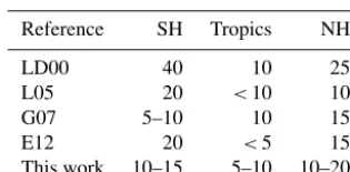
Table 4.Comparison of different studies with respect to the contri-bution (%) of stratospheric ozone to the tropospheric ozone concen-tration. Numbers are rough estimates only, as taken from published figures. Note that values for L05 are surface values only and per-centage values from E12 are estimated from mixing ratios; however, a mean value of 17 % is given therein. See text for more explana-tions. SH and NH are abbreviations for the Southern and Northern Hemispheres, respectively.

Reference SH Tropics NH

LD00 40 10 25 L05 20 <10 10 G07 5–10 10 15 E12 20 <5 15 This work 10–15 5–10 10–20

Grewe (2007), and Emmons et al. (2012) (hereafter denoted as LD00, L05, G07, and E12, respectively) estimated a 5– 40 % contribution from stratospheric ozone to tropospheric ozone in the Southern Hemisphere and mostly systematically lower values of 10–25 % in the Northern Hemisphere, while tropical values are below 10 % (Table 4). Our simulation also shows a minimum of the stratospheric ozone mixing ratios in the tropics and lower mixing ratios in the Southern Hemisphere compared to the Northern Hemisphere. The mixing ratios for January and July are very similar to those of Emmons et al. (2012, not shown).

Ozone formed from lightning NOx(Fig. 4) shows a

max-imum in the tropics and upper troposphere and larger con-tributions in the Southern Hemisphere than in the Northern Hemisphere, which is in agreement with G07 and LD00. The maximum contribution from lightning is around 25– 30 % and thus lower than G07 (40 %) and LD00 (50 %), be-cause here we regard the ozone production of all precursors, whereas in G07 and LD00 only NOx as a precursor is

con-sidered (see above).

Agreement between the studies LD00, G07, E12, and our work can also be found with respect to the contribution of anthropogenic emissions to tropospheric ozone. These emis-sions (here: anthropogenic non-traffic, road traffic, shipping, and aviation) predominantly contribute by 30–50 % in the Northern Hemisphere. The ozone contribution from biomass burning peaks in the lower tropical troposphere with val-ues of around 10–15 %, which compares well with G07 and LD00 (20 %). Around 15 % of the tropospheric ozone orig-inates from methane, which reacts with OH and contributes to NMHC compounds and eventually to CO and CO2.

Figure 5 shows the contribution of the individual emis-sion sectors to the tropospheric budgets of NOy, CO, NMHC,

PAN, and O3. Lightning and non-traffic anthropogenic

emis-sions show the largest contributions to NOy. The emitted

NOyfrom lightning and aviation remains much longer in the

atmosphere compared to a surface source, such as non-traffic anthropogenic NOy, since lightning and aviation emit mainly

in the upper troposphere. Aviation, shipping, and biomass burning have approximately the same contribution.

The different emission sectors have very different emis-sion characteristics. Some are only emitting NOy, such as

lightning, or NOy and NMHCs, such as most anthropogenic

sources. This is well reflected in the budgets (Fig. 5). Since NOyis required to form PAN, the decomposition of PAN also

produces NOy and NMHCs with the original tag, e.g. the

lightning tag. This is fully consistent with the chosen tag-ging approach and leads to minor contributions of non-CO and non-NMHC emitting emission sectors to the CO and NMHC budgets (lightning, stratosphere, aviation). For exam-ple, NOxemitted by road traffic may react with hydrocarbons

from, e.g., biogenic emissions to form PAN, which is then transported over longer distances. When decomposed after being transported over a long distance, the products obtain tags from both sources. Hence, hydrocarbons, which may not have been emitted by road traffic, obtain in this process a road traffic tag. The reasoning behind this is that only the PAN formation allowed for the long-range transport of ei-ther species and hence both emission sources have affected this. While this case is a wanted tagging effect, other situa-tions may lead to unwanted side effects or even unphysical effects (see discussion in Sect. 6 for more details). The for-mation of PAN and hence contributions to PAN (Fig. 5, sec-ond row) requires both NOy and NMHCs. None of the 10

emission sectors has a large contribution from both; hence, the contributions of each of the 10 sectors to PAN are almost equally distributed around 10 %. One exception is methane, which contributes largely to NMHC concentrations but not to NOy. In addition, the NMHCs from methane are

predom-inantly occurring in areas with low NOybackground, which

reduces the impact on PAN. The contribution to tropospheric ozone (Fig. 5, second row) reflects the distribution presented in Fig. 4, with major contributions from lightning, strato-sphere, anthropogenic non-traffic emissions, and methane. 4.3 Contribution of emission sectors to HOx

concentrations

In this section, we present the effects of a surface source (shipping) and a higher-altitude atmospheric source (avia-tion) on their contribution to the HOx concentrations. We

have chosen the Mediterranean Sea for shipping, since it in-cludes areas in the middle of the Sea on the one hand, as well as areas that are largely affected by other sources, e.g. in southern France (Marseilles) and Italy (harbour areas such as Genoa, Fig. 6), on the other hand.

We have identified four areas (A–D) with different chem-ical characteristics (Table 5, see also Fig. 6): highly polluted areas with high concentrations of NO2(A and B) and with a

large (some) impact from shipping in region A (B); a more remote area with some impact from shipping on NOxand O3

Figure 5.Contributions to the annual mean tropospheric budgets [Tg] of 10 emission sectors.(a–c)NOy, CO, and NMHCs;(d, e)PAN and

O3. Error bars indicate the interannual variability.

Table 5.Qualitative characterisation of four different regions (A–D) in the Mediterranean Sea. A: southern France; B: Strait of Gibraltar; C: central Mediterranean Sea; D: Tunesian coast. See Fig. 6 (top row) for the location of the regions. The signs “++”, “+”, “◦”, and “−” indicate a qualitative estimate of the respective characteristics, “very strong/very large”, “strong/large”, “moderate”, “negative”.

A B C D

Region has polluted background ++ + ◦ ◦

Region is impacted by shipping NOx ++ + + ++

Region is impacted by shipping ozone + + + ++

Shipping emissions are converting HO₂into OH via NO+HO₂−→OH + NO₂ ++ ++ + +

Shipping ozone produces OH via O₃−→O(1D)−→H2OOH + + + ++

Contribution of shipping emissions to OH − + ++ +

Contribution of shipping emissions to HO2 − − ◦ −

Large NOx concentrations in the background (A and B)

impact the chemistry and net production efficiencies; i.e. the ozone enhancement per NOx is decreasing with increasing

NOx concentrations (e.g. Dahlmann et al., 2011). The

Re-action (R1), which transforms HO2into OH, in principle

in-creases (dein-creases) the OH (HO2) concentration in the region

where large amounts of shipping NOx is present. However,

this reaction only dominates the OH to HO2ratio if enough

ozone is available for the HOx production. In region A, the

very low ozone concentration due to ozone titration by NOx

limits the availability of OH and the contribution of shipping NOx to OH is even negative. Region B is less polluted than

region A and has lower values of shipping NOx and

there-fore Reaction (R1) dominates the OH and HO2

contribu-tions from shipping, leading to positive contribucontribu-tions to OH and negative to HO2. The tagged shipping ozone is larger

reac-Figure 6. Absolute contribution of shipping to the simulated OH (a, c)and HO2(b, d)volume mixing ratios (in fmol mol−1)

for August 2007.(a, b)EMAC;(c, d)MECO(n). Regions A–D are characterised by different chemical situations. A: southern France; B: Strait of Gibraltar; C: central Mediterranean Sea; D: Tunesian coast; see text for more details.

tion of H2O with O(1D), where the O(1D) originates from

the tagged ozone (see also Table 3). The close coupling of OH with HO2 also enhances the tagged HO2 especially in

region D. These processes then lead to a complex picture. It shows negative contributions to OH in region A, mainly due to low ozone concentration limiting the OH availability, which is even more pronounced by shipping emissions. The shipping contribution to HO2in the polluted areas A and B

are negative mainly driven by the Reaction (R1). Large pos-itive contributions of shipping to OH and moderate negative contributions to HO2are found in region C, resulting from a

combination of effects from Reaction (R1) and the main OH production resulting from tagged shipping ozone, whereas in region D moderate positive contributions of shipping to OH and large negative contributions to HO2are found.

Over-all, the contributions from shipping emissions to the OH and HO2 concentrations show a complex picture, which results

from variations in both the background concentrations and shipping concentrations. The impact of an enhanced horizon-tal resolution is discussed for the same situation in Sect. 5.

Figure 7 shows annual mean contributions of aviation NOx

emissions to OH (left) and HO2(right). The air traffic

con-tribution to OH peaks at around 10–20 fmol mol−1 at the main flight altitude. At the surface, there are other secondary peaks, basically at the locations of the airports. Lee et al. (2010) summarised the work of Grewe et al. (2002) and Köh-ler et al. (2008) in their Fig. 10 and showed four atmospheric regions, which are affected differently by air traffic. In the first region (RNOy in their paper), which is mainly the air

traffic corridor, Reaction (R1) controls the chemical impact from air traffic emissions. This implies that air traffic largely contributes to OH and negatively contributes to RHO2 as

Figure 7.Annual mean absolute contribution [fmol mol−1] of avi-ation to the simulated OH(a)and HO2(b)volume mixing ratios.

The regions RO3, RNOy, and RHO2are characterised by distinct

different chemical response to aviation emissions as described by Grewe et al. (2002) (see text for further details).

shown in Fig. 7. The region north of RNOy is called RHO2

and the aviation impact is largely controlled by the reaction of O3with HO2(see Table 3). Hence, this reaction leads to

a reduction in HO2without affecting the OH concentration

in a similar manner. The region RO3is located in the lower

troposphere and away from the major flight corridor. Here, a significant contribution from air traffic to ozone is found, but not so much to NOy (not shown). The region is controlled

by an increase in ozone. Hence, it leads to a general increase in HOx via the reaction of H2O with O(1D) (see Table 3).

This comparison shows that the OH and HO2 contributions

from aviation, calculated here, are consistent with the chem-ical regimes identified in previous studies.

A more detailed view on this tagging mechanism is feasi-ble by applying it to a Lagrangian framework (Grewe et al., 2014). Within the EU-Project REACT4C (Reducing Emis-sions from Aviation by Changing Trajectories for the ben-efit of Climate), the HOx tagging mechanism was

imple-mented in the same EMAC model version, including a La-grangian transport algorithm. Aviation-like pulse emissions of NOx were released at selected points in the atmosphere,

and trajectories with these emissions were tagged so that reactions with the background can be determined in detail. Note that aviation is not emitting CO and NMHCs in our simulation; hence, the equations look simplified in Grewe et al. (2014) as the values for COtag and NMHCtag are zero (see Sect. 3.3). Figure 8 shows the temporal development of several NOx-related species (top and middle) as well as

ozone production and loss terms (bottom) for a pulse emis-sion at 45◦W, 50◦N and 300 hPa. The NOxemission induces

net production of Otag₃ (see Eq. 10 in Grewe et al., 2014), mainly via Reaction (R1) and enhanced HOtagx as calculated

via Eqs. (29) and (30). NOxreacts with OH and forms HNO3,

which eventually leads to washout and a reduction of NOtagy

within a few weeks. When NOtagx is no longer available for

O3production, O tag

Figure 8.Temporal development of NOx-related species (a: NOx

(red), O3(blue), CH4(green),b: OH (blue), HO2(red)) and

pro-duction or loss terms (c: cumulative O₃loss (blue) and cumulative O3production (red)) induced by a pulse emission at 45◦W, 50◦N

and 300 hPa on 23 December 2000. The discrimination between the regimes RegNOxand RegO3refers to the NOxdominated (days 1–

15 after emission) and the O3-dominated regime (days 16–90 after

emission), respectively.

chemical regime, where enough NOxis available to produce

larger amounts of ozone with RegNOx and the following

regime as RegO3 (see also Fig. 8). Regarding the

destruc-tion of CHtag₄ , these two regimes are also characterising the two different depletion pathways. First, as long as sufficient NOtagx is available, CHtag₄ is reduced because of an increase of

OHtagvia reaction (R1) (NOx-driven CH4destruction).

Sec-ond, when NOtagx is removed, OHtagis mainly produced via

photolysis of Otag₃ and the subsequent ReactionP₁OH (H2O

+ O1D→2OH). The tagged OH and HO2 are far lower in

the RegO3regime compared to the RegNOxregime (Fig. 8,

middle); consequently, the gradient in the O3-driven CH4

de-struction is not as steep. However, due to the longer time pe-riod, it dominates the total amount of methane destruction in this case, which can be seen from a budget analysis for the chemical regimes RegNOx (blue bars) and RegO3 (red

bars) given in Fig. 9. Note that the trajectory is transported into polar night around day 5, which leads to a reduction of OH and HO2 and a reduction of the photochemical

activ-ity. This example shows a reasonable temporal behaviour of the tagged species and it further shows how combining the tagging methodology and a Lagrangian transport algorithm results in a powerful tool, facilitating a detailed analysis of particular processes.

5 Sensitivities

In this section, we investigate if our tagging scheme responds reasonably to changes in resolution (Sect. 5.1) and emissions (Sect. 5.2). In general, there are no strict verification tests other than checking for plausibility and stability.

5.1 Higher resolution: MECO(n)

By applying the MECO(n) system (Kerkweg and Jöckel, 2012a, b; Hofmann et al., 2012; Mertens et al., 2016), we have increased the horizontal resolution over Europe by roughly a factor of 5, from a resolution of roughly 200 km times 300 km in EMAC to 50 km times 50 km in the nested grid. Figure 10 shows the contributions of the individual emission sectors to the tropospheric ozone column as a mean over Europe for the coarse resolution (top) and the finer reso-lution (bottom). Clearly, the individual contributions are very similar in terms of mean values and the seasonal cycle. The finer-resolution simulation shows finer-resolved structures in the horizontal (not shown), which, however, do not largely affect the large-scale budgets.

As an example of the effects of finer resolution, we present OH and HO2contributions from shipping over the

0 1 2 3 4 5 6 7 8

NO

x

HO

x

O

3 CH_4-LossO3-ProdO3-Loss

Mean mass (change) of NO

x

[10

5 kg],

HO

x

[10

4 kg], CH

4

[10

6 kg], O

3

[10

7 kg]

RegNOx RegO3

Figure 9.Mean contributions to NOx-related species and

produc-tion or loss terms for the RegNOxregime (NOxdominated, blue)

and RegO3 regime (O3dominated, red), respectively. Values are

given as temporal means over the two time periods.

to the OH concentration in the area of shipping emissions (B–D) and a decrease in the contribution to OH and HO2

where background NOxis largely enhanced (region A).

The comparison of the coarser and finer resolution clearly shows that the tagging scheme is stable in its behaviour. Nat-urally, the finer resolution enables more detailed and finer-resolved chemical changes due to emissions to be quantified, but basic structures are reproduced in either resolution. This implies that, depending on the underlying research question, either model can be used.

5.2 Emission changes

We performed an additional global simulation with EMAC where we reduced the road traffic emissions by 5 %. The simulation set-up hence follows Hoor et al. (2009). This means that the chemical composition and the ozone produc-tivity is different from the base simulation, which leads to a roughly 2–3 % reduction in the tagged road traffic ozone (not shown). Generally, a reduction of surface NOx

emis-sions is increasing the ozone productivity (Emmons et al., 2012; Grewe et al., 2012) and consequently a 5 % reduction in emissions is expected to lead to significantly less than a 5 % reduction in road traffic ozone, which is consistent with our results. Figure 11 shows the relative change in tropo-spheric ozone induced by the road traffic emission reduc-tion of 5 %. The total ozone change of 0.08 % (black bar) is a consequence of the reduction of the contribution of road traffic to the tropospheric total ozone by 0.16 % and other compensating effects. In total, this leads to a factor of 2 dif-ference between the total ozone change and the road traffic ozone change. The compensating effects are resulting from larger net ozone production rates for the shipping emission sector and other anthropogenic non-traffic emission sectors. This leads to a larger contribution of the anthropogenic

non-Figure 10.Contributions (fraction) of individual emission sectors to the European tropospheric ozone concentration for a coarser-resolution simulation with EMAC(a)and a finer resolution with MECO(n)(b)for the year 2008.

traffic (dark blue bar) and the (other than road traffic) traf-fic emission sectors (green bar) to total ozone by 0.04 and 0.06 %, respectively. Other non-anthropogenic sectors (red bar) , i.e. natural emission, reduce this compensation.

The ratio of 2 between the reduction in total ozone and road traffic indicates that a calculation of the road traffic contribution to tropospheric ozone using the perturbation method, i.e. difference between two simulations with chang-ing emissions, underestimates this contribution by exactly this factor of 2. Other studies have shown slightly larger fac-tors, e.g. a factor of 3 for biomass burning NOx emissions

(Emmons et al., 2012) and a factor of 5 for road traffic NOx

emissions (Grewe et al., 2012). Here, a smaller factor can be expected, since emissions other than NOx and their

Figure 11.Changes in the global tropospheric ozone budget [%] resulting from a 5 % reduction in the road traffic emissions.

6 Options, limitations, and future perspectives

The primary goal for developing this TAGGING submodel is to diagnose the impact of many individual emission sectors on radiatively active species, such as ozone and methane (via OH as the main methane loss process), in multi-decadal sim-ulations of the atmospheric composition. While this repre-sents a major improvement in comparison to many available tagging mechanisms, it also has its limitations. Such a mech-anism needs to be fast enough and to have a limited mem-ory demand. It is a trade-off between complexity, accuracy, and even correctness. The approach presented in Sect. 2 is an accurate and self-consistent decomposition of concentra-tions with respect to processes considered. In order to limit the memory demand, we have mapped the complex chem-istry scheme to a family concept, which reduces the num-ber of required additional tracers to a minimum. Obviously, this mapping represents a loss in accuracy and in some cases unwanted and unphysical effects may occur. While the ef-fect of mixing of tags through PAN processing is to some extent wanted (see discussion in Sect. 4.3), this also causes some unwanted effects. For example, during the degradation of methane, hydrocarbons are produced, which are classi-fied as the NMHC family. In reality, they are not contribut-ing to PAN formation, whereas in the taggcontribut-ing scheme, they are grouped in the NMHC category and thereby falsely con-tribute to PAN formation. Hence, the information on the type of hydrocarbons is lost in the family concept and represents an unphysical side effect. We might overcome these effects, at least to some extent by structuring the families in more detail. Such as different NMHC categories according to their number of C atoms. The coupling of families may represent

a major problem, since tags are mixed unwantedly between the families for fast exchange rates. Here, we concentrate on effective exchanges only. Hence, the introduction of PAN buffers, PAN-NHMC and PAN-NOy, together with a PAN

lifetime, may reduce this artefact. NOy from one emission

source, which forms PAN, will be accounted first in a buffer, which will decompose totally back to the original NOy

emis-sion source. Only, for long lifetimes of the formed PAN, a mixing of tags could be allowed.

We presented for the first time a HOxtagging mechanism,

which provides reasonable information on how individual emission sources contribute to OH concentrations. Here, we also have mapped the HOx chemistry to a reduced HOx

scheme. This leads to inaccuracies in the OH contributions, which are normally less than 10–20 %. First results show that an accuracy of less than 1 % can be achieved if the complete mechanism is taken into account (Rieger et al., 2017), which will be presented in a forthcoming paper. However, the re-spective changes on NOyand ozone are marginal.

7 Conclusions

We present a submodel for the Earth-System Model EMAC, which diagnoses online the contributions of individual source categories (mainly emission sectors) to the concentrations of various trace species. For the first time, we take into ac-count the competition of nitrogen oxides, carbon monoxide and non-methane hydrocarbons for the production and de-struction of ozone. We concentrated on 10 source categories and 7 species and families, which are tagged. As a result, we introduced 70 new tracers. The physical and chemical tendencies for these tracers are obtained from other sub-models of EMAC, such as chemistry (MECCA), scaveng-ing (SCAV), etc. The taggscaveng-ing mechanism is distributscaveng-ing the calculated physical and chemical tendencies into the tagged tracer fields. Therefore, the computing time increase by the TAGGING submodel is small, around 10 %.

We performed a present-day simulation and showed that the TAGGING submodel provides contributions of individ-ual emission sectors to the concentration of ozone, which roughly agree with previous estimates. A detailed analysis of the calculated contribution of aviation and shipping to OH and HO2 shows reasonable results in different

chemi-cal regimes. Changes in the model’s resolution show a sta-ble performance of the TAGGING submodel. Changes in the strength of road traffic emissions yield a decrease in ozone, which is partly compensated for by an increase in ozone from other source categories, since the ozone production efficiency increases, which is in agreement with earlier findings (Grewe et al., 2012; Emmons et al., 2012).

lin-earisation is required, and (4) the scheme is applicable for long-term simulations, e.g. over a century. On the other hand, the disadvantage is that (1) the family concept is not flexi-ble and fixed in this specific way, and consequently (2) any change in the set of chemical species requires an adaptation of the TAGGING scheme, and (3) due to memory limitations, a restriction to the main chemical species and families is re-quired.

To summarise, the TAGGING submodel provides a pow-erful tool to identify the contribution of individual emission sectors to main atmospheric constituents at every grid point and time step of the simulation and can be further used to derive, for instance, radiative forcings or contribution to air quality information for individual emission sectors.

Code availability. The Modular Earth Submodel System (MESSy) is continuously further developed and applied by a consortium of institutions. The usage of MESSy and access to the source code is licensed to all affiliates of institutions, which are members of the MESSy Consortium. Institutions can become a member of the MESSy Consortium by signing the MESSy Memorandum of Un-derstanding. More information can be found on the MESSy Con-sortium Website (http://www.messy-interface.org).

The Supplement related to this article is available online at https://doi.org/10.5194/gmd-10-2615-2017-supplement.

Competing interests. The authors declare that they have no conflict of interest.

Acknowledgements. This study has been conducted in the frame-work of the DLR projects VEU, VEU2 and WeCare. We gratefully acknowledge the computational resources provided by the Leibniz Supercomputing Centre (LRZ) in Garching and the German Climate Computing Centre (DKRZ) in Hamburg. We are thankful to Roland Eichinger, DLR, for a detailed internal review.

The article processing charges for this open-access publication were covered by a Research

Centre of the Helmholtz Association.

Edited by: Fiona O’Connor

Reviewed by: two anonymous referees

References

Butler, T. M., Lawrence, M. G., Taraborrelli, D., and Lelieveld, J.: Multi-day ozone production potential of volatile organic com-pounds calculated with a tagging approach, Atmos. Environm. 45, 4082–4090, https://doi.org/10.1016/j.atmosenv.2011.03.040, 2012.

Crutzen, P. J. and Schmaizl, U.: Chemical budgets of the strato-sphere, Planer. Space Sci. 31, 1009–1032, 1983.

Dahlmann, K., Grewe, V., Ponater, M., and Matthes, S.: Quantify-ing The Contributions Of Individual NOxSources To The Trend

In Ozone Radiative Forcing, Atmos. Environm. 45, 2860–2868, https://doi.org/10.1016/j.atmosenv.2011.02.071, 2011.

Deckert, R., Jöckel, P., Grewe, V., Gottschaldt, K.-D., and Hoor, P.: A quasi chemistry-transport model mode for EMAC, Geosci. Model Dev., 4, 195–206, https://doi.org/10.5194/gmd-4-195-2011, 2011

Dee, D. P., Uppala, S. M., Simmons, A. J., Berrisford, P., Poli, P., Kobayashi, S., Andrae, U., Balmaseda, M. A., Balsamo, G., Bauer, P., Bechtold, P., Beljaars, A. C. M., van de Berg, I., Biblot, J., Bormann, N., Delsol, C., Dragani, R., Fuentes, M., Greer, A. J., Haimberger, L., Healy, S. B., Hersbach, H., Holm, E. V., Isak-sen, L., Kallberg, P., Kohler, M., Matricardi, M., McNally, A. P., Mong-Sanz, B. M., Morcette, J.-J., Park, B.-K., Peubey, C., de Rosnay, P., Tavolato, C., Thepaut, J. N., and Vitart, F.: The ERA-Interim reanalysis: Configuration and performance of the data assimilation system, Q. J. Roy. Meteorol. Soc., 137, 553–597, 2011.

Dunker, A. M., Yarwood, G., Ortmann, J. P., and Wilson, G. M.: Comparison of Source Apportionment and Source Sensitivity of Ozone in a Three-Dimensional Air Quality Model, Environ. Sci. Tech. 36, 2953–2964, https://doi.org/10.1021/es011418f, 2002. Emmons, L. K., Hess, P. G., Lamarque, J.-F., and Pfister, G.

G.: Tagged ozone mechanism for MOZART-4, CAM-chem and other chemical transport models, Geosci. Model Dev., 5, 1531– 1542, https://doi.org/10.5194/gmd-5-1531-2012, 2012.

Granier, C., Bessagnet, B., Bond, T., D’Angiola, A., van der Gon, H. D., Frost, G., Heil, A., Kaiser, J., Kinne, S., Klimont, Z., Kloster, S., Lamarque, J.-F., Liousse, C., Masui, T., Meleux, F., Mieville, A., Ohara, T., Raut, J.-C., Riahi, K., Schultz, M., Smith, S., Thompson, A., Aardenne, J., Werf, G., and Vuuren, D.: Evolution of anthropogenic and biomass burning emissions of air pollu-tants at global and regional scales during the 1980–2010 period, Clim. Change, 109, 163–190, https://doi.org/10.1007/s10584-011-0154-1, 2011.

Grewe, V.: Technical Note: A diagnostic for ozone contribu-tions of various NOx emissions in multi-decadal

chemistry-climate model simulations, Atmos. Chem. Phys., 4, 729–736, https://doi.org/10.5194/acp-4-729-2004, 2004

Grewe, V.: Impact of climate variability on tropospheric ozone, Sci. Total Environ., 374, 167–81, 2007.

Grewe, V.: A new method to diagnose the contribution of anthro-pogenic activities to temperature: temperature tagging, Geosci. Model Dev., 6, 417–427, https://doi.org/10.5194/gmd-6-417-2013, 2013a.

Grewe, V.: A generalized tagging method, Geosci. Model Dev., 6, 247–253, https://doi.org/10.5194/gmd-6-247-2013, 2013b. Grewe, V., Brunner, D., Dameris, M., Grenfell, J.L., Hein, R.,

Shin-dell, D., and Staehelin, J., Origin and variability of upper tro-pospheric nitrogen oxides and ozone at northern mid-latitudes, Atmos. Environ. 35, 3421–3433, 2001.

Grewe, V., Dameris, M., Fichter, C., and Lee, D.: Impact of aircraft NOx emissions, Part 2: Effects of lowering the flight altitude,

Meteorol. Z., 3, 197–205, 2002.