R E S E A R C H A R T I C L E
Open Access
A comparison of genomic profiles of
complex diseases under different models
Víctor Potenciano
1, María Mar Abad-Grau
1*, Antonio Alcina
2and Fuencisla Matesanz
2Abstract
Background: Various approaches are being used to predict individual risk to polygenic diseases from data provided by genome-wide association studies. As there are substantial differences between the diseases investigated, the data sets used and the way they are tested, it is difficult to assess which models are more suitable for this task.
Results: We compared different approaches for seven complex diseases provided by the Wellcome Trust Case Control Consortium (WTCCC) under a within-study validation approach. Risk models were inferred using a variety of learning machines and assumptions about the underlying genetic model, including a haplotype-based approach with different haplotype lengths and different thresholds in association levels to choose loci as part of the predictive model. In accordance with previous work, our results generally showed low accuracy considering disease heritability and population prevalence. However, the boosting algorithm returned a predictive area under the ROC curve (AUC) of 0.8805 for Type 1 diabetes (T1D) and 0.8087 for rheumatoid arthritis, both clearly over the AUC obtained by other approaches and over 0.75, which is the minimum required for a disease to be successfully tested on a sample at risk, which means that boosting is a promising approach. Its good performance seems to be related to its robustness to redundant data, as in the case of genome-wide data sets due to linkage disequilibrium.
Conclusions: In view of our results, the boosting approach may be suitable for modeling individual predisposition to Type 1 diabetes and rheumatoid arthritis based on genome-wide data and should be considered for more in-depth research.
Background
Genome-wide association studies are being used to build multimarker predictive models of individual susceptibil-ity to complex diseases, referred to as genomic profiling or genomic predictors of genetic risk. The most common approach is to use simple logistic regression on a genome-wide genetic risk score (GRS) counting down the number of risk variants an individual has [1–5] or on a weighted GRS (wGRS) [1–8] that uses the log odds ratio (OR) for the disease associated with each position to weigh the effect of each genetic variant on the disease outcome. Logistic regression with wGRS is equivalent to the sim-pler Bayesian network defined for classification, the naïve Bayes classifier, which has also been used for this purpose [9, 10]. Multiple logistic regression is also an option in genome-wide data [11, 12] if some strong restriction to the
*Correspondence: [email protected]
1Departamento de Lenguajes y Sistemas Informáticos, ETSIIT, c/ Periodista Daniel Saucedo Aranda s/n Universidad de Granada, Granada 18071, Spain Full list of author information is available at the end of the article
number of input variables considered is imposed for them to be computationally feasible.
The most common statistic used to measure the quality of a risk predictor is the C-statistic or the area under the receiver operating characteristic (ROC) curve (AUCROC or AUC), which measures how well it can distinguish prediction rates between the two diagnostic groups (in genomic profiling, disease risk prediction between dis-eased and normal individuals).
In polygenic diseases, successful assessment of risk pre-diction is not only a matter of the accuracy of method used but a question of genetic epidemiology (i.e. disease prevalence and heritability). Disease prevalence,K, is the proportion of diseased individuals in a population [13]. Heritability may be measured byλs, the sibling risk ratio or ratio of the prevalence of disease in siblings of affected individuals compared to the prevalence in the population K[13]. A highly polygenic disease has a mild genetic com-ponent (i.e. modest heritability and high prevalence). The
more polygenic a disease, the greater the number of asso-ciated variants and the smaller their effect on the disease. Given a value reported by a statistic of fitness, there is no way of knowing which part represents model fitness to the true genetic risk of individuals and which part represents disease epidemiology (i.e. how well the true genetic risk predicts disease status) [13]. In order to help differentiate these two components of the AUC statistic, theAUCmax measure should also be used. TheAUCmaxmeasures the genetic component (i.e. the maximum AUC possible for there to be the perfect predictor of disease risk) ([13]) so that it will be lower in highly polygenic diseases.
At times, statistics of fitness such as the AUC are not even reported for genomic predictors possibly because they are much lower than risk predictors built on pheno-type and environmental data collected from medical tests or questionnaires. This is the case of studies on depres-sion and anxiety [6]. In other cases, there is no or only a modest AUC improvement (of no more than 0.01) when a GRS is added to traditional risk factors, such as in the case of coronary artery disease (CAD) [5, 14], myocardial infarction in Hispanics [15] or atherosclerosis [16]. Even if there were an improvement of more than 0.01, this is much lower than it should be considering the genetic epi-demiology of the disease. This is the case of predictors for rheumatoid arthritis (RA) [17] and lung cancer [4]. By way of example, in the predictor of lung cancer, the pre-dictive AUC in a within-study validation approach using bootstrapping was 0.639 [4] while the AUCmax is 0.98, AUChalf (the AUC when only half the genomic variants are included) is 0.89 andAUCquar (only a quarter of the variants are included) is 0.80 for lung cancer [13].
Most of these studies showed negative results as their predictive values were too low for them to be considered clinically useful when applied to a sample at risk [18]. Moreover, for highly polygenic diseases, their AUC scores were much lower than they should have been according to disease heritability and prevalence [13].
Additional file 1: Table S1 shows 6 of the 7 diseases from the WTCCC used in this study ordered according to their genetic component or polygenic level in terms of theAUCmax(column four). Prevalence and heritability are also shown (columns 3 and 4, respectively). These results were taken from Wray et al. 2010 [13]. The results shown for irritable bowel disease (IBD) were actually reported very similar disease, Crohn’s disease. There is no infor-mation about prevalence and heritability in hypertension (HT).
One interesting exception for a highly polygenic disease (AUCmax = 0.92) is a predictor of age-related macular degeneration built as a wGRS from only 13 risk variants, reporting an AUC of 0.84 [19], while theAUCmax,AUChalf andAUCquar[13] are 0.92, 0.81 and 0.72, respectively. An independent validation data set was not used to confirm
this result in order to detect possible AUC over-estimation because of a biased data set, possibly due to cases sharing other traits such as a higher average body mass index than the controls. However, even if the data set were not biased and the AUC had been correctly estimated, it should be noted that only individuals with both eyes affected and at least one having a severe form of age-related macular degeneration were selected. The reference max, half and quart AUCs do not therefore hold but much higher val-ues may be obtained since the authors are considering a very aggressive type of age-related macular degeneration which may have a much higher heritability [20].
The opposite of a highly polygenic disease is one that is not very polygenic (shown in the last rows of Table 1), i.e. those with high heritability and low prevalence and therefore a highAUCmax [13]. Extreme examples of not very polygenic diseases are Type 1 diabetes, Crohn’s dis-ease and systemic lupus erythematosus, which all have AUCmax=1 [13]. Two issues in highly polygenic diseases, which have been identified as responsible either for the negative results or for over-estimating classifier perfor-mance [2, 3, 7, 15, 21–23], have been successfully handled in not very polygenic diseases.
The first issue relates to the use of prior information from GWAS with low power. Low accuracy was there-fore due to the limited number of susceptibility variants detected in previous studies [18], which were used as the only input variables to build the predictor. In order to solve this, many of them selected markers on the basis of predefined thresholds for thep-values associated with the disease in the training data set [2, 18]. This approach was expected to perform better and in fact it did for the unpolygenic disease Type 1 diabetes when the algorithms used to model the classifier were robust to redundant or noisy variables, since variables associated with the disease in a real yet low-level way might well be detected through this approach [18].
Table 1Model learned from the T1D data set. Model learned from the T1D data set using 1-e5 as thep-value threshold, the holdout approach, AdaBoostM1 as the learning algorithm with default configuration (decision stump as the weak learning algorithm and 10 iterations)
Chr Chr SNP Allele Allele Weight Genotypes Weight Genotypes
# Pos 1 2 rule 1 rule 1 rule 2 rule 2
1 77051324 SNP_A−1827111 A C 0.0801 {0, missing}
6 32444658 SNP_A−1934589 A G 0.2326 {0}
6 30135583 SNP_A−2111335 A G 0.2171 {0} 0.0543 {1}
6 31395153 SNP_A−2079423 C T 0.1525 {0,1}
6 30390814 SNP_A−2222387 A G 0.0672 {0,1}
6 31112694 SNP_A−4293786 C T 0.0517 {0,1}
19 39266932 SNP_A−4281637 A G 0.0904 {0,1}
Weights and genotypes values are referred to class 1, i.e. absence of disease. Chromosome positions correspond to assembly NCBI dbSNP GRCh38.p2
power of the study is low [24, 26]; and the third is to use other approaches which are more robust to redundant or noisy variables. The third alternative was somehow suc-cessful in a study conducted on Type 1 diabetes [18], as the AUC score in a within-study 5-fold cross-validation approach was 0.89. It should be noted that theAUCmax is 1,AUChalf is 0.93 andAUCquar is 0.84 for Type 1 dia-betes [13]. However, looking in depth at the way the work was conducted, it seems that they added a set of 45 known susceptibility markers for Type 1 diabetes to the predic-tion model and some of these markers were obtained by a pooling study using, among other things, the analyzed data set [27].
As previously mentioned, however, the current chal-lenge is to handle these issues in highly polygenic diseases. To the best of our knowledge, no sound genetic predic-tor with a predictive AUC near its expected value [13] in terms of the genetic disease epidemiology has yet been built for any highly polygenic disease.
One possible reason for these negative results relates to the use of too simplistic models that assume marker inde-pendence and which may be unable to control redundant or noisy variables. However, there has been no success when predictive models capable of handling marker inter-actions and variable redundancy have been built under different approaches as a way to improve the predictive capacity, such as support vector machines [18], decision trees, random forests and boosting algorithms [28]. By way of example, in multiple sclerosis (MS), the AUC did not increase when other algorithms building more com-plex models (e.g. the Tree Augmented naïve Bayes classi-fier or a random forest) were used instead of a naïve Bayes classifier [28].
To the best of our knowledge, no systematic study with the purpose of building predictors for complex diseases of different epidemiological patterns, under different statis-tical approaches which is able to represent marker inter-actions and/or handle redundant or noisy variables, has
yet been conducted. We are therefore unable to conclude whether more complex models are the key to turning the current discouraging results into positive ones.
Perhaps, the lack of positive results may be due to a bias in most of the models used so far to represent marker dependencies and the implicit assumptions they rely on should be explored. Consequently, most of the attempts tried so far ignored chromosomal information. One result supporting this hypothesis was undertaken for Crohn’s disease [24] by a haplotype-based predictor. Although the predictive AUC was still too low (0.72) to be considered a positive result (AUCmax,AUChalf andAUCminare 1, 0.95 and 0.86 [13], respectively), it was much higher than when haplotype information was ignored (0.655). The authors only used haplotypes of 2-SNP length. There is still the question of whether the AUC would have improved if longer haplotypes had been used. As previously men-tioned [24], long haplotypes in case/control data sets may not be a solution as they are inferred with an important lack of accuracy. However, small haplotypes such as those of 3, 4 or 5 SNP length were not tried either. The authors also noted that signal dilution is less severe in shorter hap-lotypes. However, certain procedures for avoiding signal dilution could be used [29].
With this purpose, we performed a comparative study of the predictive capacity of disease predictors built with learning algorithms under different statistical approaches for 7 different diseases with different levels of the genetic component (Table 1). We also used a haplotype-based approach with haplotypes of different lengths from 1 to 5 in order to understand the importance of using chromo-somal information.
Results
Genotype-based predictors
We applied the common genotype-based model on a wide variety of approaches ranging from the most sim-ple (e.g. simsim-ple logistic regressions built on weighted or unweighted genetic risk scores and naïve Bayes classifiers) to the more complex (e.g. support vector machines or random forests which are capable of modeling variable interaction and handling redundant or noisy variables). Although multiple logistic regression may also deal with redundant or noisy variables, given their highly consuming processes of model building, they are not time-feasible without imposing some limit on the number of input variables used in genome-wide datasets. As the next subsection outlines, this limitation may lead to worse pre-dictive models than machine-learning approaches which are able to handle hundreds of thousands of variables more efficiently.
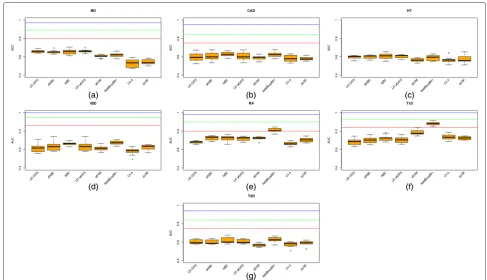
Figure 1(a)–(g) show the AUC values for each of the 7 diseases used in this work. Each figure compares results using logistic regression on a GRS (LR GRS), logistic regression on a wGRS (LR wGRS), a naïve Bayes clas-sifier (NBC), an allelic naïve Bayes clasclas-sifier assuming the two allelic variables for each position are identically distributed and conditionally independent given the trait (aNBC) [31], a sigmoid-based support vector machine (sSVM), a boosting algorithm (AdaBoostM1), a decision tree learning algorithm (c4.5) and 20 a random for-est learning algorithm (20RF) (see Methods for a short description of sSVM, AdaBoostM1, C4.5 and 20RF).
With the exception of the hypertension plot for which we do not have the necessary data, all the plots show three horizontal lines with the expected AUC when all, half and a quarter, respectively, of the known genetic variance is explained by the variants included in the model, as pub-lished in [13]. It can be observed how the predictive AUC reached at least AUCquar for only two diseases (Type 1 diabetes and rheumatoid arthritis). The genetic compo-nent of these two diseases is high (AUCmaxis 1 and 0.98, respectively). However, the predictive AUC for irritable bowel disease, an extremely unpolygenic disease, which every algorithm obtained, is far lower thanAUCquar.
Focusing on the algorithm used, the winning algorithm for these two diseases is AdaBoostM1. AdaBoostM1 is actually the only algorithm that outperformsAUCquar in
two diseases: rheumatoid arthritis (the mean predictive AUC is 0.8087, far higher than 0.7248, the second highest predictive AUC, obtained by allelic NBC) and Type 1 dia-betes (the mean predictive AUC is 0.8805, far higher than 0.7849, the second highest predictive AUC, obtained by sSVM, another complex algorithm).
Therefore, for Type 1 diabetes, two algorithms (AdaBoostM1 and sSVM) obtained a predictive AUC of over 0.75, the threshold required for a risk classifier to be clinically useful when applied to a sample at increased risk [32]. However, AUC superiority of AdaBoostM1 was statistically significant (α level 0.01,p-value was 0.00256 in a Wilcoxon Signed-Rank computed on the 10 folds). For rheumatoid arthritis only AdaBoostM1 managed to build a clinically useful disease predictor. For every other disease, no algorithm would be clinically useful for a sam-ple at risk, even less so for application as a diagnostic test in the general population. It should be noted that in order for it to be useful for the general population, the predictive AUC has been estimated at over 0.99 [32]. The negative results obtained by LR GRS and LR wGRS concur with previously published ones using the same data sets [2].
Fig. 1Boxplots for predictive AUC of genotype models. Boxplots for the predictive AUC obtained for each fold in the 10-fold cross-validation (cv) approach used to learn genotype models from data under different algorithms:aResults for bipolar disorder (BD),bcoronary artery disease (CAD), chypertension (HT),dirritable bowel disease (IBD),erheumatoid arthritis (RA),fType 1 diabetes (T1D) andgType 2 diabetes (T2D). For each plot (with the exception of hypertension where data was unknown), three horizontal lines are also plotted corresponding toAUCquar(red line),AUChalf (green line) andAUCmax(blue line) [13]
individual with the following genotypes 120?021 (where ? means a missing genotype), 0 no copies of allele 1 (i.e. homozygous for allele 2), 1 heterozygous and 2 homozy-gous for allele 1, will havep=0+0+0.2170542636+0+ 0+0+0.0904392765 = 0.3074935401 of being healthy or 1 − p = 0.6925064599 probability of having Type 1 diabetes, as the individual only has two genotypes for protection against the disease:SNPA−2111335 at chro-mosome 6 and SNPA−428163 at chromosome 19 (see columns 6 and 8 for genotype values associated with class 1), thereby increasing the probability of being healthy.
What is interesting from this approach is that this reduced model, which is learned from a training data set of only 1722 individuals, obtained a predictive AUC of 0.822 with only 7 SNPs, still higher than the second best result of 0.8112 obtained by 20RF (see Additional file 1: Table S2) under the same holdout approach. It should be noted that the classic models LR GRS and LR wGRS achieved much lower values: 0.7126 and 0.7294, respectively.
As mentioned previously, however, the more sophis-ticated model learning approaches (e.g. boosting algo-rithms, SVM or random forest classifiers) were only clinically useful when applied to a sample at risk in Type 1 diabetes and rheumatoid arthritis.
In order to study model reproducibility, we switched training and test data sets and ran AdaBoostM1 again under the same default configuration. The new model contains 9 different SNPs and is shown in Table 2.
In the two models, all SNPs at chromosome 6 belong to the MHC region (chromosome positions from 28510120 to 33480577 under assembly GRCh38.p2).
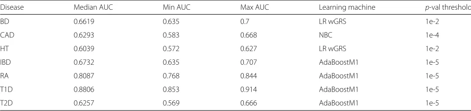
Table 3 shows the AUC results under the genotype-based approach with 10-fold cross validation (more detailed results are displayed in the Additional file 1: Tables S2 and S5 and other measures of fitness in the Additional file 1: Table S6–S8).
For comparative purposes with the haplotype-based approach that will be explained below, we have repeated the genotype-based model by using the same sampling approach used by the haplotype-based one: the holdout sampling. Otherwise, the AUC results for the haplotype-based models compared with the genotype-haplotype-based mod-els could be underestimated since only half the samples (holdout testing approach) were used as the training test while the original genotype-based models used 9/10 of the samples (10-fold cross validation testing approach).
Table 2Study of model reproducibility: model learned from the T1D data set by switching training and test data subsets. Model learned from the T1D data set, with the same configuration as the model in Table 5 but switching training and test data subsets
Chr Chr SNP Allele Allele Weight Genotypes Weight Genotypes
# Pos 1 2 rule 1 rule 1 rule 2 rule 2
6 32444658 SNP_A−1934589 A G 1.09 {0} 0.22 {1}
6 30135583 SNP_A−2111335 A G 0.74 {0}
6 32444815 SNP_A−4303523 A G 0.62 {0, 1}
6 30726039 SNP_A−2240847 A G 0.3 {0, 1, missing}
19 39266932 SNP_A−4281637 A G 0.41 {0,1}
6 31112694 SNP_A−4293786 C T 0.29 {0,1}
6 31277959 SNP_A−1863445 A G 0.31 {0,1}
6 31278044 SNP_A−1949560 A G 0.29 {0,1}
1 113630788 SNP_A−2235405 A G 0.2 {0}
Weights and genotypes values are referred to as class 1, i.e. absence of disease
validation. Detailed results can be found in Additional file 1: Tables S3 and S10 and other measures of fitness in Additional file 1: Tables S11–S13.
Variable selection and multiple logistic regression
We wanted to compare these AUC results with some state-of-the-art regression models, taking into account the fact that for them to be applied in genome-wide data sets we would need to impose some limit to the max-imum number of input variables so that they became computationally affordable.
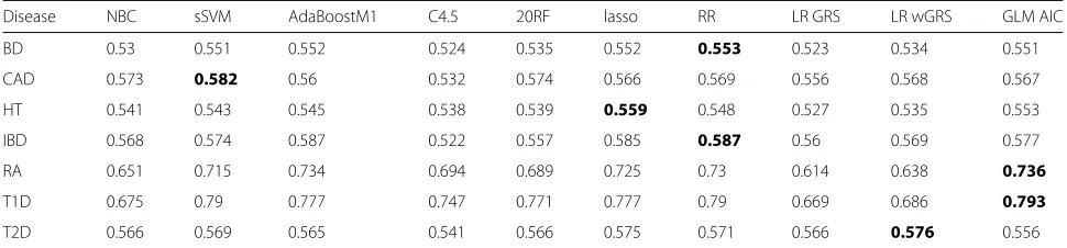
Table 4 shows the AUC under the holdout approach obtained by the different algorithms using only the top 100 SNPs (lowestp-value) selected from the training dataset to avoid cheating [11]. We used 100 variables because this was the number of SNPs that achieved the best results in Type 1 diabetes and Crohn’s disease in a similar study [11]. Several multiple logistic regression methods such as penalized regression methods (ridge regression –RR– [34] and the lasso [35]) and stepwise fitting of GLM with AIC to select variables (GLM AIC were used.
Column 5 of Table 5 shows the best AUC under the holdout approach when only the top 100 SNPs are used. The method that achieved this highest AUC is shown
in column 6. It can be seen how the AUC was always below that obtained when the number of variables was not limited (column 2).
A haplotype-based approach
In light of the discouraging results when using genotype-based risk predictors in most of the diseases analyzed, even when more sophisticated algorithms were tested, we tried to enhance the information provided to a learning machine to build the risk predictor by keeping as much chromosomal (allelic) association as possible. With this goal, in a second step we built several haplotype-based models as explained in Methods.
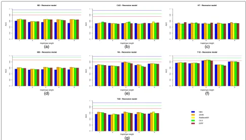
Figure 2(a)–(g) show bar plots with the AUC values cor-responding to the test data set for the 7 diseases and all of the different haplotype lengths used from 1 to 5 and all the learning machines built (i.e. naïve Bayes classifier (NBC), sSVM, AdaBoostM1, C4.5 and 20RF) under an additive genetic model.
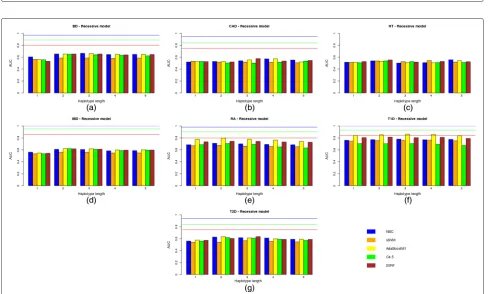
The same results but for a dominant and recessive genetic model are shown in Figs. 3(a)–(g) and 4(a)–(g), respectively.
Regarding the haplotype length, it is interesting to note that the approach based on haplotypes comprising only
Table 3Highest AUC obtained by the genotype-based approach under the 10-fold cross validation sampling model
Disease Median AUC Min AUC Max AUC Learning machine p-val threshold
BD 0.6619 0.635 0.7 LR wGRS 1e-2
CAD 0.6293 0.583 0.668 NBC 1e-4
HT 0.6039 0.572 0.627 LR wGRS 1e-2
IBD 0.6732 0.635 0.707 AdaBoostM1 1e-5
RA 0.8087 0.768 0.844 AdaBoostM1 1e-5
T1D 0.8806 0.853 0.914 AdaBoostM1 1e-5
Table 4AUC under the holdout approach and different genotype-based predictors learned using only the 100 top SNPs
Disease NBC sSVM AdaBoostM1 C4.5 20RF lasso RR LR GRS LR wGRS GLM AIC
BD 0.53 0.551 0.552 0.524 0.535 0.552 0.553 0.523 0.534 0.551
CAD 0.573 0.582 0.56 0.532 0.574 0.566 0.569 0.556 0.568 0.567
HT 0.541 0.543 0.545 0.538 0.539 0.559 0.548 0.527 0.535 0.553
IBD 0.568 0.574 0.587 0.522 0.557 0.585 0.587 0.56 0.569 0.577
RA 0.651 0.715 0.734 0.694 0.689 0.725 0.73 0.614 0.638 0.736
T1D 0.675 0.79 0.777 0.747 0.771 0.777 0.79 0.669 0.686 0.793
T2D 0.566 0.569 0.565 0.541 0.566 0.575 0.571 0.566 0.576 0.556
The highest AUC for each disease is shown in boldface
two SNP positions [24] has been improved by a more general approach in which different numbers of SNPs, i.e. haplotype lengths, were tested. Although the accu-racy of inferred haplotypes increased with the number of markers used, a modest number of SNPs of between 2 and 3 seem to obtain the best trade-off between haplo-type accuracy and model fitting. For HT, the best solution (AUC 0.5573) was obtained by all the genetic models used with NBC and haplotypes comprising 5 SNPs. How-ever, it should be noted that the AUC is too low and is outperformed by the genotype-based model. Therefore, haplotypes which are greater than 3 do not return better results. As already mentioned [24], this may be due to the decrease in accuracy of the reconstructed haplotypes.
Table 5 shows the best predictive AUC under the genotype-based approach (columns 2 and 5) and the haplotype-based approaches (column 7). More detailed results can be seen in Additional file 1: Table S4 and S15– S29 and other measures of fitness in Additional file 1: Tables S30–S74.
Although multiple logistic regression seems to outper-form modern classifiers such as sSVM or AdaBoost in most diseases under the same conditions, they are clearly
below the AUC achieved when all the SNPs were used. By comparing results with no variable filtering exceptp-value thresholds, and according to our results, AdaBoostM1 seemed to be the best among all the learning approaches used. It therefore outperformed all the others in five out of the seven diseases for both the genotype-based and haplotype-based models. Regarding the genetic model used, the additive approach outperformed or equaled all the others in five out of the seven diseases, although this result was not statistically significant (p-value is 0.4086 in a paired Student t-test on the null hypothesis of no superiority of the additive model over the recessive and dominant models).
The AUC results showed no absolute winner between the genotype and haplotype approaches (p-value was 0.8984 in a 2-tail Student t-test). The haplotype-based approach outperformed the genotype-based one in only 4 out of the 7 diseases analyzed, and the differences in AUC were low for most of these. The largest difference in AUC between the two approaches was reached in bipolar disor-der (BD) (0.6222 for the genotype-based approach versus 0.6873 for the haplotype-based approach). However, the AUC is still a long way from its expected value even when
Table 5Highest AUC obtained by the genotype and the haplotype-based approaches
Genotype-based, holdout approach Haplotype-based, holdout approach
p-value filtering Top 100 SNPs
Disease AUC Learning p-value AUC Learning AUC Learning Haplotype Threshold
machine threshold machine machine length p-value
BD 0.6222 LR wGRS 15e-2 0.553 RR 0.6873 AdaBoostM1-add. 3 1e-4
CAD 0.611 20RF 1e-5 0.582 sSVM 0.5761 20RF-rec. 3 1e-7
HT 0.5776 AdaBoostM1 15e-2 0.559 lasso 0.5573 NBC-all 5 1e-5
IBD 0.6136 AdaBoostM1 1e-5 0.587 RR 0.6213 AdaBoostM1-rec. 2 1e-5
RA 0.8152 AdaBoostM1 1e-5 0.736 GLM AIC 0.8024 AdaBoostM1-add. 2 1e-5
T1D 0.8615 AdaBoostM1 1e-5 0.793 GLM AIC 0.8682 AdaBoostM1-add. 3 1e-6
T2D 0.6134 AdaBoostM1 1e-3 0.576 LR wGRS 0.6372 AdaBoostM1-add. 2 1e-4
Fig. 2Predictive capacity of the haplotype-based approach under an additive genetic model. Predictive capacity of the haplotype-based approach under an additive genetic model: the AUC in the test data set is shown for different learning machines and the seven diseases of bipolar disorder (a), coronary artery disease (b), hypertension (c), irritable bowel disease (d), rheumatoid arthritis (e), Type 1 diabetes (f) and Type 2 diabetes (g)
Fig. 4Predictive capacity of the haplotype-based approach under a recessive genetic model. Predictive capacity of the haplotype-based approach under a recessive genetic model: the AUC in the test data set is shown for different learning machines and the seven diseases of bipolar disorder (a), coronary artery disease (b), hypertension (c), irritable bowel disease (d), rheumatoid arthritis (e), Type 1 diabetes (f) and Type 2 diabetes (g)
only a quarter of the known genetic variance is explained by the variants included in the model (AUCquart =0.80), meaning that the potential this approach may have for some diseases is still very limited in terms of practical use, such as medical profiling of highly polygenic diseases.
Comparing the three different genetic models used, there do not seem to be any significant differences between them. Summary Table 6 shows the highest AUC achieved by each genetic model for each disease, among all the predictive methods and haplotype lengths used.
Table 6Highest AUC obtained by the haplotype-based approach for all the genetic models used
Disease Additive Dominant Recessive
BD 0.6873 0.687 0.6649
CAD 0.5736 0.5733 0.5761
HT 0.5573 0.5573 0.5573
IBD 0.6196 0.6184 0.6213
RA 0.8024 0.7968 0.7971
T1D 0.8682 0.8609 0.8633
T2D 0.6372 0.6364 0.6355
The highest AUC of all haplotype lengths and predictive methods used obtained for each disease by the haplotype-based approach for additive, dominant and recessive genetic models
Values are very similar. For hypertension, the AUC is exactly the same for the three genetic models (0.5573).
Discussion
In light of our results, it seems that some of the new learning approaches strongly outperform the classic methods for them to be used for diagnosis purposes when used with a sample at risk in two of the seven diseases ana-lyzed: Type 1 diabetes and rheumatoid arthritis. This is the case of boosting methods, random forests algorithms and support vector machines in Type 1 diabetes and only boosting methods and random forests in rheuma-toid arthritis. Their ability to model variable interaction, however, seems not to be the reason for them to work, as AdaBoostM1 assumes variable independence in the same way as logistic regression or naïve Bayes classifier do. The reason may be their robustness to noisy or redundant variables [18] as they always include a method for vari-able selection (sSVM), pruning (20RF, C4.5) or weighting (AdaBoostM1).
The fact that Type 1 diabetes and rheumatoid arthri-tis are autoimmune diseases may indicate some common genetic cause. Additional file 1: Table S1 shows common SNPs between the winning configuration for both diseases (AdaBoostM1 as machine learning and p-value thresh-old of 1e− 5). All but four SNPs belong to the major histocompatibility complex (MHC).
In order to compare these common SNPs with those selected in other autoimmune diseases, we have also added results for multiple sclerosis (MS). With this goal, we used genetic data from the International Multiple Sclerosis Genetic Consortium (IMSGC) [36] comprising 931 family trios, and built models under the same algo-rithms andp-value thresholds as the WTCCC diseases. As individuals are related, the association test used is the transmission-disequilibrium test (TDT) implemented in PLINK [37] so that the transmitted genotypes are con-sidered to be high risk and the non-transmitted ones are considered to be low risk. By using family trios, the genome of each individual can be split into its two genome-wide haplotypes (one inherited from the father, the other inherited from the mother). In order to sim-plify this, the classifiers do not classify individual risk but genome-wide haplotype risk. The final column of Additional file 1: Table S3 shows the highest AUC for each algorithm among all thep-value thresholds used. The highest AUC (0.6167) was reached by 20RF and p-value threshold 1e−5, and the second highest was very close (AUC=0.6162) and reached by AdaBoostM1 andp-value threshold 1e−6. A different microarray was used to geno-type individuals in the IMSGC GWAS (Affymetrix 500K Set comprises Mapping250KNsp and Mapping250KSty Arrays) from the one used by the WTCCC GWAS. Var-ious positions, therefore, are not in both arrays although they may be in linkage disequilibrium (LD) between them. In order to see LD relationships between positions chosen by the multiple sclerosis model and those positions shared by the Type 1 diabetes and rheumatoid arthritis models,
we have built an LD map (the LD statistic used wasD). The color red means perfect LD (D = 1) whereas white meansD = 0. Figure 5 shows this map which was built using BmapBuilder [38]. The positions in black are those only in Type 1 diabetes and rheumatoid arthritis models, the positions in red are those only in multiple sclerosis and the positions in green are shared by all of them. The ID position refers to the rs number. It is apparent that certain positions from different data sets share the same high LD block. One example of this are the positions rs115719435 (multiple sclerosis) and rs115029137 (Type 1 diabetes and rheumatoid arthritis).
It should be noted that since there is no clear winner for each disease, differences in model fitness obtained by different algorithms depend on the disease. In this paper, however, we have observed significant AUC supe-riority of AdaBoostM1, a robust algorithm to redundant or noisy variables, for the two diseases of Type 1 diabetes and rheumatoid arthritis in which AUC levels are high enough for the models to be clinically usable. Although for the other diseases, more classic algorithms (e.g. LR GRS) sometimes achieved the highest AUC (as exemplified by LR wGRS for BD and HT and NBC for CAD and IBD, respectively, in the genotype-based approach and NBC-all in the haplotype-based approach), AUC differences were not always significant and if they were, the AUC was not high enough to be used in medical care. In terms of the genotype versus haplotype approach, there is no clear winner but differences are apparent for highly polygenic diseases. As our expectations of achieving similar AUCs by using random forests, support vector machines and boosting algorithms were not satisfied, we attempted to understand the specific properties of the boosting algo-rithm AdaBoostM1 that enabled it to obtain the best results.
In this work we have only used a within-study valida-tion approach (10-fold cross validavalida-tion and holdout). We understand that the problem of spurious associations has
not been completely solved [18] since cases and controls might have undergone different DNA preparation pro-tocols, or were genotyped in different batches, or there might have been population stratification, etc. For a model to be thoroughly validated, therefore, it should be tested on an independent data set. However, the main goal of this work was merely to perform a wide comparative study in order to understand whether current methods enable the onset of certain diseases to be predicted from case/control GWAS. For this purpose, we believe that WTCCC data sets together with a within-study validation approach offered the best scenario.
Conclusions
We have conducted extensive research to explore algo-rithms under very different approaches to model indi-vidual risk to 7 complex diseases from the WTCCC from genome-wide data. Our purpose was to understand whether current tools may be able to build predictive models which are accurate enough for application in med-ical care. In light of our results, it seems that for only two diseases with a high genetic component (rheumatoid arthritis and Type 1 diabetes) did certain models achieve a high enough predictive capacity for them to be used in clinical practice. The best of these were obtained for these two diseases by a boosting approach which is robust to redundant and noisy variables. Given the good per-formance of the boosting approach and the fact that we only considered one boosting algorithm (AdaboostM1), we believe that more systematic research of the boosting approach for building genome-wide genetic models could provide interesting insights.
Methods
For our experiments we used published data from the WTCCC [2, 39], a GWAS from individuals genotyped using the Affymetrix 500K SNP chip and involving 7 different diseases: Bipolar disease (1998 individuals), coronary artery disease (1926 individuals), irritable bowel disease (2005 individuals), hypertension (2001 individu-als), rheumatoid arthritis (1999 individuindividu-als), Type 1 dia-betes (2000 individuals) and Type 2 diadia-betes (T2D) (1999 individuals). After undergoing quality control, we had genome-wide SNPs genotyped for 1868 individuals with bipolar disease, 1988 with coronary artery disease, 1748 with irritable bowel disease, 1952 with hypetension, 1860 with rheumatoid arthritis, 1963 with Type 1 diabetes and 1924 with Type 2 diabetes. For the control individuals, WTCCC used a data set from the 1958 British Birth Cohort (1504 healthy individuals) which was reduced to 1480 individuals after passing quality control. A rigor-ous quality control process was performed to remove low quality SNPs and individuals with doubtful ancestry or possible relatedness. The original paper [39] presents
a full description of the data sets and quality control procedures.
Additionally and in order to avoid spurious association due to batch effects, genotyping errors and/or population stratification, we applied other more stringent SNP clean-ing as performed by Evans et al. [2], excludclean-ing any SNPs that were not in Hardy-Weinberg equilibrium (p-value p<0.05 in cases and controls), those with different miss-ing rates between cases and controls (p-valuep < 0.05) and those with a minor allele frequency of less than 1 %.
After all the quality controls, we combined all the con-trol individuals with all the cases for each disease and obtained 7 data sets, one for each disease. With these data sets, we performed various analyses within two clearly different approaches regarding how input variables were defined: first, the genotype-based approach, using single SNPs as input variables of three values (homozygous wild-type, homozygous mutant and heterozygous); and second, the haplotype-based approach, using inferred allelic infor-mation within each chromosome. This second approach has already been used in case/control genetic predictors for 2-SNP haplotypes [24] and in trio samples for longer haplotypes up to those comprising 150 SNPs [28].
p-value thresholds
The choice ofp-value threshold to select the SNPs or hap-lotypes that will be used as input variables in a genetic predictor may influence its performance. At one extreme, too liberal thresholds are supposed to reduce accuracy because of noise [2]. However, most modern approaches for learning models from highly dimensional data intro-duce a way to increase robustness to noisy data [40]. At the other extreme, very stringent thresholds may discard small effects that contribute to the disease risk. In order to study the true effect of different thresholds in predic-tion, we chose a wide range ofp-value thresholds which was similar to Evans et al. (2009) [2]:α=0.8;α=0.5;α= 0.1;α = 0.05;α = 0.01;α = 0.001;α = 0.0001;α = 0.00001.
Discriminative ability and generalization capacity
classified. The AUC measures the discriminative ability regarding the cost of misclassification in cases and con-trols and the marginal distribution of cases and concon-trols. The receiving operating curve (ROC) plots a false posi-tive rate (1-specificity) on the x-axis and a true posiposi-tive rate (sensitivity) on the y-axis. A ROC curve on the diag-onal means the predictor is as inaccurate as guessing and the AUC will be 0.5. The maximum AUC is 1 and cor-responds not to a curve but to a vertical line at x = 0 (specificity=1) and a horizontal line at y=1 (sensibil-ity=1). Any curve above the diagonal will have an AUC greater than 0.5. The AUC merely compares the over-all distributions of correctly classified cases and wrongly classified controls.
Measuring the discriminative ability of a genetic pre-dictor through the same data set used to learn it (i.e. the training data set) does not convey its generalization capac-ity. Very simple models may have a low performance but better generalize when tested on an independent data set. On the other hand, more complex models may show a high performance but have no generalization capacity at all because they overfit to the training data set. There-fore, all the measures used to test discriminative ability have been applied on an independent data set, the test data set. For models learned within a feasible computa-tional time such as the genotype-based predictors in this work, we used a multisample model validation, the 10-fold cross-validation, in which the original data set is randomly split into 10 non-overlapping subsets and for each sub-set the test data sub-set is one subsub-set and all the remaining subsets comprise the training data set, from which the measures mentioned above were computed. The average results were then calculated. For more time-demanding models, i.e. those representing haplotype-based predic-tors, we simply randomly divided the original data set into two subsets of equal size and used one as the training set and the other as the test set.
Learning machines
We used different learning machines or algorithms able to learn models from a training data set.
Simple approaches: simple logistic regression and naïve Bayes classifiers
We first built predictive models from each training data set following the state-of-the-art methods based on simple logistic regression
lnO(x)=ln p(D|x)
1−p(D|x) =α0+α1g(x)
whereg(x)may be a GRS defined asGRS(x)=nj=1xior a wGRS defined aswGRS(x)=nj=1wixiwithnbeing the
total number of selected SNPs,wi being the allelic odds ratio defined as
wi=lnORi=ln
p(D|hi=1 p(D¯ |hi=1)
p(D¯ |hi=0) p(D|hi=0) ,
DandD¯indicating whether an individual has the disease or not andhia binary variable that refers to any of the two alleleshi1,hi2at positioniso thatxi= hi1+hi2holds for every i = 1,. . .,n. The odds ratio required to compute wGRSand parametersα0andα1were all learned from the training data set.
Another simple model used is the naïve Bayes classifier. This model assumes independent input variables (SNPs in our study) given the output variable (the disease outcome in our study) based on genotypes:
p(D|x)= p(D)
n
i=1(p(xi|D)
p(D)ni=1p(xi|D)+(1−p(D))ni=1p(xi| ¯D)
In terms of the AUC, awGRSshould be equivalent to a naïve Bayes classifier for any choice of parametersα0,α1, as the parameters do not affect the AUC [25].
We also used a naïve Bayes classifier based on alleles and assumed thathij,j = 1, 2 are identically distributed and are conditionally independent givenD. This is equivalent to the simple logistic regression with parameters
α0=ln p(D) 1−p(D) +2
n
i=1
lnp(h1=0|D) p(hi=0| ¯D)
andα1=1 [31].
More complex approaches: support vector machines, boosting methods, decision trees, random forests
default 10 is too low for models with thousands of low-impact variables, as is the case of predicting complex diseases from GWAS).
Genotype-based predictors
Original data are genome-wide, three-value variables rep-resenting the genotype an individual has at each locus. The output variable is a binary one representing whether the individual is a case or a control. We performed a 10-fold cross-validation approach as explained by [2]. For each fold, only 90 % of individuals comprised the train-ing subset, which was used to learn the model. In order to decide whether an SNP should be used as an input vari-able of the model, the same training subset was used to compute the p-value for the Armitage trend test imple-mented in PLINK [37], and any SNP with ap-value below the threshold was selected. The remaining 10 % comprised the test data set. The median accuracy, precision, speci-ficity, sensitivity and AUC were estimated from the results of these 10 analyses.
Haplotype-based predictors
For our study, we used 4 different haplotype sizes (from 2 to 5) and three different genetic models: recessive, dom-inant and additive models on the absolute risk of the genome-wide haplotypes. We built models for each of the 7 diseases and genotype-based predictors were also built for these. We also used information about chromosome-wide haplotypes to build the models [31]. As previously mentioned, one approach using only the additive model and haplotypes of only 2 SNPs has already been used to predict the risk of Crohn’s disease [24]. Linkage equilib-rium was assumed between haplotypes (i.e. no association between haplotypes) so that the model only had a multi-plicative effect on the odds of each haplotype (additive on log odds) [31].
For each model we first reconstructed genome-wide haplotypes from genotypes for each individual using Shapeit [43], software for fast and accurate haplotype inference. The second step was to test the haplotype-based association between each locus and the disease. The main problem of using haplotypes as input variables con-cerns sample reproducibility: the longer the haplotypes, the higher the chances of spurious associations due to a small sample size. In order to avoid this problem we extended the multimarker transmission-disequilibrium test (mTDT) for nuclear families mTDT2G [29], which is robust to haplotype size and does not overfit to cur-rent haplotypes or to case/control data sets. ThemTDT2G statistic for family trios measures the differences in trans-missions of g1, a group of haplotypes comprising the haplotypes that are more often than not transmitted from parents to offspring in an independent data subset ver-susg2, a group of haplotypes comprising those haplotypes
Table 7UnderstandingmAssocTest2G(I): a dataset should be
split and haplotype counts obtained from half the dataset
Haplotypes 000 001 010 011 100 101 110 111 Total counts
Case 13 8 11 9 14 17 16 12 100
Control 12 11 19 7 16 13 2 20 100
25 19 30 16 30 30 18 32 200
Example of haplotype counts from half a case/control data set
that are more often not transmitted than transmitted from parents to offspring, and this is defined as
mTDT2G=
ng1g2−ng2g1 2
ng ,
withng1g2,ng2g1 defined respectively as:
ng1g2=
hi∈g1,hj∈g2 nijand
ng2g1=
hi∈g2,hj∈g1 nij,
wherenijis the number of parents with genotype(hi/hj) transmitting haplotypehito their offspring,njiis the num-ber of parents with genotype(hi/hj) transmitting haplo-typehj to their offspring and ng is the total number of parental genotypes in the data subset with one haplotype ing1and the other ing2. The data set is divided into two equally-sized parts for test application: half of each part is used to form the two groups and the other half to compute statistics.mTDT2Gis a McNemar test (χ2) under the null hypothesis of no linkage.
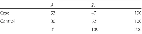
mAssocTest2G, the extension ofmTDT2Gto be applied in case/control GWAS, is defined as:
mAssocTest2G= (
ncas−g1−ncont−g1)2 ng1
+(ncas−g2−ncont−g2)2 ng2
,
with ncas−g1, ncont−g1 defined respectively as the
num-ber of cases and control haplotypes belonging to group g1. In a similar way, ncas−g2, ncont−g2 are also defined. ng1 is the total count of haplotypes in g1 and ng2 the
Table 8UnderstandingmAssocTest2G(II): haplotype counts from
the other half of the data set are to be used to compute the statistic
g1 g2
Case 53 47 100
Control 38 62 100
91 109 200
total count of haplotypes in g2. As with mTDT2G, the data set, the training data set in our case, is divided into two equally-sized parts for test application: one part is used to comprise the two groups and the other to com-pute the statistic.mTDT2G is aχ2test with 2 degrees of freedom.
For a better understanding of howmAssocTest2Gis com-puted, let us consider Table 7 of haplotype counts of length 3 obtained from half of a data set analyzed with 100 individuals. For the sake of simplicity, major and minor alleles at all loci are represented as 1 and 0, respectively.
From this table, group g1 comprises the haplo-types that are more frequent in cases than in con-trols: g1 = {000, 011, 101, 110}, and therefore all the
remaining haplotypes comprise the second group:g2 = {001, 010, 100, 111}. From these two groups, the second data subset is used to compute the statistic. Table 8 shows haplotype counts for the two groups from the second data subset.
Thus,mAssocTest2G= (53−38)
2+(47−62)2
200 = 22591 + 225109 = 4.5368 andp-value isp=0.033175.
In the third step, once we had computedmAssocTest2G on the training data set for sliding windows with an off-set of 1 and different haplotype lengths (from 1 to 5), we applied different levels of loci filtering (the 13 p -value upper limits previously mentioned) in order to select the input variables of the haplotype-based predictor of individual riskpIndh(i).
In the fourth step, we learned the predictors using all of the previously mentioned approaches from the second half of the training data set, i.e. those individuals used to compute themAssocTest2Gstatistic. The haplotype-based predictor is defined on the basis of a predictor of haplo-type risk,pHap(h). The log odds for each genome-wide homologous chromosome of an individual are therefore combined in order to estimate its individual risk. Each genome-wide homologous chromosome comprises one of the two chromosomes for each 22 chromosome pair. The input variables for the predictor of haplotype risk are binary ones, representing whether a haplotype belongs to g1 or g2. The output variable for the predictor of hap-lotype risk is the probability of a given genome-wide haplotype to be a high-risk haplotype. We consider that both genome-wide haplotypes comprising the genome of an unaffected individual must be low-risk haplo-types while both genome-wide haplohaplo-types comprising the genome of a diseased individual must be high-risk ones. Only individuals in the second half of the training data set (i.e. those used to compute the statistic) are used to build the haplotype risk predictor.
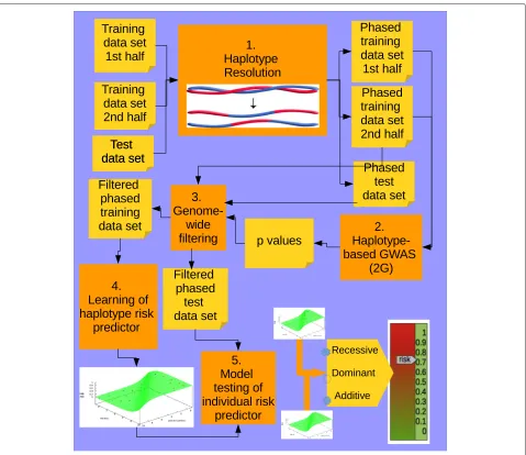
In the fifth and final step, we used the predictors to mea-sure their generalization capacity, by feeding them with individuals from the test data set. It should be noted that for small data sets and haplotypes comprising a few posi-tions there may be variants in the test data set that are not present in the training data set. In order to decide whether a haplotype at a given sliding window was a high (1) or low (0) risk one, we computed the similarity between it and each haplotype in the list of high risk and low risk haplo-types for the corresponding sliding window in the training data set. We therefore classified it as 1 or 0 depending on whether the closest haplotype belonged to the set of high or low risk haplotypes, respectively [31]. We used the length measure as the similarity measure [44], which computes the largest number of consecutive matching alleles. Figure 6 summarizes the entire procedure of our haplotype-based approach.
Additional file
Additional file 1: Supplementary material [45].(PDF 502 kb)
Competing interests
The authors declares that they have no competing interests.
Authors’ contributions
VP and MA conducted the experimental analyses. All the authors contributed to the writing of the manuscript. All authors read and approved the final manuscript.
Acknowledgments
This work was supported by the Spanish Secretary of Research, Development and Innovation [TIN2010-20900-C04-1]; the Spanish Health Institute Carlos III [PI13/02714]and [PI13/01527] and the Andalusian Research Program under project P08-TIC-03717 with the help of the European Regional Development
Fund (ERDF). The authors are very grateful to the reviewers, as they believe that their comments have helped to substantially improve the quality of the paper.
Author details
1Departamento de Lenguajes y Sistemas Informáticos, ETSIIT, c/ Periodista
Daniel Saucedo Aranda s/n Universidad de Granada, Granada 18071, Spain. 2Instituto de Parasitología y Biología Molecular, CSIC, Granada, Spain.
Received: 13 October 2014 Accepted: 27 November 2015
References
1. Jager PD, Chibnik L, Cui J, Reischl J, Lehr S, Simon KC, et al. Integration of genetic risk factors into a clinical algorithm for multiple sclerosis susceptibility: a weighted genetic risk score. Lancet Neurol. 2009;8(12):1111–9.
2. Evans D, Visscher P, Wray N. Harnessing the information contained within genome-wide association studies to improve individual prediction of complex disease risk. Hum Mol Genet. 2009;18:3525–31.
3. Chen H, Poon A, Yeung C, Helms C, Pons J, Bowcock AM, et al. A genetic risk score combining ten psoriasis risk loci improves disease prediction. 2011;6(4):e19454.
4. Li H, Yang L, Zhao X, Wang J, Qian J, Chen H, et al. Prediction of lung cancer risk in a Chinese population using a multifactorial genetic model. BMC Med Genet. 2012;13:118.
5. Brautbar A, Pompeii LA, Dehghan A, Ngwa JS, Nambi V, Virani SS, et al. A genetic risk score based on direct associations with coronary heart disease improves coronary heart disease risk prediction in the
Atherosclerosis Risk in Communities (ARIC), but not in the Rotterdam and Framingham Offspring, Studies. Atherosclerosis. 2013;223(2):421–26. 6. Demirkan A, Penninx BWJH, Hek K, Wray NR, Amin N, Aulchenko YS,
et al. Genetic risk profiles for depression and anxiety in adult and elderly cohorts. Mol Psychiatry. 2011;16(7):773–83.
7. Wang JH, Pappas D, Jager PLD, Pelletier D, de Bakker PI, Kappos L, et al. Modeling the cumulative genetic risk for multiple sclerosis from genome-wide association data. Genome Med. 2011;3:3.
8. Chibnik LB, Keenan BT, Cui J, Liao KP, Costenbader KH, Plenge RM, et al. Genetic risk score predicting risk of rheumatoid arthritis phenotypes and age of symptom onset. PLoS ONE. 2011;6(9):e24380.
9. Pospiech E, Draus-Barini J, Kupiec T, Wojas-Pelc A, Branicki W. Prediction of eye color from genetic data using Bayesian approach. Forensic Sci. 2012;57(4):880–6.
10. Sebastiani P, Solovieff N, Dewan A, Walsh KM, Puca A, Hartley SW, et al. Genetic signatures of exceptional longevity in humans. PLoS ONE. 2012;7:e29848.
11. Kooperberg C, LeBlanc M, Obenchain V. Risk prediction using genome-wide association studies. Genet Epidemiol. 2010;34:643–52. 12. Spiliopoulou A, Nagy R, Bermingham ML, Huffman JE, Hayward C,
Vitart V, et al. Genomic prediction of complex human traits: relatedness, trait architecture and predictive meta-models. Hum Mol Genet. 2015;24(14):4167–82. doi:10.1093/hmg/ddv145.
13. Wray N, Yang J, Goddard ME, Visscher PM. The genetic interpretation of area under the ROC curve in genomic profiling. PLoS Genet. 2010;6: e1000864.
14. Ripatti S, Tikkanen E, Orho-Melander M, Havulinna AS, Silander K, Sharma A, et al. A multilocus genetic risk score for coronary heart disease: case-control and prospective cohort analyses. Lancet. 2010;376(9750): 1393–400.
15. Myocardial-Infarction-Genetics-Consortium. Genome-wide association of early-onset myocardial infarction with single nucleotide polymorphisms and copy number variants. Nat Genet. 2009;41:334–41.
16. Hernesniemi JA, Seppälä I, Lyytikäinen LP, Mononen N, Oksala N, Hutri-Kähönen N, et al. Genetic profiling using genome-wide significant coronary artery disease risk variants does not improve the prediction of subclinical atherosclerosis: the cardiovascular risk in young finns study, the bogalusa heart study and the health 2000 survey – a meta-analysis of three independent studies. PLoS ONE. 2012;7:e28931.
18. Wei Z, Wang K, Qu HQ, Zhang H, Bradfield J, Kim C, et al. From disease association to risk assessment: an optimistic view from genome-wide association studies on type 1 diabetes. PLoS Genet. 2009;5:e1000678. 19. Grassmann F, Fritsche L, Keilhauer C, Heid IM, Weber BH. Modelling the
genetic risk in age-related macular degeneration. PLoS ONE. 2012;7(5): e37979.
20. Janssens A, van Duijn C. Genome-based prediction of common diseases: advances and prospects. Hum Mol Genet. 2008;17(Review Issue 2): R166–R173.
21. Jakobsdottir J, Gorin MB, Conley Y, Ferrell RE, Weeks DE. Interpretation of genetic association studies: markers with replicated highly significant odds ratios may be poor classifiers. PLoS Genet. 2010;5(2):e1000337. 22. Ribeiro RJT, Monteiro CPD, Azevedo ASM, Cunha VF, Ramanakumar AV,
Fraga AM. Performance of an adipokine pathway-based multilocus genetic risk score for prostate cancer risk prediction. PLoS ONE. 2012;7(6):e39236.
23. Jo J, Nam CM, Sull JW, Yun JE, Kim SY, Lee SJ. Prediction of colorectal cancer risk using a genetic risk score: the Korean cancer prevention study-II (KCPS-II). Genomics Inform. 2012;10(3):175–83.
24. Kang J, Kugathasan S, Georges M, Zhao H, Cho JH, NIDDK IBD Genetics Consortium. Improved risk prediction for Crohn’s disease with a multi-locus approach. Hum Mol Genet. 2011;20(12):2435–42.
25. Sebastiani P, Solovieff N, Sun JX. Naïve Bayesian classifier and genetic risk score for genetic risk prediction of a categorical trait: not so different after all! Front Genet. 2012;3:26.
26. Kang J, Cho J, Zhao H. Practical issues in building risk-predicting models for complex diseases. J Biopharm Stat. 2010;20(2):415–40.
27. Barrett J, Clayton D, Concannon P, Akolkar B, Cooper JD, Erlich HA. Genome-wide association study and meta-analysis find that over 40 loci affect risk of type 1 diabetes. Nat Genet. 2009;41(6):703-7.
28. Torres-Sánchez S, Medina-Medina N, Montes-Soldado R, Masegosa AR, Abad-Grau MM. Riskoweb: Web-based genetic profiling to complex disease using genome-wide snp markers In: Rocha MP, Corchado JM, Fdez-Riverola F, Valencia A, editors. Proceedings of the 5th International Conference on Practical Applications of Computational Biology & Bioinformatics (PACBB 2011). Berlin Heidelberg: Springer; 2011. p. 1–8. 29. Abad-Grau M, Medina-Medina N, Montes-Soldado R, Matesanz F,
Bafna V. sample reproducibility of genetic association using different multimarker TDTs in genome-wide association studies: characterization and a new approach. PLoS ONE. 2012;7(2):e29613.
30. Jostins L, Barrett JC. Genetic risk prediction in complex diseases. Hum Mol Genet. 2011;20(R2)(Review Issue 2):R182–8.
31. Abad-Grau M, Medina-Medina N, Masegosa A, Moral S.
Haplotype-based classifiers to predict individual susceptibility to complex diseases: An example for Multiple Sclerosis In: Schier J, Correia CMBA, Fred ALN, Gamboa H, editors. Proceedings of the International Conference on Bioinformatics Models, Methods and Algorithms. Setúbal, Portugal: SciTe; 2012. p. 360–6.
32. Janssens A, Moonesinghe R, Yang Q, Steyerberg EW, van Duijn CM, Khoury MJ. The impact of genotype frequencies on the clinical validity of genomic profiling for predicting common chronic diseases. Genet Med. 2007;9(8):528–35.
33. Freund Y, Schapire RE. Experiments with a new boosting algorithm. In: Proceedings of the Thirteenth International Conference on Machine Learning. San Francisco, California: Morgan Kaufmann; 1996. p. 148–56. 34. Hoerl AE, Kennard RW. Ridge-regression: biased estimation for
nonorthogonal problems. Technometrics. 1970;12:55–67.
35. Tibshirani R. Regression shrinkage and selection via the lasso. J R Stat Soc: Series B. 1996;67:91–108.
36. IMSGC I. Evidence for polygenic susceptibility to multiple sclerosis - the shape of things to come. Am J Hum Genet. 2010;86:621–5.
37. Purcell S, Neale B, Todd-Brown K, Thomas L, Ferreira MA, Bender D. PLINK: a tool set for whole-genome association and population-based linkage analyses. Am J Hum Genet. 2007;81:559–75.
38. Abad-Grau M, Montes-Soldado R, Sebastiani P. Building chromosome-wide LD maps. Bioinformatics. 2006;22(16):1933–4. 39. The-Wellcome-Trust-Case-Control-Consortium. Genome-wide
association study of 14,000 cases of seven common diseases and 3,000 shared controls. Nature. 2009;447:661–78.
40. Vapnik V. The Nature of Statistical Learning Theory. New York: Springer; 1999.
41. Hall M, Frank E, Holmes G, Pfahringer B, Reutemann P, Witten IH, et al. The WEKA data mining software: an update. SIGKDD Explorations. 2009;11:10–8.
42. Quinlan R. C4.5: programs for machine learning. San Francisco, California: Morgan Kaufmann; 1993.
43. Delaneau O, Zagury J, Marchini J. Improved whole chromosome phasing for disease and population genetic studies. Nat Methods. 2013;10:5–6. 44. Tzeng J, Devlin B, Wasserman L, Roeder K. On the identification of
disease mutations by the analysis of haplotype similarity and goodness of fit. Am J Hum Genet. 2003;72:891–902.
45. Cooper GF, Hennings-Yeomans P, Visweswaran S, Barmada M. An Efficient Bayesian Method for Predicting Clinical Outcomes from Genome-Wide Data. In: AMIA Annu Symp Proc. 2010. Bethesda, Maryland: AMIA; 2010. p. 127–31.
• We accept pre-submission inquiries
• Our selector tool helps you to find the most relevant journal
• We provide round the clock customer support
• Convenient online submission
• Thorough peer review
• Inclusion in PubMed and all major indexing services
• Maximum visibility for your research
Submit your manuscript at www.biomedcentral.com/submit