OASIS4 – a coupling software for next generation earth system modelling

(1)

www.geosci-model-dev.net/3/87/2010/

Geoscientific

Model Development

OASIS4 – a coupling software for next generation earth

system modelling

R. Redler1,*, S. Valcke2, and H. Ritzdorf1,**

1_{NEC Research Laboratories, NEC Europe Ltd., Sankt Augustin, Germany} 2_{CERFACS, Toulouse, France}

*_{now at: Max-Plack-Institute for Meteorology, Hamburg, Germany} **_{now at: NEC Deutschland GmbH, D¨usseldorf, Germany}

Received: 19 June 2009 – Published in Geosci. Model Dev. Discuss.: 7 July 2009

Revised: 17 November 2009 – Accepted: 19 December 2009 – Published: 22 January 2010

Abstract. In this article we present a new version of the Ocean Atmosphere Sea Ice Soil coupling software (OASIS4). With this new fully parallel OASIS4 coupler we target the needs of Earth system modelling in its full com-plexity. The primary focus of this article is to describe the design of the OASIS4 software and how the coupling soft-ware drives the whole coupled model system ensuring the synchronization of the different component models. The ap-plication programmer interface (API) manages the coupling exchanges between arbitrary climate component models, as well as the input and output from and to files of each indivi-dual component. The OASIS4 Transformer instance per-forms the parallel interpolation and transfer of the coupling data between source and target model components. As a new core technology for the software, the fully parallel search algorithm of OASIS4 is described in detail. First bench-mark results are discussed with simple test configurations to demonstrate the efficiency and scalability of the software when applied to Earth system model components. Typically the compute time needed to perform the search is in the order of a few seconds and is only weakly dependant on the grid size.

1 Introduction

Global coupled models (GCMs) have been used for climate simulations since the late 1960s starting with the pioneering work by Manabe and Bryan (1969). With advances in com-puting power, coupled models have been in use for century-long simulations since the late 1980s. Since that time, we

Correspondence to: R. Redler ([email protected])

observe a rapid and continuous increase of activity in global coupled modelling as additional computer resources have be-come available. Climate models can be considered as multi-disciplinary or multi-physics software tools to simulate the interactions of the atmosphere, oceans, land surface, sea ice and other components of the climate system. They are used for a variety of purposes from studies of the dynamics of the weather and climate system to projections of future climate. These models can range from relatively simple to quite com-plex, that is from zero-dimensional models and Earth-system Models of Intermediate Complexity (EMIC) to complex 3-D Global Climate Models (GCM) and Regional Climate Mo-dels (RCM).

A GCM aims to describe geophysical flow by integrat-ing a variety of fluid-dynamical, chemical, or even biological equations that are either derived directly from physical laws (for example Newton’s law) or constructed by more empiri-cal means. Classiempiri-cally, the two main constituents of a GCM are atmospheric and ocean circulation models. When cou-pled together (along with other components such as a sea ice model and a land model) an ocean-atmosphere coupled general circulation model forms the basis for a full climate model. A very recent trend in GCMs is to extend these tra-ditional coupled climate models to become full Earth system models (ESM), by including further model components to calculate atmospheric chemistry, marine biology or a carbon cycle model (matter cycle in a more general sense) to more correctly simulate the interaction between the different sub-components. Typically, these different model components are developed independently by different research groups.

Numerical modelling in its full complexity is still in its infancy, primarily due to the immense complexity of the task and insufficient empirical knowledge of many aspects of climate related processes. This is not only the case for the

(2)

oceans where in particular the knowledge of the subsur-face circulation is rather poor, but also for the hydrolo-gical cycle where precipitation, evaporation and the three-dimensional distribution of water vapour and clouds are in-sufficiently known. Despite these uncertainties the devel-opment of global climate models is one of the main unify-ing components in the World Climate Research Programme (WCRP) of the World Meteorological Organisation (WMO). The output of these models is considered as fundamental deliverables from the whole WCRP and provides the basis for the understanding and prediction of natural and human-made climate variations (CLIVAR Scientific Steering Group, 1998).

In the past, the important role of climate models has been addressed in a variety of research programmes on a global scale like the Climate Variability programme (CLIVAR) or the Coupled Model Intercomparison Project (CMIP) as one of the CLIVAR initiatives, while EuroCLIVAR, the Baltic Sea Experiment (BALTEX) or the North American Regional Climate Change Assessment Program (NARCCAP) focused on a regional scale. Most important, global climate models form one of the backbones of the Assessment Reports (AR) published by the Intergovernmental Panel of Climate Change (IPCC).

In addition to the model components used in an ESM, each community representing one of the physical components still feels a strong need for having separate stand-alone special-purpose versions of the individual components of the cou-pled climate models. These are used to investigate processes in the different subsystems and to test new physical parame-terisations in controlled scenario runs. The existence of dif-ferent research objectives and the need to estimate model uncertainty from model intercomparison (like for the IPCC AR) support the idea of a multi-component approach and the need for the interoperability of the different components. To achieve this interoperability, two approaches are nowadays considered: either some standard programming rules are fol-lowed by all component developer groups and the result-ing components are integrated into a sresult-ingle application, or the component models independently developed remain sep-arate applications and an external coupling software ensuring the lowest possible degree of interference in the component codes is used. As the first approach is almost impossible to apply when confronted with the heterogeneous development environment in Europe, we offer, with the OASIS4 coupler described in this paper, an implementation of the second ap-proach.

With OASIS4, we continue the software development of the Ocean Atmosphere Sea Ice Soil (OASIS) coupling soft-ware which has its origins in the early nineties at the Eu-ropean Centre for Research and Advanced Training in Sci-entific Computing (CERFACS, Toulouse, France). With the emerging complexity of ESMs, their increasing size (with re-spect to the number of grid points to be treated) and higher degree of parallelism, the limitations of OASIS3 (Valcke,

2006) and its predecessors have become visible and the need has emerged to provide the ESM community with new fully parallel coupling software. The development of OASIS4 started during the Program for Integrated Earth System Mod-elling (PRISM) project funded by the European Commission from 2001 to 2004. PRISM (Valcke et al., 2007) was or-ganized by the European Network for Earth System Mod-elling (ENES), and is currently continuing within the new Framework 7 Programme funded by the European Commis-sion with the IS-ENES (Infrastructure for the European Net-work for Earth System modelling) project.

At the time when the OASIS4 development started, cou-pling software performing field transformation already ex-isted, such as the Mesh based parallel Code Coupling Inter-face (MpCCI) (Joppich and K¨urschner, 2006) or the Com-munity Climate System Model (CCSM) Coupler 6 (Cpl6) (Buja and Craig, 2002). MpCCI is not available as source code, and for this particular reason the MpCCI software has not been accepted by the ESM community. With new ver-sions of the MpCCI software its developers have abandoned some important aspects of parallelism. Compared to previ-ous versions all grid information is now assembled in a sin-gle MpCCI coupler instance for performing the neighbour-hood search and regridding. This approach makes it even less attractive for the usage within an ESM with a high de-gree of parallelism. The concept of CCSM and Cpl6 is very much similar to OASIS4. However, earlier versions of Cpl6 have targeted the specific needs of the CCSM and the cou-pler could only be executed within the complete CCSM. The Earth System Modelling Framework (ESMF) software en-vironment (Hill et al., 2004) provides an implementation of the first interoperability approach described above. ESMF is a high-performance software infrastructure that can be used to build a complex application as a hierarchy of individual units, each unit having a coherent function, like modelling a physical phenomenon or managing the input and output (IO), and a standard calling interface. While an ESMF application, being more integrated, will most probably be more efficient compared to an OASIS4 coupled system, ESMF may require a deeper level of intervention in the application code. For example, ESMF requires that components be split into ini-tialize, run, and finalize sections, with each callable as a sub-routine. Necessary modifications of the software to achieve the full benefit from ESMF is described briefly by (Hill et al., 2004). In contrast to ESMF, the OASIS4 application pro-grammer interface (API) can be integrated with only minor modifications in the original application code, and is for this particular reason more attractive to the European ESM com-munity with its less centralised modelling efforts.

(3)

regarding the coupling of physical quantities remains under the full responsibility of the application code. In compensa-tion, the flexibility of OASIS4 provides the ESM community with the ability to couple a wide range of ESM components. With this article we address the questions we have received from the growing user community during the last couple of years. The originality of OASIS4 relies in its great flexi-bility which is explained in Sects. 2–4, where the software design ideas, the driving and configuration mechanisms and the application programmer interface to the communication library are detailed. Another new concept introduced with OASIS4 is the parallel 3-D neighbourhood search and regrid-ding based on the geographical description of the process lo-cal domains (see Sects. 5 and 6). The data flow, in particular the common treatment of coupling and IO exchanges (a con-cept already available with OASIS3) is briefly described in Sect. 7.

We conclude the technical description with first perfor-mance measurements shown in Sect. 8 and outlook to on-going and future work in Sect. 9.

2 General design and overview

The key concept behind the OASIS4 software is to provide a tool to the ESM community which is portable to any existing computing environment. Mainly this is achieved by adhering to programming standards that have emerged over time. For a complete list of systems and environments which are sup-ported by OASIS4, the reader is invited to visit the OASIS4 Wiki page1.

The OASIS4 software package provides the source code for a Driver-Transformer executable and a library (called PSMILe hereafter). At run-time, the OASIS4 Driver-Transformer and the component models remain separate (possibly parallel) executables. To communicate with the rest of the coupled system, each component model needs to be linked against the PSMILe. To be as user-friendly as possible, the PSMILe API includes a limited number of re-quired function calls, at the same time supporting all typical ESM component data structures. While it is not designed to handle the component internal communication, the library completely manages the coupling data exchanges with other model components and the details of the I/O file access. In this article, we will use the term “coupled application” to de-scribe the ensemble formed by the component models cou-pled through the OASIS4 Driver-Transformer.

The major task of OASIS4 is to handle the data exchange between ESM components. These exchanges are completely built upon the Message Passing Interface (MPI) (Snir et al., 1998; Gropp et al., 1998). The major justification for this decision is the fact that MPI has become a quasi standard to handle parallel applications. MPI libraries are available on

1_{https://oasistrac.cerfacs.fr/}

almost every parallel architecture, be it a vendor-specific im-plementation or provided as one of the many publicly avail-able MPI packages. The complexity of MPI is nevertheless hidden behind the OASIS4 API.

In contrast to previous versions of OASIS, the coupled configuration has to be described by the user with the help of Extentable Markup Language2 (XML) files. In order to read in this information, linking to an XML library is re-quired. Similar to OASIS3, NetCDF (Rew and Davis, 1997) file IO is supported to optionally read and write forcing in-put, diagnostic output and coupling restart files; in this case, a NetCDF or a parallel NetCDF (Li et al., 2003) library needs to be provided. Last but not least, compilers conform to pub-lished Fortran90 and C language standards are required.

With the current version, bilinear, trilinear, bicubic and nearest-neighbour parallel interpolation is provided for the most prominent grid types used in ESM components to map the source grid values to the target grid in a data exchange. Furthermore, 2-D conservative remapping is available which is usually the preferred way to regrid fluxes.

In particular, OASIS4 supports 2- and 3-D coupling be-tween any combination of logically-rectangular, i.e. 2-D structured, or Gaussian Reduced grids in the horizontal longitude-latitude plane, each horizontal layer repeating it-self at different vertical levels. OASIS4 is also able to han-dle the exchange of non-geographical data, i.e. data which are solely provided in an (i, j, k) index space not associ-ated to any geographical domain. To properly handle non-geographical data, it is required that the pairs of source and target grids work over the same global index range, although the data can be partitioned differently on the source and tar-get side.

3 The driving and configuration mechanisms

The OASIS4 Driver-Transformer executable can consist of one or more processes. During the initialisation, the root process of this instance acts as a Driver while during the in-tegration of the coupled model the root and additional pro-cesses act as Transformer propro-cesses performing the regrid-ding of the coupling fields. The Transformer task is further discussed in Sects. 6 and 8. In this section we focus on the Driver aspect.

OASIS4 supports two ways of starting a coupled appli-cation. With a complete implementation of the MPI2 stan-dard, only the Driver processes have to be started by the user. All remaining physical components are then spawned by the OASIS4 Driver at run time. In this scenario, no ex-tra programming work has to be invested in the component internal parallelisation as any original MPI communication will work as is. If the available MPI library does not sup-port the MPI2 standard, all processes of the whole coupled

2_{http://www.w3.org/XML/}

(4)

application will have to be started simultaneously in a “multi-ple program multi“multi-ple data” (MPMD) mode; the disadvantage of this approach is that each component must use a specific MPI communicator for its own internal communication. This MPI communicator is created and provided by the OASIS4 software.

The whole coupled configuration is described with the help of XML files. XML is a simple, very flexible text for-mat. Originally designed to meet the challenges of large-scale electronic publishing, XML is also playing an increas-ingly important role in the exchange of a wide variety of data on the Web and elsewhere. An XML document is simply a file which follows the XML format. The OASIS4 configu-ration XML files must be created by the coupled model de-veloper. A Graphical User Interface (GUI) is currently being developed to facilitate the creation of those files.

The “Specific Coupling Configuration” (SCC) XML file defines the general characteristics of a coupled model run, for example the components to be coupled and the number of processes for each component. The Specific Model Input and Output Configuration (SMIOC) XML files (one for each component) describes the relations each component model will establish with the external environment through inputs and outputs for a particular run. In the SMIOC files, the user specifies the coupling exchanges, for example the source or target of each input or output field (either another component or a disk file), the exchange frequency, and the transforma-tions to be performed by OASIS4 on this field.

The contents of the XML files are read and interpreted by the Driver, and information relevant for the physical compo-nents is communicated to the respective PSMILe and Trans-former processes on case-by-case basis.

4 The application programmer interface

In this section, we briefly describe the design ideas of the OASIS4 API to the PSMILe and highlight the differences compared to OASIS3.

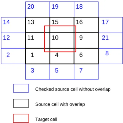
The API function calls (see Table 1) can be split into three different phases. During the initialisation phase, some ba-sic initialisation routines must be called and the grid and ex-change fields need to be specified to the PSMILe. The initial-isation phase is concluded with a call to PRISM Enddef (see Sect. 5). The second phase comprises the exchange of data further described in Sect. 7 while the third phase denotes the termination of the coupling. For a detailed description of the OASIS4 API, we refer the reader to the OASIS4 User Guide (Valcke and Redler, 2006).

4.1 General design

The general design follows several principles. First, the PSMILe API routines that are defined and implemented shall not be subject to modifications between the different versions

of the OASIS4 software. However, new routines may be added in the future to support new functionality. In addition, the PSMILe has been kept extendable to new types of cou-pling data and new types of grids by using Fortran90 func-tion overloading. Some complexity of the API arises from the need to transfer not only the coupling data but also the associated metadata, i.e. mainly the information about the associated grid. We carefully selected the necessary argu-ments for each subroutine in order to keep the argument lists as short as possible. At the same time we kept the interfaces generic in order to avoid the introduction of another set of routine for every new configuration we have to support with the software.

Like in the MPI, the memory that is used for storing in-ternal representations of various data objects is not directly accessible by the user and the objects can only be addressed indirectly by the component via their handle. Handles are of type integer and represent an index to an entry in a list of the respective objects. The object and its associated handle are significant only on the process where it is created.

Furthermore, the internal usage of MPI is completely hid-den from the user, except when the available MPI library does not offer the MPI2 spawning functionality (which im-plies that all processes have to be started simultaneously in an MPMD mode, see Sect. 3). In this case, each component has to retrieve a special MPI communicator for its internal communication which is created by the PSMILe and acces-sible with a specific function call to PRISM Get localcomm (see Table 1); this call remains the only MPI-related call.

When using MPI for internal communication in paral-lelised components, the calling sequence of some MPI-and PRISM-related calls has to follow a certain rule which is sketched in Fig. 1. The function calls to PRISM Init and PRISM Init comp can be used as a full substitute of MPI Init, while the PRISM Terminate can be used as a full substitute for MPI Finalize.

4.2 Data exchanges

(5)

Table 1. List of OASIS4 PSMILe function calls. Description of the OASIS4 PSMILe Function Calls.

Name Description

Initialisation PRISM Init Initialisation of the application

PRISM Init comp Initialisation of a component within an application PRISM Def grid Abstract definition of a compute grid

PRISM Def partition Definition of the process-local grid partition relative to the global compute domain PRISM Reducedgrid map Additional information needed for Gauss-reduced grids

PRISM Set corners Definition of geographical positions of vertices of grid cells PRISM Set mask Definition of masked points or cells

PRISM Set points Definition of geographical positions of points PRISM Def var Definition of exchange and IO fields

PRISM Enddef End of the definition phase

Data Exchange

PRISM Get To receive data from a remote component and/or read in from a file PRISM Put To send data to a remote component and/or write into a file PRISM Put restart To write additional data sets into an OASIS4 coupling restart file

Termination PRISM Terminate Termination of the prism part

Auxiliary and Query Functions

PRISM Calc newdate Add and Subtract operations on the OASIS4 Fortran90 Time structure PRISM Get localcomm To retrieve a MPI communicator for component local communciation PRISM Initialized To check whether PRISM Init has already been called

PRISM Put inquire A query function to obtain information whether a PRISM Put has to be posted PRISM Terminated Query function to check whether PRISM Terminate has already been called

PRISM Abort To terminate the coupled application in a well defined to support user-defined error handling

The sending and receiving PSMILe PRISM Put- and PRISM Get calls can be placed anywhere in the source and target code and possibly at different locations for the dif-ferent coupling fields. These routines can be called by the model at each timestep. The actual date at which the call is performed and the date bounds for which it is valid are given as arguments; the sending/receiving is effectively per-formed only if the date and date bounds correspond to a time at which it should be activated, given the field coupling or IO dates indicated by the user in the SMIOC; a change in the coupling or IO dates is therefore also totally transparent for the component model itself.

When the action is activated at a coupling or IO date, each process sends or receives only its local partition of the data, corresponding to its local grid defined previously. The cou-pling exchange, including data repartitioning if needed, then occurs, either directly between the component models, or via additional Transformer processes if regridding is needed.

If the user specifies that the source of a PRISM Get or the target of a PRISM Put is a disk file, the PSMILe exploits the GFDL mpp io package (Balaji, 2001) for its file IO (see Sect. 7 for more detail).

PRISM Init comp

...

PRISM Terminate

PRISM Init

PRISM Init comp

...

PRISM Terminate

MPI Init

PRISM Init comp

...

PRISM Terminate

MPI Finalize

MPI Init

PRISM Init

PRISM Init comp

...

PRISM Terminate

MPI Finalize

Fig. 1. The four allowed sequences of calls for initializing and terminating an ESM component for coupling with OASIS4 and its relation to MPI.

32

Fig. 1. The four allowed sequences of calls for initializing and

ter-minating an ESM component for coupling with OASIS4 and its re-lation to MPI.

(6)

4.3 OASIS3 and OASIS4 APIs

The major difference between the OASIS3 and OASIS4 APIs from a user point view is in the initialisation phase. In OASIS3, the global grid information has to be provided in separate OASIS3 specific NetCDF grid files which are ac-cessed by OASIS3 routines. With OASIS4 it is assumed that each component has all knowledge about its own local geo-graphical grids at some point during the initialisation phase. This local grid information has to be provided through the API to initialise the PSMILe search.

Beside this difference, we have kept the design of the OASIS3 and OASIS4 PSMILe API as similar as possible, both following in particular the principle of “end-point” data exchange explained above, in order to allow an easy transi-tion from OASIS3 to OASIS4 for the community of users.

5 Neighbourhood search

The PSMILe library performs the exchanges of coupling data between source and target components. Usually those com-ponents express their coupling fields on different numeri-cal grids and a regridding operation has to be performed on the coupling data. The regridding implies: 1-identifying the “neighbours” of each target point, i.e. the source grid points that will contribute to the calculation of the target grid point value in the regridding process (in this article, we use the term “neighbourhood search” to describe this pro-cess), 2-calculating the weights of the different neighbours and 3-performing the calculation of the grid point values. To minimize the transfer of source data, it was decided to per-form the neighbour search (1) in the source PSMILe and to transfer only the useful source grid points (see Sect. 5.1 for further details) to the Transformer which performs the re-gridding calculation per se (i.e. 2 and 3). In this section, we describe the neighbourhood search performed by the source PSMILe.

The goal here is to provide a highly efficient search al-gorithm which determines the neighbourhood relations be-tween source and target grid points without generating sig-nificant overhead with respect to the model compute time. For ESMs the typical elapsed time for a job is in the order of hours and the search should not take more time than a few seconds. At the same time the algorithm has to rely on only a very limited number of a-priory assumptions in order to be flexible and applicable to more than just a few special grid configurations.

Compared to typical physical algorithms for numerical models, the result or the output of a search algorithm is al-ready well determined when the problem is posed, i.e. when the numerical grids are defined. For any given regridding scheme a unique solution exists regarding the neighbourhood between target and source points. When programming a li-brary for such purposes, the task is to have flexible

algo-rithms that are able to deal with any peculiarities of a given grid configuration. While an application programmer typi-cally has a complete control over the local grid, this is not the case for the library programmer as the library has to work based on the information provided through the user API without any or with only very limited a-priory assumptions.

In order to initialise the search, the components have to provide geographical information about the position of the grid points and about the reference volume or area that is associated with the grid points. This information is stored in one-dimensional arrays together with the grid type depen-dent shape of the original multidimensional array. The grid type and the information about the array shape provides the implicit knowledge about the connectivity of the grid points within a single block. Within these blocks correct neigh-bours have to be identified for each target point. In a sim-ple imsim-plementation of such search algorithm, this task can be achieved by comparing the distances for each target point with all source points available. This approach will be of the order of N2w.r.t. to the compute time (N being the number of target points to be processed, assuming that source and tar-get grids are about the same size). While such an approach may still be justified for small problem sizes, this approach will fail when the horizontal resolution is increased and grids become larger in size. For OASIS4, we have chosen a hierar-chical approach in order to minimise the workload during the search. We briefly describe here key aspects of the search al-gorithm which ensure its efficiency. An additional difficulty arises with parallelised components where the source grid is partitioned. For selected target points, the required “neigh-bour” source locations may reside on different processes and the search has to be extended across process boundaries. In the remaining part of this section we describe the different tasks which are performed by the PRISM Enddef call. 5.1 Point-based search for block-structured grids

(7)

is transmitted to the respective source process which shares a particular intersection. We note here that only the envelopes of all partitions are stored on all processes. For this and all following steps in the PSMILe or in the Transformer, it is never required to gather the global grid information at a cen-tral place onto one single process. This design aspect allows a minimal use of extra memory for the coupling operations.

The task of the second stage of the search is to find a re-ference source point for each target point which can later be used as a starting point to build the required interpolation stencil, i.e. the set of source neighbour points used for the calculation of the target point value, or to locate additional neighbours based on the user choice.

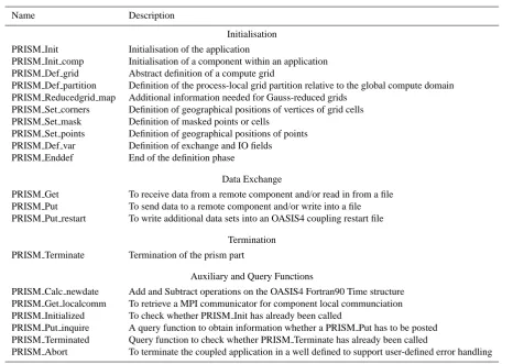
On the source side, a grid hierarchy is established out of the local source grid. For block-structured grids, this grid hierarchy is constructed by splitting the local source grid into smaller subsections with a refinement factor of two similar to a multi-grid approach (see Fig. 2). The subsection on the highest (finest) level in the grid hierarchy typically contains three grid points in each direction. For each target grid point in the list, we first determine the containing subsection on the lowest (coarsest) level by considering the bounding boxes of the subsections on this level. These bounding boxes are constructed by evaluating the minimum and maximum cell extent in a given i-j-k index range. This containing box is then subdivided into four subsections (or eight subsections in a 3-D search) on the next higher level, and those four or eight boxes are investigated in the same way. The process in continued until we have reached the highest level and are close to the required source point.

We note here that due to this simple approach based on bounding boxes, it is possible for any target point to be lo-cated in a region covered by more than one bounding box. We start the search in one of these boxes moving up to finer levels. The higher the levels are in our hierarchy the closer we can approximate the exact geometry of the local domain. It may happen that the algorithm does not find any appro-priate bounding box on a higher level. In such a case the algorithm jumps back to the previous lower level and contin-ues with another bounding box. These cycles are repeated until either a containing source cell is identified or until all bounding boxes under consideration have been investigated. At this stage, the search on the global domain is completed.

A great advantage of the multi-grid algorithm is that it is only weakly dependent on the problem size. When the grid size is doubled in each horizontal direction this would only introduce one more multi-grid level. For grids commonly used in climate modelling and for higher resolution grids, the overhead to set up the multi-grid hierarchy is more than compensated by the speedy search. OASIS4 is thus able to handle very large problem sizes (for example a global grid with 1/12◦horizontal resolution) in a reasonable amount of time. The performance of the OASIS4 multi-grid search is further discussed and compared with the performance of a classical search in Sect. 8.4.

overlap

Fig. 2. Sketch of a multi-grid hierarchy for a local domain.

Typi-cally the number of cells is much higher and the PSMILe will con-struct o(10) levels.

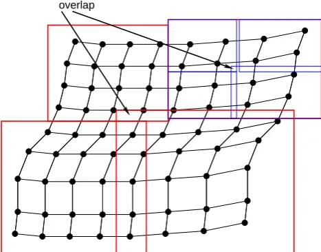
Now that the containing source cell is identified, the next step is to determine the reference source point. The source points are used to construct an auxiliary cell grid where the source points serve as corners of the cells (see dashed and solid lines in Fig. 3). The task is then to locate the source-point cell which contains the projection of the respective tar-get point. This is performed with a local search by investigat-ing each of the four source-point cells that surround the point which belongs to the containing source cell. In this example, the source-point box built with points at indices [i, j], [i+1, j], [i, j+1], and [i+1, j+1] is chosen and the source-cell of the point [i+1, j+1] (green box in Fig. 3) is found. This imme-diately directs us to identify the point with index [i, j] as the “lower-left” source-point. This location is now stored as the reference source point for the particular target point.

In the final step, the remaining source neighbours are iden-tified which are required to perform the interpolation re-quested by the user. For a bilinear interpolation, we are now able to identify the four corner points of the auxiliary cell (black open and solid bullets connected by solid lines) as the four neighbour source points needed. For a bicubic interpo-lation, sixteen neighbours have to be identified (the afore-mentioned bilinear points plus the open blue circles shown in Fig. 3).

Typically, block-structured grids include masked points in their compute domain. The algorithm as it is described so far does not distinguish between source masked and non-masked points but solely works on all grid coordinates in the source grid compute domain. For some target points, some source points first identified as neighbour points may not be avail-able for the interpolation if they are masked out which means that the physical fields do not necessarily contain meaningful values on those points. In such cases the user has different

(8)

i,j

i+1,j−1 i+2,j−1 i+1,j i+2,j i−1,j+2 i,j+2

i,j+1 i−1,j+1

i+1,j+2 i+2,j+2

i+1,j+1 i+2,j+1

i,j−1 i−1,j−1

i−1,j

Target Point

Reference Source Point

Associated cell area for point i+1, j+1

Additional source points for bilinear interpolation

Additional source points for bicubic interpolation

Fig. 3. Building the interpolation star based on the initial location.

choices via the XML configuration file. As a default op-tion, the remaining valid points will be used for a weighted-distance interpolation. Another option available is to not in-terpolate onto such target points. In the extreme case when all neighbour source points identified by the default search are masked, OASIS4 offers the possibility to search for the non-masked nearest-neighbour value and use this value for the target point. For this extra nearest-neighbour search, the algorithm starts from the original masked source grid point taken as an initial guess. Starting from the finest level con-taining the initial guess, the multi-grid hierarchy is then used again to locate the closest non-masked source points by mov-ing in so-called w-cycles through the multi-grid hierarchy, that is going down to a coarser level and going up again in another branch of the hierarchy repeatedly until the closest point is found.

5.2 Search on domain-partitioned source grids

On modern parallel systems, the application domain is usu-ally distributed to many processes and/or processors. If the interpolation of fields was performed using locally available data only, i.e. data which is available on the actual process, the result of the interpolation would depend on the actual partitioning. For example, if a target point is located close to the internal border of a partitioned domain of the source application, the standard interpolation stencil may require source points which are not located on the actual process but

which are located on a neighbour process. The PSMILe cur-rent search, called “global” search in the following, considers remote neighbour points appropriately, and therefore ensures that the interpolation is invariant to the domain partitioning.

The “global” search ensures that required data from source neighbour points located on remote processes is provided to-gether with local source data to the OASIS4 Transformer. Since the definition of application grids is quite general and since the full connectivity information for partitioned grids is not provided to the OASIS4 library (and is not explic-itly available in most of today’s climate model component codes), missing source points for interpolation stencils re-quire an additional search step. In this additional search step, the missing source points for the interpolation are searched in remote neighbouring domains. For block-structured grids, remote neighbouring domains are identified by exchanging information about the global index space provided through the PRISM Def Partition function call. If these remote source neighbour points are found, the full information in-cluding the mask data are returned to the process which has initiated this additional search step. At run-time, this process will collect the data from possibly different processes and will forward the data for the full interpolation to the Trans-former.

5.3 Point-based search for Gauss-reduced grids

(9)

5.4 Cell-based search

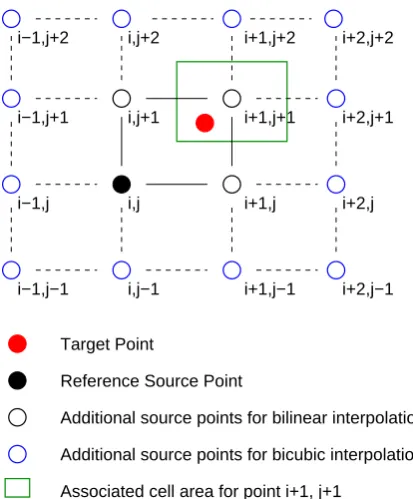
Compared to the search described above for point-based in-terpolation schemes, the cell-based search has to follow a slightly different approach. In order to determine all nec-essary information for conservative remapping, the task here is to locate, for each target cell, its overlapping source cells. In order to again reuse as much functionality as possible, we perform a point-based search on the corner coordinates in a very similar way to the search described above in order to ob-tain the start location. The indices that we obob-tain for the start location refer to the data structure of the corner points. For block-structured grids, these indices can easily be mapped to cell indices. The cell indices point us to the location of the geographical information of the cell corners (or vertices of the element). For each target cell, we can now use this initial source cell to continue the local search and identify the remaining source cells which overlap a given target cell (Fig. 4). The intersection or overlap between a pair of source and target cells is determined by a pairwise investigation of the intersection of the edges without a detailed evaluation of the exact area of overlap. The numbering shown in Fig. 4 indicates the order in which the local search is performed on the source grid. In this particular case, 21 cells are in-vestigated starting with the initial source cell 1. For each of the source cells, the overlap with the target cell is checked. Source cells with no overlap are marked as visited. Source cells that overlap with the target cell are marked and stored in memory. For an individual local search, the path way through the source cells is not fixed but dependent on the local prob-lem.

5.5 Optimisation

Most grids used in Earth system modelling are block-structured grids. Historically, codes have been developed for stand alone models with non-global grids in mind. Particular issues regarding the connectivity are handled internal to the code to the extent it is needed for the advection and diffusion operators and other boundary conditions. For global grids so-called cyclic boundary conditions have been introduced to guarantee a seamless continuation of the grid in the zonal di-rection. When approaching the geographical poles additional ghost-cells are introduced in order to properly calculate the operators along the zonal boundaries (see for example Madec and Imbard, 1996). When considering the i–j domain in the case of coupling, a target cell close to the pole may extend further than what is covered by the source ghost-cells in the i–j space. As the codes lack the information about the con-nectivity at the poles, in general, an additional search in the geographical domain is necessary. Not all of this implicit and sometime configuration specific information is transpar-ent for an external software package like the coupler. A new interface routine could be added to the API to transfer to the PSMIle any explicit connectivity information the

appli-Checked source cell without overlap

Source cell with overlap

Target cell

10

11

12

14

20

13

19

16

15

18

9

7

5

4

1

3

2

6

21

17

8

Checked source cell without overlap

Source cell with overlap

Target cell 10 11

12

14 13 15 16

9

7 5

4 1

3

2 6

21 17

8

Fig. 4. Search of source cells for conservative remapping.

Num-bers indicate the sequence in which the source cell are investigated locally.

cations would be able to provide. This would help to increase the efficiency of the search locally and across process bound-aries beyond what is achieved already today.

The OASIS4 PSMILe search algorithms are designed to work on 3-D model domains. In general, one could think about treating all grids as 3-D fully irregular or unstructured grids. In this way, one would ignore important a-priory in-formation useful to speed up the search process. In order to take advantage of the existing a-priory knowledge (in par-ticular about regularity along any of the grid axis), different grid types are introduced. The different vertical layers of grids with vertical z-coordinates are usually a simple vertical translation of the same 2-D horizontal grid. In such cases, the search is split into two parts with a 2-D search in the hor-izontal plane and a 1-D search along the vertical axis. In the horizontal plane, if the different columns or rows of the grid are respectively just a longitudinal or latitudinal translation of one same column or row, the search can be conducted by performing a 1-D search along each axis which further re-duces the compute time.

It is obvious that individual source points or cells are needed for the calculation of more than just one target grid point or cell. In order to minimize the amount of data to be transferred and stored, redundant geographical informa-tion (usually of type double precision or real) is removed and an index list is created to guarantee a well defined and cor-rect access to the geographical information. In order to allow the scattering onto the final n-dimensional destination array during the data exchange, these access index lists are also transmitted to the target process.

(10)

6 PSMILe-Transformer interaction and regridding

As outlined further in Sect. 7, the PSMILe supports two dif-ferent ways of exchanging data, directly between two compo-nents or through the Transformer processes when regridding is required. Here we concentrate on the latter case and de-scribe the transfer of information between the PSMILe and the Transformer and the regridding per se done on the cou-pling fields.

As the final result of the PSMILe search described in the last section, each source process holds 1-D lists, each list containing the geographical information relevant for the re-gridding of an intersection of the local source grid domain with one target process grid domain. As stated above, ac-cess index lists are created along with the raw geographi-cal information. Hereafter, we will geographi-call these lists “intersec-tion regridding lists”. These intersec“intersec-tion regridding lists are equally distributed over the Transformer processes available. This ensures that the Transformer processes work in parallel over the regridding of the different source and target process intersections.

During the run, the different Transformer processes wait for messages to arrive from any component process PSMILe, receive header messages containing information about the next message to receive or pending requests to fulfill, and perform related actions. They repeat this sequence of actions in an indefinite loop until the entire coupled run is finished. During the exchange phase, each Transformer process re-ceives the grid point field values (transferred from the source component code with a PRISM Put call) corresponding to its lists, calculates the regridding weights if it is the first ex-change, and applies the weights. The resulting target values are made available to the corresponding target PSMILe pro-cess. The data are sent upon request from the respective tar-get process (i.e. when a PRISM Get is called in the tartar-get component code).

The calculation of the weights depends on the regridding algorithm chosen by the user in the XML configuration file which can be different for each coupling field. The cur-rent version of OASIS4 supports purely 3-D regridding (3-D n-neighbour distance-weighted average or trilinear inter-polation) and 2-D regridding in the horizontal plane (2-D n-neighbour distance-weighted average, bilinear, bicubic in-terpolation or conservative remapping) followed by a linear interpolation in the vertical. As in OASIS3, the 2-D algo-rithms are taken from the Spherical Coordinate Remapping and Interpolation Package (SCRIP) library (see Jones, 1999). In particular, for the 2-D conservative remapping, the contri-bution of each source cell is proportional to the fraction of the target cell it intersects; this ensure local conservation of extensive properties such as fluxes. The 3-D algorithms are 3-D extensions of the 2-D SCRIP algorithms. For a detailed description of the regridding the reader is therefore referred to Jones (1999) and to the SCRIP User’s Guide (see Jones, 2001). As the SCRIP bicubic algorithm is based on the

func-tion gradient in the i and j direcfunc-tions, it cannot be applied for the Gauss-reduced grids. For those grids, the SCRIP func-tionality has therefore been extended by a standard bicubic algorithm based on the 16 source neighbours.

Analysing the quality of the regridding algorithm is a del-icate issue and no firm number can be given as the results depend on the source and target grids and on the character-istics of the regridded field. As an indication, we show here the error obtained when regridding the values of an analyt-ical cosine bell function which presents one minimum and one maximum over the global Earth domain. For longitude λand latitudeφthis is expressed as

F1=2−_cos[π·acos(cos(λ)cos(φ))]

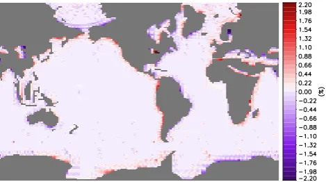
The relative error, i.e. the difference between the regridded value and the analytical value of the function divided by the analytical value, is calculated on each target grid point. The Figs. 5–8 present the results with each pixel showing exactly this relative error for each target grid point. No projection in the latitude-longitude space has been performed to avoid any additional interpolation by the graphic package.

Figure 5 shows the relative error obtained with the bilin-ear interpolation from the LMDz grid to the ORCA2 grid. LMDz (Hourdin et al., 2006) has a regular 3.75◦×2.535◦ grid. ORCA2 (Madec, 2008) is based on a 2◦Mercator mesh, (i.e. variation of meridian scale factor by cosine of the lati-tude); in the Northern Hemisphere the mesh has two poles so that the ratio of anisotropy is nearly one everywhere. The error is not shown for masked target points (grey areas). One can observe a relative error smaller than 0.4% over most of the domain. Near the coastline, for example near the west coast of the northern South America, the error can reach 0.8% at maximum. For those points near the coastline, some source points that are identified as bilinear neighbours are masked out. The remaining (non-masked) valid points are used for a less precise weighted-distance interpolation result-ing in a larger error.

(11)

Fig. 5. Relative error obtained (in %) with the bilinear regridding

from the LMDz grid to the ORCA2 grid.

Fig. 6. Relative error obtained (in %) with the bicubic regridding

from the Gauss-reduced grid to the ORCA2 grid.

Figure 7 shows the relative error obtained with the conser-vative remapping from the ORCA2 grid to the LMDz grid. The relative error is everywhere smaller than 0.2% except for the last row of the LMDz grid close to the North pole and near the coastline where it can reach respectively 1% and 2.2%. The SCRIP library assumes that the border of a cell between two cell corners is linear in longitude and latitude: near the North pole, this assumption becomes less valid and this can explain the larger error. Near the coastline, different normalisation options are available in the SCRIP library to calculate the value of the target cells which partially overlap masked source cells (see Jones, 2001). We chose the option to normalize by the area of the target cell intersecting non-masked source cells; this option does not locally conserve extensive properties but results in more realistic target values even if the error is still relatively large. With the alternative option, the normalisation by the full area of the target cell, the relative error (not shown) can become as large as 100%.

We note here that the data structure provided to the OASIS4 Transformer differs from the data structure sent to the OASIS3 Transformer. The source points that are used for a particular interpolation stencil may arrive in a differ-ent ordering. The data are multiplied with their individual weights and summed up. The different ordering during the

Fig. 7. Relative error obtained (in %) with the conservative

remap-ping from the ORCA2 grid to the LMDz.

Fig. 8. Relative error obtained (in %) with the bilinear regridding

from the LMDz grid to the ORCA2 grid when each component is partitioned over 3 processes and when the global search is not acti-vated.

summation may lead to truncation errors which become vis-ible when comparing the results obtained with OASIS3 and with OASIS4 even though both software use the same regrid-ding algorithms.

Finally, as an illustration of the benefits of the global search (see Sect. 5.2), Fig. 8 shows the relative error ob-tained with the bilinear interpolation from the LMDz grid to the ORCA2 grid when each component is partitioned over 3 processes (in the longitudinal direction) and when the global search is not activated. Comparing with Fig. 5, we observe greater relative error (of the order of 1% compara-ble to the maximum error obtained near the coastline) near the borders of the source partitions. This can be expected as for those target points the local search cannot find the usual 4 surrounding neighbours needed for the bilinear interpola-tion (as some of those 4 neighbours are located on a neigh-bour process domain). The remaining neighneigh-bours are used for a less precise weighted-distance interpolation resulting in a larger error. When the interpolation is performed with the global search described in Sect. 5.2, this greater relative error vanishes and regridded results (not shown) are exactly the same in the partitioned and not partitioned cases, which validates the global search.

(12)

7 Data exchange

The exchange of coupling data is typically happening inside a loop over time or iterations and is activated many times during the execution of the coupled model. Therefore the handling of the data exchange is a time-critical task. One of the major targets is to minimise the communication overhead and to avoid load-balancing problems induced by the imple-mentation of the exchange.

The data exchange is invoked by the component models using the PRISM Put and PRISM Get interface routines. These interface routines can be called individually by each model component at an arbitrary non-constant frequency. The coupling frequency is determined in the XML file at the beginning of the job. Inactive calls will return without per-forming any MPI calls. Only active prism calls (calls that are performed for a date at which an exchange has to occur) will call the MPI library to exchange data. OASIS4 verifies that the successive date bound arguments to these calls cover the run duration with no overlap and no gap and therefore takes care that the active calls have a one to one correspondence.

As described in Sect. 4.2, the routines can be used to read from and write to NetCDF files as well as sending data to and receiving data from another model component. The ar-guments of the subroutine calls are identical for IO and cou-pling operations, and the concrete action(s) are only specified in the component XML configuration file.

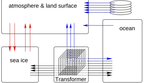
Figure 9 schematically illustrates possible communication pathways in a coupled application including the access of data from files. Depending on the respective grid configu-ration, the exchange of coupling data is handled in two dif-ferent ways. Data points that reside on identical geographical locations on the source and target side are exchanged directly between the component processes (involving repartitioning if necessary), without the participation of Transformer pro-cesses. Data points for which a regridding is required are sent through the Transformer. Matching and non-matching grid points are identified by the PSMILe solely based on the geographical description of the grid. In order to reduce the amount of messages to be exchanged, the current implemen-tation assumes that the number of matching points must at least sum up to 10% of the total number of grid points to be sent. For any number below this threshold, matching data are exchanged together with non-matching data through the Transformer processes.

The data transfers, either direct or through the Trans-former, are handled in parallel, in the sense that the source and grid point values corresponding to the different intersec-tion regridding lists (see Sect. 6) are transferred separately. Gathering or scattering is never performed, and all compo-nent processes that are active in the coupling participate in the exchange. One Transformer process may treat several intersection regriddings when the number of source and tar-get domain intersections exceeds the number of Transformer processes.

atmosphere & land surface

sea ice

Transformer

ocean

Fig. 9. Example of communication pathways in an OASIS4 coupled

application.

To further optimise the exchange of data and to reduce the work load of the Transformer processes, only non-masked source and target points are transferred. On the receiver side, the non-masked data are scattered onto the destination ar-ray behind the PRISM Get call and provided to the API in the appropriate array shape leaving masked target points un-touched. The calculation of regridding weights in the Trans-former is delayed until the first exchange for which a partic-ular set of weights is required. The weights are then stored in the Transformer for subsequent exchanges.

It is noteworthy to mention that the data are buffered in the PSMILe library on the sender side outside the MPI li-brary. Data are transferred with a so-called non-blocking MPI function (MPI Isend). With a standard conform MPI implementation, this guarantees no overflow in MPI internal buffers. The PRISM Put will immediately return when the data are stored locally even if the destination process (be it the Transformer or another component in case of direct com-munication) is not yet ready to receive data. On the sender side the user code outside the PSMILe can safely progress and reuse its own local memory. The PRISM Get on the other hand will only return when the data are received.

(13)

compliant with the pNetCDF library (Li et al., 2003). When linked against pNetCDF, data are written into and read from a single file via MPI-IO with no p or postprocessing re-quired. From a user perspective, this approach is invariant to changes in domain partitioning and should also provide a rea-sonable IO performance provided that the respective MPI-IO implementation efficiently uses the underlying system archi-tecture (memory layout and file system).

During the data exchange and IO, the PSMILe is able to invoke some local transformation routines like time-accumulation, time-averaging, gathering and scattering of physical fields. It performs the required transformation lo-cally on the source side before the exchange with other com-ponents of the coupled system or IO. In this case only the end product is communicated to the target.

8 Performance

Before seriously considering a new software for a coupled system a user typically asks for the cost of coupling and the overhead one has to consider for the coupling. Prefer-ably, a user would like to have exact numbers at hand in terms of CPU seconds or a percentage of time relative to an non-coupled system. For full ESMs, it is difficult to pre-dict the additional time needed for the coupling. To some degree, this depends on the search that has to be performed on a variety of grids for a larger number of exchange fields and different regriddings. Another important aspect is the run-time behaviour of the different ESM components and the load-(im)balancing between the processes involved. This may strongly influence the time needed to perform a data ex-change. ESMs differ from each other in the above mentioned aspects, and providing a number for a particular ESM is of little help and not in the scope of this article. In addition, the picture may again change completely when an ESM job is running in batch mode and eventually has to share some resource with competing applications. In the following, our aim is to give a first idea about the potential cost for coupling and to provide information about the efficiency of the cou-pling software as such. Therefore we try to exclude the afore-mentioned side effects as much as possible. We will revisit this subject in our discussion in Sect. 9. We now use a sim-plified test case application to demonstrate the performance of the OASIS4 search algorithm and the data exchange and compare them with OASIS3 performance.

8.1 Benchmark design

Here we investigate the so-called “strong scaling” properties of OASIS4. By keeping the global problem size constant, we expect a decrease in CPU time for individual processes with the problem distributed to larger number of processes in proportion to the local problem size. While this is in ge-neral reflecting the typical situation the user is confronted

with, strong scaling is considered more difficult to achieve (in contrast to weak scaling where the local problem size is kept constant and the global problem to be solved is in-creased with increasing numbers of processes used). The test case we are considering now is a bidirectional exchange of 2-dimensional data between a global “atmospheric” grid for component A and an “ocean” grid for component B, rang-ing from 0◦ to 360◦ in longitude and latitudes φ between 70◦S and 70◦N. Both grids are described as horizontally ir-regular grids in order to bypass the optimised routines that are available for completely regular grids and to mimic the large class of use cases, the 2-D data exchange between any two physical components at the Earth surface. Some of the ocean and atmosphere grid points have been masked out in order to bypass additional optimisation steps of the search al-gorithm which can be applied if complete non-masked grids are treated. The components are partitioned in latitude di-rection. The search is performed for bilinear interpolation without requesting an extra nearest-neighbour search for tar-get points that only have masked “bilinear” source points (see Sect. 5.1). The search is performed for one exchange field for each direction.

In Sect. 8.2, we consider a T255 “atmospheric” grid with 768×385 grid points for component A and an “ocean” grid with 0.3◦×cosφhorizontal resolution corresponding to 1202×665 grid points for component B. In an additional test described in Sect. 8.3, we have expanded the problem into the vertical dimension towards a full 3-D search and data exchange with 40 levels for component A and 45 levels for component B. In Sect. 8.4, the resolutions of component A and component B are increased respectively from T21 to T255 and from 4.0◦_×cos_φ_{to 0}_.₅◦_×cos_φ_.

8.2 2-D search and exchange

For this particular benchmark calculations and for the 3-D cases described in Sect. 8.3, the OASIS4 sources have been compiled with the Intel Fortran compiler version 10.1 and the GNU C compiler version 4.1.2, both using default com-piler switches without any further optimisation. The code has been run on a local PC cluster. Each node of the cluster is equipped with 2.0 GHz 2 times single core AMD Opteron processor 246 and 4 GB of memory per node connected via a 2 Gigabit Myrinet. For the message passing, we use the Mes-sage Passing Interface Chameleon Glenn’s MesMes-sages propri-etary communication layer (MPICH-GM) provided by Myri-com. For all tests, we have used the MPI1 method where all processes have to be started at once (see Sect. 3).

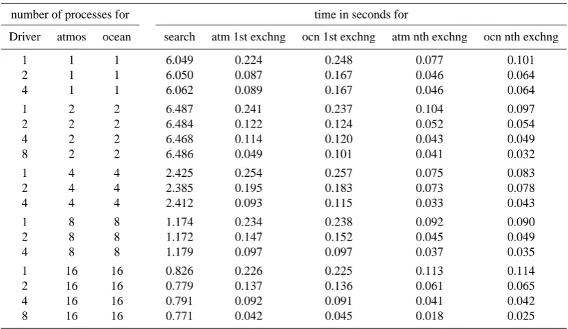
The numbers presented in Table 2 show the wall-clock time needed to perform the search for the bilinear inter-polation, the time needed to perform the first exchange of data (which includes the calculation of the weights for the bilinear interpolation in the Transformer), and the time needed for subsequent data exchanges (averaged over 100 data exchanges). When repeating the measurements the

(14)

Table 2. Performance of OASIS4 tasks obained on a PC cluster for 2-D search.

number of processes for time in seconds for

Driver atmos ocean search atm 1st exchng ocn 1st exchng atm nth exchng ocn nth exchng

1 1 1 6.049 0.224 0.248 0.077 0.101

2 1 1 6.050 0.087 0.167 0.046 0.064

4 1 1 6.062 0.089 0.167 0.046 0.064

1 2 2 6.487 0.241 0.237 0.104 0.097

2 2 2 6.484 0.122 0.124 0.052 0.054

4 2 2 6.468 0.114 0.120 0.043 0.049

8 2 2 6.486 0.049 0.101 0.041 0.032

1 4 4 2.425 0.254 0.257 0.075 0.083

2 4 4 2.385 0.195 0.183 0.073 0.078

4 4 4 2.412 0.093 0.115 0.033 0.043

1 8 8 1.174 0.234 0.238 0.092 0.090

2 8 8 1.172 0.147 0.152 0.045 0.049

4 8 8 1.179 0.097 0.097 0.037 0.035

1 16 16 0.826 0.226 0.225 0.113 0.114

2 16 16 0.779 0.137 0.136 0.061 0.065

4 16 16 0.791 0.092 0.091 0.041 0.042

8 16 16 0.771 0.042 0.045 0.018 0.025

differences in time are in the order of a few milliseconds. Therefore we decided not to include any statistics as this will not change the general picture we are going to discuss.

The time needed for the search can be represented by the time needed for the PRISM Enddef routine. The search is performed on the two sets of source component processes as the component A target points are searched for on the compo-nent B processes and vice versa. As the PRISM Enddef and subsequent calls therein contain blocking MPI calls, the total time needed by the PRISM Enddef is to a large extent con-trolled by the source process which has to solve the largest problem (mainly determined by the number of target points to be processed). The time spent in PRISM Enddef is almost identical for all processes due to this blocking nature of the MPI function calls used inside. Therefore only one number, the time needed by the component process with the largest data load is shown in the table for each setting.

In general, the wall clock time needed for the search de-creases with the number of processes dedicated to the com-ponents: in this case, the speed-up is roughly a factor of 8 when going from 2 to 16 processes. When going from one to two component processes, the time for the search is slightly increased. This can be attributed to the different algorithms used, as in the one-processor case certain subroutines do not have to be called simply because no boundary exchange is required on the source grid. When the number of processes is increased further the required wall-clock time is reduced significantly to values well below 1 s for the 2-D data ex-change on 16 processors. At this stage, the number of

Trans-former processes is not of critical importance as they are not involved in the search. Communication with the Transformer is established only when the search for an intersection sub-domain has been completed and search results are delivered to the Transformer process(es) (see Sect. 6).

(15)

We observe a general decrease of the wall-clock time for the exchange with an increasing number of Transformer pro-cesses available (Table 2). One reason is that the likelihood increases that the Transformer process is ready to receive, process and send data. The other reason is that the amount of data to be treated is reduced for each process. The only case when increasing the number of Transformer processes does not result in a decrease of the exchange wall-clock time is when the components themselves are not parallel and when the number of processes for the Transformer goes from 2 to 4. In this case, there are only two distinct intersection regrid-ding lists (see Sect. 6), i.e. one when considering one com-ponent as the source and another one when considering the other component as the source. As the different Transformer processes work in parallel over the regridding of the differ-ent source and target process intersections, the 2 additional processes (when going from 2 to 4 processes) do not get any workload and do not participate in the data exchange.

During the first exchange of data in addition to the process-ing of the exchange fields, the Transformer has to calculate the weights which are then stored and reused for subsequent data exchanges. This additional workload is responsible for the longer time needed to perform the first exchange when comparing with the time needed for subsequent exchanges.

We also observe that for a fixed number of Transformer processes the exchange time is fairly independent of the num-ber of application processes. As the data are exchanged through the Transformer processes, it can act as a bottleneck in the exchange if it is not sufficiently parallel. In general, it is the number of available Transformer processes that dic-tates the speed of the exchange and not the parallelisation of the components themselves.

Finally, we notice that the scaling behaviour is in general not fully predictable; this can mainly be attributed to the fact that a particular Transformer process may still be busy with other tasks, that data are sometimes not available from the source component or delivered only with a delay due to punc-tual load imbalancing. We observe super-scalability when going in our case from 2 to 4 processes for the components. In the 2-D case this super-scalability is also present when in-creasing the number of component processes further from 4 to 8 processes. Cache effects provide one possible explana-tion for this behaviour. A more efficient scheduling of the processes with a reduced waiting time for messages to arrive is another answer. A finer partitioning of the target grid may fit the remote partitioning better and thus reduce the overhead during the initial search.

8.3 3-D data exchange

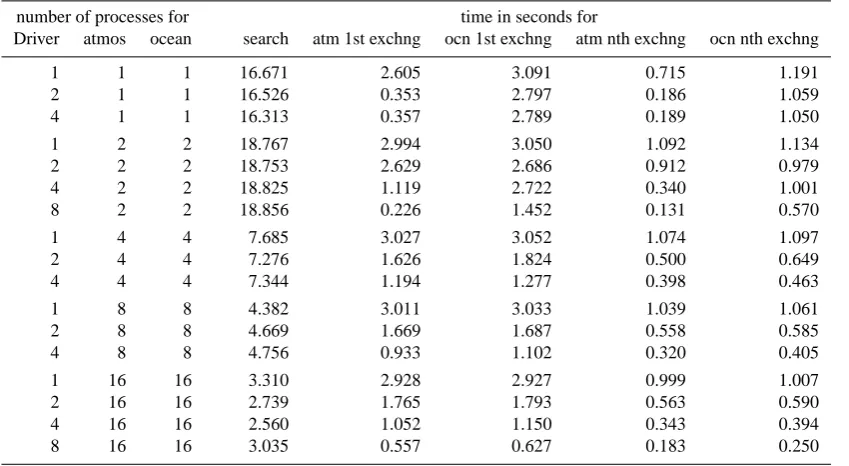
The general picture does not change much with an increas-ing amount of data to be exchanged, for example goincreas-ing from the 2-D to a 3-D coupling, i.e. when exchanging data be-tween 40 levels for component A and 45 levels for

compo-nent B (see Table 3). As in the 2-D case, the efficiency of the search mainly depends on the number of component pro-cesses available. The wall-clock time decreases by roughly a factor of 6 when going from 2 to 16 component processes. The time needed for the search decreases to only a few sec-onds when employing four or more application processes – which is likely the case with applications running with the grid sizes similar to our example. With an increasing num-ber of Transformer processes the exchange time is reduced as in the 2-D case.

8.4 Performance of the multi-grid search and parallel regirdding

To evaluate the performance of OASIS4 and in particular the efficiency of the multi-grid algorithm, the benchmark was adapted to the OASIS3 coupler and additional 2-D cou-pled runs were realized for different resolutions of com-ponents A and B. These additional runs were performed on a Single Core Intel Pentium 4 CPU 3.20 GHz Linux PC with MPICH-1 message passing. OASIS4, OASIS3 and the benchmark sources were compiled with the Portland Group Fortran Compiler 9.0-4 and with the GNU C compiler 4.4.1. One process was started for each component and the driver.

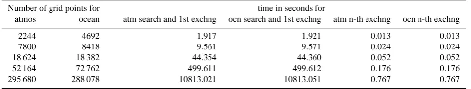
The results are presented in Table 4 for OASIS4 and in Table 5 for OASIS3. In each case, five runs were realized with a resolution ranging from T21 (2244 grid point) to T255 (295 680 grid points) for component A, and ranging from 4◦ (4692 grid points) to 0.5◦(288 078 grid points) for compo-nent B. In all cases, the Transformer and the compocompo-nents were running with one process each. The numbers provided in the tables give the time for the search and the 1st exchange as measured in component A (3rd column) and in component B (4th column). We provide these measures to have a compa-rable basis: with OASIS3, the neighborhood search and the weight calculation is done during the 1st exchange, where as they are respectively done during the initialisation phase below the PRISM Enddef call and during the 1st exchange with OASIS4. In addition, Tables 4 and 5 show the time for the n-th exchange in component A (5rd column) and in component B (6th column).

By comparing Table 4 and Table 5, we see that even at rel-atively low resolution (2244 and 4692 grid points for com-ponents A and B, respectively) OASIS3 is about two times slower than OASIS4. The difference gets bigger with in-creasing resolution: the time required for the neighborhood search and the first exchange (including the weights calcula-tion) increases with O(N) for OASIS4 (see Fig. 10) and with O(N2) for OASIS3. Even the time for subsequent exchanges is always about 50% higher with OASIS3 than with OASIS4. These numbers clearly demonstrate the benefit of the multi-grid neighborhood search when compared to a classi-cal search and the increased general performance of OASIS4 over OASIS3 even in this simple non-parallel case.

(16)

Table 3. As in Table 2 but for 3-D search and exchange.

number of processes for time in seconds for

Driver atmos ocean search atm 1st exchng ocn 1st exchng atm nth exchng ocn nth exchng

1 1 1 16.671 2.605 3.091 0.715 1.191

2 1 1 16.526 0.353 2.797 0.186 1.059

4 1 1 16.313 0.357 2.789 0.189 1.050

1 2 2 18.767 2.994 3.050 1.092 1.134

2 2 2 18.753 2.629 2.686 0.912 0.979

4 2 2 18.825 1.119 2.722 0.340 1.001

8 2 2 18.856 0.226 1.452 0.131 0.570

1 4 4 7.685 3.027 3.052 1.074 1.097