Earth Syst. Sci. Data, 2, 35–49, 2010 www.earth-syst-sci-data.net/2/35/2010/
©Author(s) 2010. This work is distributed under the Creative Commons Attribution 3.0 License.
History
ofGeo- and Space
Sciences
Open
Access
Advances
inScience & Research
Open Access Proceedings
Drinking Water
Engineering
and Science
Open
Access
Open
Access
Earth System
Science
Data
Drinking Water
Engineering
and Science
Open
Access
D
iscussions
Open
Access
Earth System
Science
Data
D
iscussions
Quality control procedures and methods
of the CARINA database
T. Tanhua1, S. van Heuven2, R. M. Key3, A. Velo4, A. Olsen5, and C. Schirnick1
1Leibniz-Institut f¨ur Meereswissenschaften, Marine Biogeochemie, Kiel, Germany
2Department of Ocean Ecosystems, University of Groningen, Groningen, The Netherlands
3Atmospheric and Oceanic Sciences Program, Princeton University, Princeton, NJ 08544, USA
4Instituto de Investigaciones Marinas – CSIC, Eduardo Cabello 6, 36208 Vigo, Spain
5Bjerknes Centre for Climate Research, UNIFOB AS, All´egaten 55, 5007 Bergen, Norway
and Department of Chemistry, University of Gothenburg, 41296 G¨oteborg, Sweden
Received: 18 June 2009 – Published in Earth Syst. Sci. Data Discuss.: 20 August 2009 Revised: 20 January 2010 – Accepted: 1 February 2010 – Published: 4 February 2010
Abstract. Data on the carbon and carbon relevant hydrographic and hydrochemical parameters from
previ-ously not publicly available cruises in the Arctic, Atlantic and Southern Ocean have been retrieved and merged to a new data base: CARINA (CARbon IN the Atlantic). These data have gone through rigorous quality con-trol (QC) procedures to assure the highest possible quality and consistency. All CARINA data were subject to primary QC; a process in which data are studied in order to identify outliers and obvious errors. Additionally, secondary QC was performed for several of the measured parameters in the CARINA data base. Secondary QC
is a process in which the data are objectively studied in order to quantify systematic differences in the reported
values. This process involved crossover analysis, and as a second step the offsets derived from the crossover
analysis were used to calculate corrections of the parameters measured on individual cruises using least square models. Significant biases found in the data have been corrected in the data products, i.e. three merged data files containing measured, calculated and interpolated data for each of the three regions (i.e. Arctic Mediter-ranean Seas, Atlantic, and Southern Ocean). Here we report on the technical details of the quality control and on tools that have been developed and used during the project, including procedures for crossover analysis and least square models. Furthermore, an interactive website for uploading of results, plots, comments etc. was developed and was of critical importance for the success of the project, this is also described here.
Data coverage and parameter measured
Repository-References:
doi:10.3334/CDIAC/otg.CARINA.ATL.V1.0
doi:10.3334/CDIAC/otg.CARINA.AMS.V1.2
doi:10.3334/CDIAC/otg.CARINA.SO.V1.0
Available at:
http://cdiac.ornl.gov/oceans/CARINA/Carina inv.html
Location Name: Atlantic Ocean, Southern Ocean, Arctic Mediterranean Seas
Correspondence to: T. Tanhua
1 Introduction
CARINA is a database of carbon and carbon-relevant data from hydrographic cruises in the Arctic Mediterranean Seas, Atlantic, and Southern Ocean. The project started as an es-sentially informal, unfunded project in Delmenhorst,
Ger-many, in 1999 during the workshop on “CO2 in the North
Atlantic”, with the main goal to create a uniformly formatted database of carbon relevant variables in the ocean to be used for accurate assessments of oceanic carbon inventories and uptake rates. The collection of data and the quality control of the data have been a main focus of the CARINA project. Both primary and secondary QC of the data has been per-formed. Experience with the previous GLODAP synthesis project (Key et al., 2004) demonstrated that a consistent data
product can be produced containing data from many diff
But it is essential that the results obtained by the different methods of quality control are compared and systematically assessed. This assessment is required largely due to the fact that standards do not exist for many oceanographic measure-ments. Since CARINA included a large number of scien-tists from all over the world, communication of individual
efforts and results were important. For this purpose, the
dividual data analysts and the working groups used an in-ternet based platform for posting their results, including
up-loading/downloading and viewing of figures, data and
com-ments. In this way, the data analysts were sharing experience and results in real time. In addition to the interaction over the web portal and email communication, 3 workshops were held where practical matters and the adjustments of data were discussed, and finalized. This report provides an overview of the methods and techniques used for the quality control of the database. A more comprehensive description of the com-plete CARINA database can be found in Key et al. (2009) as well as in other papers in this special issue.
2 Data provenance
The CARINA database includes data and metadata from 188 oceanographic cruises or projects, i.e. entries to the cruise
summary table (http://cdiac.esd.ornl.gov/oceans/CARINA/
Carina table.html). A few of the cruises listed in the ta-ble are collections of several cruises or time series stations. In addition, 52 reference cruises are included in the sec-ondary QC to ensure consistency with historical data (i.e.,
WOCE/GLODAP). These reference cruises are not included
in the CARINA data base, but on several occasions are
sug-gestions for adjustments made that are different from those
applied to the GLODAP data base. Due to the volume of the data set, the CARINA data are divided in three regions: Arc-tic Mediterranean Seas (AMS); AtlanArc-tic Ocean (ATL), and Southern Ocean (SO), each of them with a working group that carried out the secondary QC. A few of the CARINA cruises are common to the ATL and SO groups, and a few cruises are common to the ATL and AMS groups. In these cases there has been agreement between the groups on all adjustments. This provides a consistency control in the sec-ondary QC between the CARINA working groups.
The CARINA database consists of two parts: the first part is the individual cruise files where all the data reported by the measurement teams are stored. Quality flags are accom-panying the data. In many cases the flags are those originally reported, in others cases the flags were assigned by R. Key. These files are in WHP (WOCE Hydrographic Program)
ex-change format (http://whpo.ucsd.edu/format.html). The first
lines of each file are the condensed metadata. There are no calculated or interpolated values in the individual cruise files, except for pressure calculated from depth. No adjustments have been applied to any of these values with the excep-tion that all pH measurements were converted to the
sea-water pH scale at 25◦C. Recently, the international ocean
carbon measurement community decided that new pH mea-surements would be reported on the total hydrogen scale, but that decision occurred too late to be incorporated into this project.
The second part of CARINA consists of three merged data files; one each for the Atlantic Ocean, Arctic Mediterranean Seas and Southern Ocean regions. These files contain all the CARINA data judged to be “good”, and also include: 1) in-terpolated values for nutrients, oxygen and salinity if those data were missing and the interpolation could be made ac-cording to certain criteria, as described in Key et al. (2009); and 2) calculated carbon parameters; e.g. if Total Carbon
Dioxide (TCO2) and Total Alkalinity (TA) were measured,
pH was calculated, 3) instances where bottle salinity was missing or bad were replaced with CTD salinity, if possi-ble. Values for any of these cases have been given the quality flag “0”. In many cases there are additional parameters in the individual cruise files which have not been included in the
secondary QC, such as∆14C,δ13C and SF6. Some of these
are included in the merged data files as well.
A significant and time consuming part of the CARINA synthesis was the data collection, merging of subsets of data from individual cruises and conversion of units to a
com-mon format/standard, see Key et al. (2009). The next step
in the synthesis was the quality control (QC). Our quality control procedures are comprised of two distinct steps. First the reported measurements are studied in order to identify outliers and obvious errors, i.e. primary QC. Secondly, we
quantify systematic differences in the reported values in a
process called secondary QC. Essentially, primary QC is a check of precision and secondary QC is a check of accuracy. These QC processes were performed on the data sets reported by the measurements teams, and are distinct from the qual-ity assurance (QA) procedures originally performed by each
cruise measurement team in order to ensure sufficient quality,
which is part of the data collection and analysis procedures. A flowchart of the procedures involved in the process of pro-ducing the CARINA data product is presented in Fig. 1.
3 Primary quality control
for each cruise
for each region acquire original data
contact PI about outliers
flag data
store individual cruise file
submit cruise files to CCHDO
submit dataproducts to CDIAC scan data for outliers
calculate carbon parameters interpolate missing values add reference cruises
split data into 3 regions
assess inversion results
decide on adjustments
apply adjustments
merge adjusted cruises
store dataproduct remove reference cruises store results on web platform
determine offsets between cruises
convert to standard units
remove not-good data start
QC1
QC2
perform inversion assess offsets
Figure 1.Flowchart describing the principal steps during the sec-ondary quality control; see text for details.
Table 1.Table listing the flags used for the CARINA cruises. Only flags 0, 2 and 9 are used for the data product. Flag 0, approximated, refers to interpolated values for nutrients, oxygen and salinity, and to calculated carbon parameters, see text.
Flag Value Interpretation in CARINA
0 Approximated
1 Not used
2 Good
3 Questionable
4 Clearly bad result
5 Value not reported
6 Average of replicate
7 Not used
8 Not used
9 Not measured
to flagging each datum with an integer. Nine different flag
values were defined (0–9, see Table 1 for definitions). This system, which has been continued in subsequent major ocean sampling programs and was used for the GLODAP data syn-thesis, was adopted for CARINA. It is important to note that data flagging or primary quality control deals only with data precision. The techniques used to assign these flags are usu-ally insensitive to data bias particularly in cases where all of the measurements of any parameter for a cruise are biased relative to results from other cruises.
A large number of the CARINA cruises predate the cus-tom of data flagging. Consequently, as the raw data files were accumulated, flags were initialized with flag value 2 (good) for each measured variable (except temperature) or 9 (not measured) when there was no measured value. Subse-quently, the various measured parameters were analyzed with the same software and techniques used for modern cruises. Essentially, various property-property plots are examined for small groupings of stations looking for outliers. Notes were kept for each outlier in each plot. Measurements that were outliers, generally in more than one type plot, were flagged
questionable (3) or bad (4) with the difference between these
two flags being one of degree. Whenever possible, the data
values flagged 3/4 were reported back to the person
origi-nally responsible for the measurements for confirmation. In cases of disagreement, the choice of the data generator was used. In general whenever a datum was borderline between good and questionable, the good flag was retained. Addition-ally, during the flagging significantly more variability was al-lowed for points that were in the upper thermocline or near-bottom. Near-surface values were virtually never flagged
3/4 with the only exception being totally unrealistic values
and/or obvious clerical errors.
This method of data flagging is quite subjective regard-less of who assigns the flags. With very few exceptions all of the CARINA cruises were flagged at Princeton (R. Key). This does not mean that the flags were assigned correctly, but does ensure that the assignment was done as consis-tently as possible and additionally that the flags were con-sistent with those assigned to the carbon parameters during preparation of GLODAP (Key et al., 2004). The only flags not assigned at Princeton were associated either with very recent cruises (generally WOCE or CLIVAR) or with data streams from labs which had participated in WOCE and as-signed flags to their own data routinely (mostly CFC data
from M. Rhein and/or R. Steinfeldt). Whenever data were
submitted with flags, the flag values were simply checked
for obvious/clerical errors. The CARINA data product
incor-porates one additional flag with value zero (0). This flag was also used in GLODAP. The zero flag indicates a datum that “could have been measured”, but was approximated in some
manner. There are three different uses for the zero flag in the
data products: 1) Instances where bottle salinity was missing or bad and consequently replaced with CTD salinity, 2) in-terpolated values for salinity, oxygen or nutrients, or 3) for calculated carbon parameters.
The secondary quality control procedures used here (dis-cussed below) critically examine the data using techniques
quite different from the routine primary QC methods. In
4 Secondary quality control
Secondary quality control is a process in which the data are objectively studied in order to quantify systematic biases in the reported values. The identified data biases are then sub-jectively compared to predetermined accuracy limits. Spe-cial consideration is given to the fact that some of the regions studied are known to have had real temporal change over the time period covered by the various cruises (1977–2007). Ob-viously, one does not want secondary QC to “erase” real tem-poral change. The nature of the secondary QC procedure is
such that various data recording errors/outliers are also
iden-tified in the process, thus complementing the initial primary QC. Data from cruises that show significant bias are given an adjustment (either multiplicative or additive), that is ap-plied to the data product (i.e. the merged data files for the three regions), but not to the individual cruise files (those remain as reported with measured data). Data with lower than acceptable quality are also identified; questionable data are removed from the data product, but retained in the in-dividual cruise files with appropriate flags. The parameters considered in the secondary QC are salinity (and in a few cases CTD salinity), oxygen, nitrate, phosphate, silicate, al-kalinity, total inorganic carbon (DIC), pH, CFC-11, CFC-12,
CFC-113 and CCl4.
The most important tool in the secondary quality control of the CARINA data was the crossover analysis. Other ap-proaches that were used include multiple linear regression (MLR) analysis and relation between measured parameters, such as CFC-11 vs. CFC-12. This report focuses on the crossover analysis and the least square models (inversions)
that followed to determine the corrections/correction factors
needed to minimize the offsets between cruises.
4.1 Crossover analysis
Crossover analysis is an objective comparison of deep wa-ter data from one cruise with data from other cruises in the same area. Crossover analysis has been performed earlier on, for instance, the WOCE and JGOFS data set (e.g. Sabine et al., 1999; Gouretski and Jancke, 2001; Johnson et al.,
2001; Sabine et al., 2005), see also http://cdiac.esd.ornl.gov/
oceans/glodap/crossover.html, where the concept was laid
out. These results have increased the internal consistency of, for instance, the GLODAP data set. In CARINA we have used the basic concept of crossover analysis.
The result of a crossover analysis is an offset. Offsets are
defined as the difference between two cruises, A and B,
de-rived from a crossover analysis. If the offset for cruise A
(relative to cruise B) is less than zero (or unity, for multi-plicative parameters), then cruise A data would have to be increased in order to be consistent with cruise B (or vice
versa). The offset were quantified as multiplicative factors
for nutrients, oxygen and CFCs, and as additive constants for salinity, DIC, and alkalinity. There are several reasons
for this division between additive and multiplicative offsets.
Firstly, multiplicative offsets eliminate the problem of
poten-tially negative values for any variable with measured concen-tration close to zero, i.e. in the surface water for nutrients, or oxygen concentrations in low oxygen areas. Also, for nu-trients and oxygen analysis, problems in standardization are
the most likely source of error, hence a multiplicative offset
is deemed as appropriate. For DIC, alkalinity and salinity an additive adjustment seemed most likely, due to, for instance, biases in the reference material used. Similarly, since pH is
a logarithmic unit, only additive offsets can be considered.
In the crossover analysis, clustering or cluster analyses was often performed. This refers to a subroutine in the crossover analysis for cruises that fall in more than one region, or for crossovers that cover such a large and diverse area that the crossover is divided into more “sub-crossovers”, i.e. clusters. When we discuss crossover analysis in the following, clus-tering is included, i.e. the crossover analysis between two cruises takes the geographic distribution of the cruises into consideration, either manually or automatically. The station distribution in CARINA was such that the definition of “same area” was variable and defined subjectively on a case by case basis, but the compared stations were normally within 2
de-grees of latitude, i.e.∼222 km. Mostly, the two cruise tracks
are crossing each other; hence the name “crossover
analy-sis”, but it can also be repeat or parallel cruise tracks, which
is often the case for the CARINA data. We identified and analyzed more than 2100 individual crossovers for the CA-RINA data set.
Since the upper water column is more sensitive to variabil-ity on various time-scales than the deep ocean, only the deep part of the water column was considered for the analysis. For the ATL and SO regions, this minimum depth (i.e. pressure) was 1500 dbar. However, due to the deep mixed layers some-times found in the AMS region, the minimum depth was set to 1900 dbar for the Nordic Seas region as this is deeper than the ventilation depths observed over the time span covered by CARINA (Ronski and Budeus, 2005). The crossover analy-sis was performed on either pressure, density (i.e., sigma-4), or potential temperature surfaces. To account for vertical shifts of properties (i.e., internal waves etc.), the crossover analysis are normally done on density surfaces. However, in the Nordic Seas crossover analysis was made on depth sur-faces due to the small density gradients there. Arguments for the use of theta over sigma include the superior mea-surement accuracy of temperature and its independence of other parameters (especially biases in salinity are impossi-ble to clarify in sigma-space, since sigma itself is a function of salinity). One of the collections of software-routines that
were developed for the CARINA effort determined offsets in
each of the three spaces simultaneously, and its results allow
for comparison. The quality of the determinations of offsets,
most cases however, there were only small differences in the
offsets calculated in the three different ways, which gives us
some confidence in the analysis, see below.
As a first step in the crossover analysis, the profiles of the parameter in question for all stations included in a crossover were interpolated with a Piecewise Cubic Hermite Interpo-lating scheme. An important feature of this algorithm is that interpolated values almost never exceed the range spanned by the data points. That is, the Hermitian function has low tendency to “ring”. Large vertical gaps in the data were not interpolated, the definition of “large” being depth-dependent; larger “gaps” were allowed in the deeper part of the profile. In the case of density, the profiles were interpolated in such a way that the interpolated values were roughly equally dis-tributed in depth space. Practically this was done by letting a density profile that was typical for the area determine the in-terpolation distances in density space. This was done in order
to have sufficient weight (or “interpolated data points”) in the
deep water column were the properties of the water are sup-posed to change only slowly, and were the density gradients are often small.
Essentially, we distinguish between three routines for the crossover analyses carried out during the CARINA project: the manual crossover routine, and the two automatic rou-tines; running-cluster and cnaX-scripts, see below. These codes and routines developed during the project, so that man-ual crossover results obtained in the early part of the project are not necessarily made with the same assumptions as those made in the later part of the project. This applies also for the automated routines, but in this case the full data set was analyzed again when new routines were developed.
How-ever, even if the codes are slightly different, the results were
mostly very similar, as we will see below.
Due to the large number of crossovers in CARINA, the task of manually generating crossovers and entering the re-sults in an online table soon become overwhelming in terms of workload. Even though the process of manually gen-erating the crossovers lead to quality checked results, the process of manually entering the values in a table is prone to typos and errors that might bias the results of the inver-sions. Even though the automatically generated crossovers were, in general, used for the inversions, the manually gen-erated crossovers were invaluable as reference points in the decision process for suggesting adjustments. The matlab routines used for the secondary QC of CARINA, as well as all figures generated during the secondary QC can be
viewed and downloaded from http://cdiac.ornl.gov/oceans/
CARINA/Carina inv.html.
4.1.1 Manually generated crossovers
For the manually performed crossovers, an average profile (and its standard deviation) was calculated using all stations in each cruise that were closer to any station of the other cruise than the minimum horizontal distance. For this
av-eraging process, the interpolated profiles were used. These two average profiles were then compared to each other in a
second step, and the weighted offset and standard deviation
of the crossover were calculated. The disadvantage of this method is that the crossover can cover large area with
po-tentially very different hydrography, for instance for repeat
cruise tracks, and the offset for the crossover might thus be
biased. In this case, groups of stations for each cruise within a hydrographical regime were sought, and a crossover was divided into several sub-crossovers, “clusters”. The analyst then had the choice of using the average of all clusters to
cal-culate the crossover offset, or to discard clusters in areas of
known high variability, such as just south of the Greenland-Scotland ridge. The analyst then entered the results from the crossover analysis to the CARINA website, and uploaded the figure for the crossover.
4.1.2 The “Running cluster“-crossover routine
The crossover version called “running-cluster” was mainly used for automatically generated crossovers. In this routine the interpolated profile from each station in cruise A was compared to each interpolated profile from all cruise B sta-tions within the maximum distance for a valid crossover, and
a difference profile was calculated for each such pair. This
process was repeated for each station in cruise A which nor-mally results in several, up to hundreds for a repeat section,
difference profiles. The crossover offset and its standard
de-viation was calculated as the weighted mean and standard
deviation of the difference profiles of each crossover pair,
i.e. the part of the profile with low variability weigh higher in the calculation (often, but not always, the deeper part of the profile). This way of performing the crossover analysis has the advantage that only individual stations within the mini-mum horizontal distance are compared to each other. Hence,
even for repeat cruises covering several different
oceano-graphic regimes, the offset between these cruises can be
calculated in a straight forward manner. An example of a crossover is shown in Fig. 2.
4.1.3 cnaX crossover routine
This routine is essentially a fully automated implementation of the manual approach described above. Please note that, for the sake of readability, these paragraphs deal only with
the determination of offsets in depth-space, but the software
concurrently calculates offset profiles in density and
Figure 2. An example of a typical crossover made for oxygen in the eastern North Atlantic made by the running-cluster routine.
full run from raw-data loading to output of a final set of rec-ommendation for cruise parameter adjustments takes about 8 h on a regular computer for the complete CARINA data set. This includes the production of several tens of thousands fig-ures and dozens of tables, useful for tracing the script’s steps to determine problem areas. At the highest level of user in-teraction, each of the steps concerning clustering and quality assessment require user input; a full run may take up to sev-eral days to complete this way. This method gensev-erally results in a somewhat reduced amount of uncertainty in the final
out-put since badly determined offsets that may slip through the
automatic quality check can be caught by the user manual interaction. A flowchart describing the various steps in the crossover routines is presented in Fig. 3 to help guide the reader.
In either form, the routine first loads all individual cruise data. During this step the user is allowed to specify
subdi-vision of certain cruises if sufficient reason exists to assume
changes in instrument calibration during, for instance, port calls or instrument changes. Maps showing cruise-track, sta-tion locasta-tions and bathymetry are created for each cruise for possible user inspection. After this a crude scan is made to check which cruises share a geographical area, and therefore
may cross each other. During a subsequent refining step these potential matches are more closely analyzed. Stations are only considered for possible relevance for crossover analy-sis when certain criteria for parameter availability, minimum sample depth and number of samples are met. This approach saves considerable time over a full station-vs.-station prox-imity check.
Knowing which cruises can be compared with which other, i.e. cruise-pairs; a clustering method is employed to group stations from cruise A in close proximity to stations of cruise B into distinct geographical clusters. This clustering is either user-controlled, allowing the analyst to specify fur-ther clusters, reduced clustering or discard clusters, or fully automatic mode in which stations are progressively further clustered until the spatial dimensions of each cluster meet pre-set criteria. Limits also apply to the minimum num-ber of stations per cluster that should be retained. The re-sults of the clustering operations are stored in tabular form as well as drawn on maps. After all cruise-pairs have had their
“crossover stations” geographically clustered, offsets are
de-termined for each parameter for each cluster. As a first step the profiles are interpolated to about 75 levels in the range be-tween 2000 m to the deepest sample of either of the cruises.
Offsets are determined and expressed both as additive off
-sets and multiplicative offsets taking considerations outlined
above into account. These calculations closely follow the procedure outlined by Johnson et al. (2001).
After this “discrete clusters”-method of determining off
-sets, a “running cluster” approach is taken (as detailed above and comparable to the “running cluster”-routines) for
an-other determination of offsets. For cruise-pairs in which
both cruises have several dozens of stations in close prox-imity to stations of the other cruise (e.g. repeat lines) the running cluster routine potentially results in several hundred station-pairs. Of these only the 100 most closely spaced
station-pairs are further considered. The measurements at
each of these stations are interpolated to∼75 depth levels.
For each station-pair the offset profile is determined by
sub-traction/division of B’s interpolated profile from/by A’s. The
offset profiles are subsequently averaged to get the mean off
-set profile (MOP) and an associated offset standard deviation profile (OSDP) for this cruise-pair. The interpolated values
in the MOP are averaged and weighted by the OSDP,
result-ing in a weighted mean offset (WMO) for this cruise-pair.
The uncertainty of the value thus determined is expressed
by the associated weighted mean offset standard deviation
(WMOSD). It is these last two values that are used as in-put for the inversion. As mentioned above, the routine con-currently determines WMO and WMOSD in depth-, theta-and sigma4-space. The determined WMO with the smallest associated WMOSD (generally the one in sigma4-space), is
considered to be the best estimate of the cruise-pair’s offset.
The overall quality of the offset determined this way is
as-sessed through the use of several conditional statements
for all cruisepairs
for all parameters
for depth, σ4, θ
start
proceed to inversion
load station data of all cruises setup run (define thresholds, limits, clustering method, etc.)
find cruisepairs (i.e., pairs of cruises in same region)
which method?
running cluster discrete cluster
find up to 100 closely spaced stationpairs
which parameter?
subdivide the sta-tions into clusters
load measurements
interpolate profiles
calculate all offset profiles (A-B)
between SPs
calculate all ratio profiles (A/B)
between SPs
calculate weighted mean ratio
and S.D. calculate weighted
mean offset and S.D.
store results draw figure
do results appear to be reliable?
for all stationpairs S, AT, CT
yes no
O2, NO3
PO4, Si
load measurements
interpolate profiles
store results
store metadata of cruisepair
do results appear to be reliable?
for all cruisepairs
for all parameters
for depth, σ4, θ
yes no
calculate mean profile of each cruise
which parameter?
calculate offset
profile (A-B) calculate ratioprofile A/B
calculate weighted mean ratio and
statistics calculate weighted
mean offset and statistics
draw figure
S, AT, CT
O2, NO3 PO4, Si
for all clusters
discard results discard
results
average the results of the individual clusters store metadata
of cruisepair
Figure 3.Flowchart describing the steps involved in the cnaX crossover routines.
and the OSDP. Alternatively, the user can manually rate the
quality of the determined offset. This quality assessment and
the WMOSD are later used in the inversion for weighing
the offsets. The running-cluster-routine was determined to
yield superior results to the discrete-cluster-routine as it of-fers more rapid processing and is more objective. The results of the cnaX routines were made available to the analysts on the website and used for determination of adjustments.
4.2 Inversions
A second step in the secondary QC uses the offsets and
stan-dard deviations derived from the crossover analysis to cal-culate corrections of the parameters measured on individual cruises using least square models (Wunsch, 1996), i.e. in-versions, following the methodology described in Johnson et al. (2001). The inversion produces a correction factor (for
multiplicative corrections) or a correction (for additive cor-rections) for each of the cruises in the analysis. Indiscrim-inate application of these factors might produce the most uniform data set, but this would also remove real temporal
trends, an undesirable side effect. Therefore the corrections
and correction factors were manually evaluated; those that were actually applied to the data product are called
adjust-ments, to avoid confusion with the corrections suggested by
the inversion process.
Johnson et al. (2001) presented three models of different
Table 2. Table listing: (2nd column) the minimum adjustment applied to the data product; (3rd and 4th columns) the maximum model error in the Weighted Damped Least Square (WDLSQ) in-versions for core cruises and non-core cruises; (5th column) the
RMSE of the difference in offsets calculated by the running-cluster
and the cnaX routines.
Model error
Parameter Minimum Core Non-core cnaX-RC
adjustment cruies cruises
Salinity [ppm] 5 5 30 7.7
TCO2[µmol kg−1] 4 4 15 3.6
TAlk [µmol kg−1] 6 6 20 2.9
pH 0.005 0.005 0.010 NA
Nitrate [%] 2 2 20 2.9
Phosphate [%] 2 2 20 4.2
Silicate [%] 2 2 20 7.0
Oxygen [%] 1 1 10 1.1
the quality of the measurements. In the slightly more com-plex model, Weighted Damped Least Square (WDLSQ), a priori assumptions on the quality of the data are made; es-sentially the maximum allowed range of adjustments is set for each cruise, the model error. As Johnson et al. (2001) point out; this limitation tends to decrease the adjustments of individual cruises on cost of the overall performance of the model. Finally, the simplest of the models, Simple Least
Squares (SLSQ), do not take the uncertainty of the offset
val-ues into account, and is considered too simple.
For instance, both the work of Johnson et al. (2001) and Lamb et al. (2002) dealt with a set of cruises with presumable similar quality since they all aimed at meeting the WOCE Hydrographic Program (WHP) standards. The CARINA data base, in contrast, is a collection of cruises that covers more
than 2 decades with different scope and standards of the
measurements. The quality of the measurements is more heterogeneous for CARINA than for the WOCE data set. Therefore, the CARINA group performed both WLSQ and WDLSQ inversions of the crossover results, and the results from both were considered in determining the adjustment of a cruise. Since there is such a heterogeneity among the CA-RINA data, for the North Atlantic and Southern Ocean areas, a number of core cruises were identified, see above, where the quality of the data were, in general, assumed to follow WHP targets. The core cruises thus includes the reference
cruises (i.e. WOCE/GLODAP cruises) for the SO area; for
the NA area a number of non-reference cruises were addi-tionally included as core-cruises (Tanhua et al., 2009). These core cruises were generally given low model error for the WDLSQ analysis whereas the non-core cruises were given high model errors, i.e. the corrections of the non-core cruises were allowed to be larger than those for the core cruises,
Table 2. In this way, the model tended to adjust the CA-RINA dataset towards the values of the core-cruises. In most
cases, however, there were only small differences between
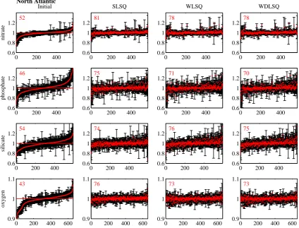
the WLSQ and WDLSQ inversions. As the CARINA project didn’t blindly follow the inversion results we used both the WLSQ and WDLSQ models for the analysis; see Fig. 4 for an example of the result of an inversion for the multiplicative parameters for the CARINA-ATL data set.
There are some important additions/alterations to the
in-version methods used in CARINA compared to Johnson et al. (2001). Firstly, since the time-span over which the hy-drographic surveys took place is large (up to 3 decades) and trends in deep water properties can be expected on this time frame over large parts of the CARINA domain, a time
fac-tor, KT, was weighted into the inversions. This factor was
calculated as unity plus the time in years between the two cruises in a crossover times 0.1, i.e. KT=1+∆year×0.1, and
multiplied to the standard deviation of a crossover. This re-duces the impact of a crossover on the inversion if the time elapsed between the two cruises is large. One can argue that the time factor should be larger for more active parts of the ocean, for instance the Labrador Sea, than in “calmer” parts of the Ocean, such as the subtropical eastern Atlantic. How-ever, since such classification tends to be rather arbitrary and
difficult to implement, no such area dependent weighting was
conducted for CARINA. This was rather done manually by the analyst in the final determination of the adjustment. That is, data from a “variable” area were generally allowed larger
offsets (i.e. higher suggested corrections from the inversion)
than data from a “quiet” area of the ocean before an adjust-ment was accepted.
4.3 Determination of adjustments
Many potential sources of uncertainty can complicate an oth-erwise straightforward assessment of cruise biases. Exam-ples include: 1) temporal variability and long-time trends in parameter values on a particular location in the ocean, 2) drifting or variable measurement precision and accuracy during a cruise, 3) profile interpolation errors, and 4)
dif-ferences between routines used to determine offsets. Since
biases cannot be determined with absolute accuracy, the CA-RINA working group agreed to correct only biases greater than a certain threshold value, Table 2. These thresholds re-flect the expected minimum bias that should be possible to determine with reasonably certainty. For highly variable re-gions or for cruises with few deep data points, larger uncer-tainty was allowed in the manual evaluation of corrections.
Aided by the corrections suggested by the inversions and
the offsets of all crossovers for a cruise/parameter
combina-tion, the potential bias for each cruise and parameter was scrutinized by the analyst. Particular emphasis was put on crossovers with core cruises and from crossovers with good
statistics (i.e. larger number of stations/samples) in “quiet”
0 200 400 0.6
0.8 1 1.2
Initial
52
nitrate
North Atlantic
0 200 400 0.6
0.8 1 1.2
SLSQ
81
0 200 400 0.6
0.8 1 1.2
WLSQ
78
0 200 400 0.6
0.8 1 1.2
WDLSQ
78
0 200 400 0.6
0.8 1 1.2 46
phosphate
0 200 400 0.6
0.8 1 1.2 75
0 200 400 0.6
0.8 1 1.2 71
0 200 400 0.6
0.8 1 1.2 70
0 200 400 0.6
0.8 1 1.2 54
silicate
0 200 400 0.6
0.8 1 1.2 74
0 200 400 0.6
0.8 1 1.2 76
0 200 400 0.6
0.8 1 1.2 75
0 200 400 600 0.9
1 1.1
43
oxygen
0 200 400 600 0.9
1 1.1
76
0 200 400 600 0.9
1 1.1
73
0 200 400 600 0.9
1 1.1
73
Figure 4. The results of an inversion of the North Atlantic nutrient and oxygen data: Left column (initial) shows the offsets of all the
crossovers sorted by offset (red dots) and the weighted standard deviation of the crossover (black bars); the following columns shows the
offsets after the corrections suggested by the SLSQ, WLSQ and WDLSQ inversions has been applied to the data. The numbers in the panels
indicate the percentage of crossovers that are indistinguishable from zero within their uncertainties.
additional evidence was considered by the analyst, such as
the relation to another parameter (e.g. nitrate/phosphate or
CFC11/CFC12 ratios) and whether or not certified reference
material (CRM) was used. Finally, an adjustment was sug-gested by the analyst and entered into the online adjustment table. Only significant adjustments were applied, generally
rounded to the nearest full percent, µmol/kg or ppm (for
salinity). This somewhat subjective process makes the
CA-RINA project different from most previously published
con-sistency analyses of hydrographic data. The subjectivity pos-sibly makes CARINA more prone to errors made by the an-alyst, but at the same time makes the CARINA adjusted data potentially more robust. In case of doubt, the CARINA team always tried to err of the side of not making an adjustment. The CARINA adjustment decision mechanism was similar to GLODAP, but the CARINA mechanics used to quantify the adjustment were much more sophisticated than those of GLODAP.
The lines of evidence for an adjustment (or the
ab-sence thereof) can be found at http://cdiac.ornl.gov/oceans/
CARINA/CARINA QC.html in the form of comments and
relevant figures, see Sect. 6. These adjustments were vetted during the final CARINA workshop in Paris in June 2008. Additionally, a second crossover analysis and inversion was made using the adjusted CARINA data. Any adjustments larger than the threshold were scrutinized again by the an-alysts. In a few cases, this step revealed cruises for which the adjustment needed revision. A few changes to the ad-justment agreed on during the Paris meeting were made in consultation between the three group leaders.
5 Evaluation of the methods used
Since a few different routines and approaches were used for
the secondary QC we have evaluated the consistency of the
different methods and analyzed how these differences affect
Figure 5.
0 500 1000 1500
−100 −50 0 50 100
Salinity
ppm
n= 398 stderr= 0.56 ave= −0.34
0 500 1000 1500
−10 −5 0 5 10
TCO2
μ
mol kg
−1
n= 228 stderr= 0.13 ave= −0.04
0 500 1000 1500
−10 −5 0 10
5
Alkalinity
n= 173 stderr= 0.22 ave= 0.25
μ
mol kg
−1
0 500 1000 1500
−20 −10 0 10 20
Nitrate n= 78 stderr= 0.45 ave= 0.76
percent
0 500 1000 1500
−20 −10 0 10 20
Phosphate
percent
n= 32 stderr= 1.21 ave= −4.29
0 500 1000 1500
−20 −10 0 10 20
Silicate
percent
n= 177 stderr= 0.35 ave= 0.07
0 500 1000 1500
−10 −5 0 5 10
Oxygen
percent
n= 266 stderr= 0.04 ave= −0.09
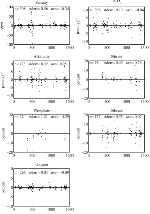
Figure 5. The difference between manually and automatically (with the running-cluster routine) performed crossovers for the CARINA-ATL data set. Numbers shown in the panels are the num-ber of data points (n), the standard error (stderr), and the average
difference (ave).
5.1 Manual vs. automatic crossovers
Both manually and automatically generated crossovers were used for the analysis. In order to evaluate any biases
be-tween the two methods we have plotted the difference
be-tween manually performed crossovers vs. crossovers gener-ated automatically with the running-cluster routine for the Atlantic subset of CARINA in Fig. 5. The manual results are found in the crossover table on the CARINA website, see
be-low. These crossovers were generated by a number of diff
er-ent analysts, poter-entially using different maximal horizontal
length scales, clustering, minimum depth etc. Even though there are a number of data points that are significantly
dif-ferent from zero, the mean difference is close to zero for all
of parameters except phosphate. The few data points with
large deviations from zero difference are due to miss-entered
values in the crossover table and crossovers that were per-formed on few data points, i.e., that have low significance.
It is clear that there are some differences in the results from
the manually and automatically generated crossovers but that
the overall difference is small, although it could potentially
be important for some cruises.
5.2 Automatic crossover routines
The offsets determined by the two different automatic
crossover routines discussed above (Sects. 4.1.2 and 4.1.3) are compared to each other to evaluate any biases, Fig. 6. The first observation is that the cnaX routine generally found more crossovers than the RunningCluster (RC) routine. This is mostly due to the spatial distance within which to search for crossovers being larger for cnaX than for RC; cnaX will thus find more crossovers at an increased risk of introducing errors due to spatial variability. The second observation is that performance is different for different parameters. For
in-stance, determinations of oxygen-offsets by the two routines
are in agreement to approximately 1%, while silicate offsets
are determined with a much lower agreement of about 7 %
(measured as the standard deviation of the difference from
the two methods), Fig. 6. Given that each routine operates
equally for all parameters, the cause for the difference must
be the silicate data itself. Profile interpolation is assumed not to be cause of the problem since the vertical sample distribu-tion is in most cases identical for nutrients and oxygen, both generally being sampled at full resolution. A possible cause of the difference is high station-to-station variability of
sili-cate values either due to analytical difficulties or large
natu-ral variability of silicate values in the deep water. This would
make the result of the offset determinations strongly
depen-dent on the stations included in the crossover. The second
alternative is certainly possible considering the large diff
er-ence in silicate concentrations in the southern and northern end-members of the Atlantic deep waters. In this case the
different “search radius” would be important for the result.
On the other hand, offsets determined for alkalinity are in
very good agreement between the two routines, suggesting that although large biases between cruises exist for this pa-rameter, the alkalinity values within a cruise is measured with a constant bias.
Taking the RMSE of the difference between the offsets
de-termined by the two routines as an upper limit of detection for biases, we conclude that the thresholds used by the CA-RINA team for applying adjustments are on the optimistic side for silicate and phosphate, about right for oxygen,
ni-trate, salinity and TCO2, and too conservative for alkalinity,
Table 2.
5.3 Adjustments
−50 0 50 −50
0 50
cnaX offsets
NRC=661 NcnaX=825 N
RC&cnaX=626
R2: 0.67 rmse: 7.65 Salinity [ppm]
−20 −10 0 10 20 −20
−10 0 10 20
NRC=350 NcnaX=352 N
RC&cnaX=213
R2: 0.57 rmse: 3.61 TCO
2 [umol/kg]
−20 0 20
−30 −20 −10 0 10 20 30
NRC=234 NcnaX=317 N
RC&cnaX=211
R2: 0.93 rmse: 2.88 TA [umol/kg]
−20 −10 0 10 20 −20
−10 0 10 20
RC offsets NRC=429 NcnaX=584 N
RC&cnaX=410
R2: 0.78 rmse: 2.90 NO
3 [%]
−20 −10 0 10 20 −20
−10 0 10 20
RC offsets
cnaX offsets
NRC=430 NcnaX=529 NRC&cnaX=397
R2: 0.85 rmse: 4.23 PO
4 [%]
−20 −10 0 10 20 −20
−10 0 10 20
RC offsets NRC=457 NcnaX=583 NRC&cnaX=416
R2: 0.44 rmse: 6.95 Si [%]
−10 −5 0 5 10
−10 −5 0 5 10
RC offsets NRC=509 NcnaX=641 NRC&cnaX=484
R2: 0.87 rmse: 1.09 O
2 [%]
Figure 6.Figure comparing offsets determined by the cnaX method and the Running-Cluster (RC) method for the SO and ATL areas (black dots with gray error bars). The square in the middle of the figures indicate the minimum adjustment that were applied to the data. The
numbers in the upper left corner states the number of crossover that the different methods found; the numbers in the lower right corner states
the R2value of the linear fit and and the rmse of the difference between the methods. The methods are generally in good agreement, with the
exception for silicate, where the standard deviation of differences between the two methods is around 7%. See text for discussion.
Table 3. The internal consistency of the data set expressed as the
weighted mean of the absolute offsets for all crossovers in
CA-RINA. Various levels of consistency are acquired by applying vary-ing corrections to the dataset: Uncorrected, before any adjustments
are applied; Limited, no adjustments smaller than the cut-offlimit
(see Table 2) are applied; Unlimited, all corrections suggested by the inversion are applied. The statistics are determined by the cnaX routines using all crossovers from the complete CARINA data set.
Parameter Uncorrected Limited Unlimited
Oxygen [%] 1.6 0.8 0.6
Nitrate [%] 3.5 1.7 1.4
Silicate [%] 6.2 2.8 2.6
Phospate [%] 5.1 2.5 2.4
TCO2[µmol/kg] 5.0 3.2 2.6
TAlk [µmol/kg] 6.7 3.9 2.5
Salinity [ppm] 6.1 4.0 3.3
the effects of the threshold, we analyzed how the weighted
mean offsets for all crossovers and parameters in the
CA-RINA data set are affected by using two different sets of
ad-justments; in the first case all the corrections suggested by the inversion were blindly applied to all the data, in the second case we applied only adjustments larger than the threshold (see Table 2). The overall performance is somewhat better
if all corrections are applied, Table 3, but the difference
be-tween the two cases is not particularly large. Thus, appli-cation of all corrections suggested by the inversion results in the most internally consistent dataset, but implicitly sug-gests a confidence in the adjustments that is not warranted for a relatively small gain in internal consistency. An exam-ple of the effect of the adjustments on the offsets for
individ-ual crossovers can be seen in Fig. 7 where the offsets of all
crossovers for alkalinity are plotted; before any adjustments are applied as well as after adjustments larger than the
thresh-old are applied. The mean absolute offset clearly decreases
by application of the adjustments.
We have also directly compared the suggested corrections derived from the cnaX scripts with the adjustments that were actually applied to the CARINA data product, Fig. 8. The
differences between the corrections and adjustments are a
0 100 200 300 400 500 600 700 800 −40
−30 −20 −10 0 10 20 30 40
Additive offsets for TA for all crossovers of all cruises
Mean offset (s.d.) before adjustments: −0.0085638 (10.094) Mean abs. offset before adjustments: 7.3786
Mean offset (s.d.) after adjustments: −1.3722 (6.3691) Mean abs. offset after adjustments: 4.7865
o − offset before adjustments (with uncertainty) x − offset after adjustments
Crossover number
Offset at crossover [umol/kg]
Histogram
Relative frequency
Figure 7. Figure showing the offsets for individual crossovers for alkalinity as determined by the cnaX routine. The gray circles are the
offsets before adjustment; black crosses the offsets after application of the adjustments suggested by the inversion that are larger than the
threshold value. Both sets of offsets are sorted independently of each other, but the uncertainty of the crossovers is only shown for the
uncorrected crossovers. The right panel shows the relative distribution of offsets (gray line before adjustment; black line after adjustment).
This analysis includes also the GLODAP reference cruises.
−50 0 50
−50 0 50
cnaX−suggested corrections
Salinity [ppm]
N carina=12 NcnaX=143 Nboth=10
R2: 0.88 rmse: 6.93
−20 −10 0 10 20 −20
−10 0 10 20
TCO2 [umol/kg]
N carina=27 NcnaX=91 Nboth=15
R2: 0.79 rmse: 6.23
−20 0 20
−30 −20 −10 0 10 20 30
TA [umol/kg]
N carina=25 NcnaX=77 Nboth=23
R2: 0.91 rmse: 3.56
−20 −10 0 10 20 −20
−10 0 10 20
CARINA adjustment NO3 [%]
N carina=29 NcnaX=117 Nboth=25
R2: 0.89 rmse: 2.19
−20 −10 0 10 20 −20
−10 0 10 20
CARINA adjustment
cnaX−suggested corrections
PO4 [%]
Ncarina=33 NcnaX=116 Nboth=30
R2: 0.89 rmse: 2.80
−20 −10 0 10 20 −20
−10 0 10 20
CARINA adjustment Si [%]
Ncarina=31 NcnaX=116 Nboth=24
R2: 0.83 rmse: 5.75
−10 −5 0 5 10
−10 −5 0 5 10
CARINA adjustment O2 [%]
Ncarina=42 NcnaX=125 Nboth=38
R2: 0.83 rmse: 1.49
Figure 8.A comparison between the corrections suggested by the cnaX routine and the adjustments applied to the CARINA data product. Black dots denote that an adjustment was applied; black crosses that no adjustment was applied. The square in the middle of the figures indicate the minimum adjustment that were applied to the data. The numbers in the upper left corner states the number of cruises for which
a correction was suggested by the cnaX method (NcnaX) and the number of adjustments applied to the CARINA data (Ncarina); the numbers in
the lower right corner states the R2value of the linear fit and and the rmse of the difference between the methods for those cruises where an
true, although not as often, i.e. even if the inversion suggests a correction smaller than the threshold, an adjustment has been made. Further inversions could have been performed (with the adjusted system) to find new model solutions that iteratively maximizes the internal consistency of the system. A first step in this iterative process was taken, but as we found that the result did not significantly improve the result above the level of uncertainty, this was not further pursued.
6 The web-based crossover workspace
The CARINA team included a large number of scientists from all over the world working simultaneously on the
qual-ity control and rapid communication of individual efforts and
results were important for the success of the project. To fa-cilitate this, an interactive internet based platform was de-veloped. To the user, the website provides important func-tions and tables of which the crossover and adjustment ta-bles are the most important. We will first briefly discuss some of the functionality of the website from a user’s per-spective, and will then describe its basic architecture. A non-user interactive version of the website, with all the in-formation used by the CARINA team, is available at http:
//cdiac.ornl.gov/oceans/CARINA/Carina inv.html.
The crossover table provides the interface to enter off
-set values for crossovers for any of the 14 parameters con-sidered for the secondary QC. Also generic information to a crossover, such as position, number of stations etc. can be entered. Furthermore, files can be uploaded and com-ments can be posted. This allows several investigators to work on crossover analysis simultaneously without duplicat-ing work and enables communication of information. The adjustment table is similar in its functionality. Adjustment values, files and comments can be entered or uploaded for any of the 14 parameters, or to the cruise as a whole. Further-more, a quality flag (either “good” or “poor”) is assigned for
each cruise/parameter combination. The user can search the
database for all figures relevant to a cruise/parameter
com-bination, and create a link to the adjustment table. This al-lows the investigator to select important figures that motivate the choice of adjustment. There is also a link to the relevant readme (i.e. condensed cruise metadata) for each cruise entry in the adjustment table.
The cruise and ship tables provide easy access to basic information for each cruise or ship, if that information is not found in the readme files. More importantly, it provides means to keep track of the aliases for different cruises, i.e. old versions of the EXPOCODE or project names associated to a cruise (this information is also displayed in the adjustment table). The information in the crossover and adjustment ta-bles can be exported as csv-files that can be used by other applications. For instance, the adjustments are used for cre-ation of the merged data product where the adjustments in the table are applied to the data in the individual cruise files,
or the manually entered crossover values can be downloaded for the inversions. Another important aspect of the website is the possibility to post larger files and data volumes. This en-able, for instance, rapid upload of inversion results that can-not be attributed to any specific cruise. Also draft versions of manuscripts etc. were posted on the website.
The CARINA website project started with the initial quirement of at least two tables; one where crossover re-sults could be stored, and one for adjustment values of in-dividual cruises. Supplemental information such as figures, comments and ReadMe files could be stored on the plat-form as well and be linked to submitted data. It soon be-came clear that this website would accumulate thousands of individual data points for crossovers and adjustments, and even more supplementary files and updates of these. All of this would then have to be available to all users during the data compilation and evaluation process. Manual creation or maintenance of contents and links would thus be impossi-ble. Moreover, the need arose to batch submit a large num-ber of automatically generated figures and data calculated by user scripts which should be automatically processed and reflected throughout the applications. The greatest demand (and challenge) was the linkage between an individual da-tum and multiple supplementary information with the ability to “share” these relations in other contexts. For example, a supplemental file uploaded to the crossover analysis of salin-ity (which involves two cruises) should be available in the context of the salinity adjustment value for each of the two cruises, and whenever the file is updated it would have to be reflected in every shared relation. To accommodate these de-mands, we decided in favor of open source software in order to be able to freely use and distribute the application, partic-ularly after termination of this project and in case that offline usage is needed. We chose to use Ruby on Rails, which is based on the object-oriented programming language Ruby, as web application framework and PostgreSQL as relational database for storage of data and information snippets. Up-loaded files are stored in the file-system, while their respec-tive metadata are kept in the database.
According to the Ruby on Rails framework, the CARINA application is implemented using the model-view-controller architecture (MVC) which provides an out-of-the-box basic skeleton of all necessary methods to create, read, update or delete (CRUD) datasets of a particular model (i.e. a corre-sponding table) and to build HTML forms or pages to edit or display datasets in the end user’s browser. Due to the con-ventions of the Rails framework, all methods necessary for
a quick and effortless implementation of links between a
All information of the CARINA web application is stored in a total of eleven database tables: ships, countries, cruises, crossovers, regions, adjustments, attachments, comments, postings, readmes and users. Datasets are then handled by
Rails as objects with automatically created methods. This
provides access to both a dataset’s parameters (i.e. columns) and to other related datasets; these are also treated as ob-jects. This allows syntactically simple access to the
param-eters/attributes (i.e. columns) of datasets and their
supple-ments as well as to the relations between different models.
It also avoids formulation of any SQL-based queries or han-dling of interactions with the back-end database. We have used polymorphic relations for comments, readmes, postings and attachments. This allows a single model (e.g. attachment representing an uploaded file) to be used for datasets of dif-ferent models to which files can be uploaded (i.e. attached). In the CARINA site, most models can thus have multiple files uploaded to a single dataset. We even extended this fea-ture by an additional attribute for attachment and comment records holding the parameter to which an uploaded file or a comment is attached. Thus, a file uploaded to a crossover can be specifically “attached” to any parameter, for instance salinity.
In numerous cases crossovers are assigned to more than one working group (see Sect. 2 on data provenance). It was required that each working group could store values for their regional crossover separately. This is accomplished by in-sertion of two additional crossovers as subsets with a simple parent-child relation to the parental crossover (parent id as foreign key) representing the two data provenances. Mem-bers of either working group can click a dynamically inserted link in the list view whenever subsets are present and both subsets are then retrieved from the server and displayed in the context without reloading the entire page. One of the subsets is always assigned as primary subset yielding a pri-ority for automatic display of values; as long as a parameter value is not finalized and entered in the primary (i.e. parent) dataset, the web application displays the value of the param-eter from the primary subset or, if no value has been entered, from the secondary subset. A trailing “c” as subscript to the value indicates such a copy. Another parent-child relation is used for the adjustments table when a cruise or campaign may have to be split in sections due to temporal variations in the proper adjustment value (e.g. mid-cruise change of
stan-dards or different instrument performance after a port call).
In this case multiple copies of the dataset are inserted, but as there is no unique solution to this case, multiple datasets are either exported or displayed and sorted according to the sets of stations which apply.
All authenticated users can upload files individually via the web-interface and some authorized users can upload di-rectly into a separate folder accessible via WebDAV. This al-lows uploads of large file batches created by script routines
which, when compliant with naming and file/folder hierarchy
conventions, can be ingested upon request of the uploading
user, and will “attach” each discovered plot file to the appro-priate crossover (or adjustment). Uploaded figures are com-monly provided in PostScript format, unsuitable for display in web browsers. These files are automatically converted to PNG formatted files using the ImageMagick utilities and available for quick views of the figure via an autogenerated weblink while the original PostScript file is only sent to the user when a download is explicitly requested. Special forms allow users to make a selection of crossovers or adjustments which they wish to export and download. An entry which is not a number may be exported as a string (e.g. NaN) or as a
special number (e.g.−999) based on individual user settings.
Similarly, overview lists of all comments posted to each ad-justment can be generated and saved to disk.
Overall statistics reflect busy usage of the CARINA work-ing platform: 2102 crossovers (with additional 556 sub-sets to 278 crossovers), 238 cruises and respective adjust-ment datasets, 35 063 attached plot files, 1919 comadjust-ments, 173 readmes and 107 postings, all together consuming about 10 Gigabytes of disk space.
Acknowledgements. This work has been performed and funded as part of the EU project CarboOcean (Project
511176-2). Additional support from the International Ocean Carbon
Coordination Project IOCCP (Maria Hood) and the Hanse Institute for Advanced Study (HWK Delmenhorst, Germany)
are gratefully acknowledged. Additional support provided as
follows for: R. M. Key, NOAA grant NA08OAR4320752 and NA08OAR4310820; A. Velo, PGIDIT05OXIC40203PM Xunta de
Galicia and CTM200627116E/MAR MEC; A. Olsen NFR grant
178167, A-CARB.
Edited by: V. Gouretski
References
Gouretski, V. V. and Jancke, K.: Systematic errors as the cause for an apparent deep water property variability: global analysis of the WOCE and historical hydrographic data, Prog. Oceanogr., 48, 337–402, 2001.
Johnson, G. C., Robbins, P. E., and Hufford, G. E.: Systematic
adjustments of hydrographic sections for internal consistency, J. Atmos. Ocean. Technol., 18, 1234–1244, 2001.
Key, R. M., Kozyr, A., Sabine, C. L., Lee, K., Wanninkhof, R., Bullister, J. L., Feely, R. A., Millero, F. J., Mordy, C., and Peng, T. H.: A global ocean carbon climatology: Results from Global Data Analysis Project (GLODAP), Global Biogeochem. Cy., 18,
GB4031, doi:1029/2004GB002247, 2004.
Key, R. M., Tanhua, T., Olsen, A., Hoppema, M., Jutterstr¨om, S., Schirnick, C., van Heuven, S., Kozyr, A., Lin, X., Velo, A., Wal-lace, D. W. R., and Mintrop, L.: The CARINA data synthesis project: introduction and overview, Earth Syst. Sci. Data Dis-cuss., 2, 579–624, 2009,
Lamb, M. F., Sabine, C. L., Feely, R. A., Wanninkhof, R., Key, R. M., Johnson, G. C., Millero, F. J., Lee, K., Peng, T. H., Kozyr, A., Bullister, J. L., Greeley, D., Byrne, R. H., Chipman, D. W., Dickson, A. G., Goyet, C., Guenther, P. R., Ishii, M., Johnson, K. M., Keeling, C. D., Ono, T., Shitashima, K., Tilbrook, B., Takahashi, T., Wallace, D. W. R., Watanabe, Y. W., Winn, C., and Wong, C. S.: Consistency and synthesis of Pacific Ocean CO2 survey data, Deep-Sea Res. Pt. Ii-Top St Oce, 49, 21–58, 2002.
Ronski, S. and Bud´eus, G.: Time series of winter
convec-tion in the Greenland Sea, J. Geophys. Res., 110, C04015,
doi:10.1029/2004JC002318, 2005.
Sabine, C. L., Key, R. M., Johnson, K. M., Millero, F. J., Poisson, A., Sarmiento, J. L., Wallace, D. W. R., and Winn, C. D.:
Anthro-pogenic CO2inventory of the Indian Ocean, Global Biogeochem.
Cy., 13(1), 179–198, 1999.
Sabine, C. L., Key, R. M., Kozyr, A., Feely, R. A., Wanninkhof, R., Millero, F., Peng, T. H., Bullister, J., and Lee, K.: Global Ocean Data Analysis Project (GLODAP): Results and Data, NDP-083, Carbon Dioxide Information Analysis Center, Oak Ridge Na-tional Laboratory, US Department of Energy, Oak Ridge, TN, 2005.
Tanhua, T., Steinfeldt, R., Key, R. M., Brown, P., Gruber, N., Wan-ninkhof, R., Perez, F., K¨ortzinger, A., Velo, A., Schuster, U., van Heuven, S., Bullister, J. L., Stendardo, I., Hoppema, M., Olsen, A., Kozyr, A., Pierrot, D., Schirnick, C., and Wallace, D. W. R.: Atlantic Ocean CARINA data: overview and salinity adjust-ments, Earth Syst. Sci. Data Discuss., 2, 241–280, 2009,
http://www.earth-syst-sci-data-discuss.net/2/241/2009/.