www.geosci-model-dev.net/5/1425/2012/ doi:10.5194/gmd-5-1425-2012
© Author(s) 2012. CC Attribution 3.0 License.
Geoscientific
Model Development
Mass-flux subgrid-scale parameterization in analogy with
multi-component flows: a formulation towards scale independence
J.-I. Yano
GAME/CNRM, CNRS-INSU-M´et´eo France, URA1357, Toulouse, France
Correspondence to: J.-I. Yano ([email protected])
Received: 6 October 2011 – Published in Geosci. Model Dev. Discuss.: 24 November 2011 Revised: 13 May 2012 – Accepted: 26 October 2012 – Published: 21 November 2012
Abstract. A generalized mass-flux formulation is presented, which no longer takes a limit of vanishing fractional areas for subgrid-scale components. The presented formulation is applicable to a situation in which the scale separation is still satisfied, but fractional areas occupied by individual subgrid-scale components are no longer small. A self-consistent for-mulation is presented by generalizing the mass-flux formu-lation under the segmentally-constant approximation (SCA) to the grid–scale variabilities. The present formulation is ex-pected to alleviate problems arising from increasing resolu-tions of operational forecast models without invoking more extensive overhaul of parameterizations.
The present formulation leads to an analogy of the large-scale atmospheric flow with multi-component flows. This analogy allows a generality of including any subgrid-scale variability into the mass-flux parameterization under SCA. Those include stratiform clouds as well as cold pools in the boundary layer.
An important finding under the present formulation is that the subgrid-scale quantities are advected by the large-scale velocities characteristic of given subgrid-scale components (large-scale subcomponent flows), rather than by the total large-scale flows as simply defined by grid-box average. In this manner, each subgrid-scale component behaves as if like a component of multi-component flows. This formulation, as a result, ensures the lateral interaction of subgrid-scale variability crossing the grid boxes, which are missing in the current parameterizations based on vertical one-dimensional models, and leading to a reduction of the grid-size depen-dencies in its performance. It is shown that the large-scale subcomponent flows are driven by large-scale subcompo-nent pressure gradients. The formulation, as a result,
further-more includes a self-contained description of subgrid-scale momentum transport.
The main purpose of the present paper is to appeal the importance of this new possibility suggested herein to the numerical weather forecast community with im-plications for the other parameterizations (cloud fraction, mesoscale organization) as well as resolution-dependence of parameterizations.
1 Introduction
The present paper presents a generalization of the mass-flux parameterization formulation for representing non-convective processes as well as convection. As a side prod-uct, we also provide an answer to the following question: Are the subgrid-scale parameterized variables advected by large-scale flows? This is one of the typical questions often asked in a context of operational implementation of a subgrid-scale process parameterization. The present paper shows that it is the corresponding subcomponent large-scale flow that ad-vects a given subgrid-scale component variable, but not the whole large-scale flow. Importance of analogy of the mass-flux based parameterization with the multi-component flows is emphasized in order to better understand this conclusion.
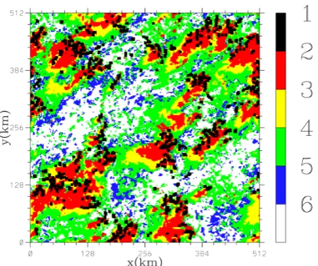
Fig. 1. Spatial distribution of six subgrid-scale categories over a domain of the sizes, 512 km×512 km, simulated by a cloud-resolving model (CRM). The categories are (1) precipitating con-vection, (2) precipitating stratiform, (3) non-precipitating strati-form, (4) shallow clouds, (5) ice anvils, and (6) environment. The CRM simulation is from the TOGA-COARE (Tropical Ocean Global Atmosphere Couple Ocean Response Experiment) period, representing a typical fully-developed marine-type deep convective system. See Yano et al. (2005) for details of the simulations as well as the categorization scheme. (From Fig. 2a of Yano et al. (2005) with modifications).
subscale elements remain much smaller than the grid-box size, a fractional area occupied by each category of subgrid-scale processes is no longer substantially smaller than the grid-box size.
An example of such a situation is shown in Fig. 1 taken from Fig. 2a of Yano et al. (2005) with modifications. Here, we show a spatial distribution of five cloud categories over a typical size of a grid box for global climate modelling, 512 km×512 km, simulated by a cloud-resolving model (CRM). The categories show (1) precipitating convection, (2) precipitating stratiform, (3) non-precipitating stratiform, (4) shallow clouds, and (5) ice anvils. The remainder, cate-gory (6), is considered the “environment”. The CRM simu-lation is from a TOGA-COARE (Tropical Ocean Global At-mosphere Couple Ocean Response Experiment) period, rep-resenting a typical fully developed marine-type deep convec-tive system. We refer to Yano et al. (2005) for details of the simulations as well as the categorization scheme.
Individual precipitating convective elements (category 1) occupy only very small fractional areas in the grid box, being consistent with the scale separation principle as assumed in the standard mass-flux parameterization. The stratiform-type clouds, on the other hand, tend to take larger fractional areas individually, and looking them as a whole category, the occu-pied area is no longer substantially smaller than the grid-box size. Even for precipitating convection, the total fractional
area is not as small as that for the individual convective ele-ments, because they are numerous. Most importantly, the en-vironment does not occupy the majority of the grid box at all, but its fractional area is just comparable with any stratiform-type cloud regions.
The present paper is going to present a formulation for this type of situation in subgrid-scale parameterization un-der a mass-flux based approach. The situation to be consid-ered is a drastic departure from the approximations adopted by the standard mass-flux subgrid-scale parameterization, as established by Arakawa and Schubert (1974): (1) frac-tional areas occupied by individual subgrid-scale compo-nents (convective-plume types) are much smaller than unity; (2) the environment (non-convective area) occupies a major-ity of the grid-box domain; and (3) all the subgrid-scale com-ponents are exclusively surrounded by the environment.
In contrast, the situation considered in the present work is (1) fractional areas occupied by individual subgrid-scale components are no longer much smaller than unity; (2) the environment (non-convective area) no longer occupies a ma-jority of the grid-box domain; and as a result, (3) subgrid-scale components are no longer exclusively surrounded by the environment, but more than often adjacent with the other subgrid-scale components.
Importance of such generalization in the mass-flux based parameterization cannot be overemphasized. First of all, un-der this situation, the traditional mass-flux formulation leads to erroneous results.
In order to see this point, let us take the environmental vertical velocity (typically an environmental descent), we,
as an example. The basic idea of mass-flux convection pa-rameterization is to divide the grid-box domain into con-vection and the environment. For simplicity, let us assume only one type of convection is found within a given grid box. Let a fractional area occupied by convection within the grid boxσc, then the environment occupies a fractional area,
1−σc. As a result, for example, the vertical velocity,w, is
divided into the two parts, those coming from convection,
wc, and those coming from the environment,we. The total
vertical velocity is obtained by taking a weighted sum of the two:w=σ wc+(1−σc)we. Conversely, the environmental
vertical velocity is given by
we=
w−σcwc
1−σc
. (1)
Under the standard approximation, we take σc1, thus
Eq. (1) reduces to
we'w−σcwc. (2)
However, when the fractional area satisfiesσc∼1, Eq. (2)
obviously underestimates the environmental subsidence compared to the exact Eq. (1).
is no longer satisfied. All the formulations must be rewrit-ten thoroughly. The most important consequence is that the grid-box mean for the thermodynamic variables can no longer be equated with the environmental values as assumed in the standard formulation. Also for this very reason, the substantial reformulation of the problem is required.
However, in order to enable such a reformulation, we also require an appropriate general framework. For this purpose, we take a unified approach for the subgrid-scale physical pa-rameterization in terms of the mode decomposition proposed by Yano et al. (2005). The basic idea of this approach is to take a full physical system, such as a cloud-resolving model (CRM) or a large eddy simulation (LES) for subgrid-scale variables as a starting point, and apply a mode decomposi-tion to these subgrid-scale variables in order to further sim-plify the physical description (i.e. model “compressions”).
Under this unified approach, the mass-flux parame-terization can be reinterpreted as a formulation under the segmentally-constant mode decomposition. Under this framework, the subgrid-scale variables are approximated by a segmentally-constant approximation (SCA), as pointed out by Yano et al. (2010a). Here, each subgrid-scale physical component is assumed to be consisting of horizontally homo-geneous distribution of physical variables within each sub-component.
That is essentially a geometrical constraint imposed on an ensemble of convective updrafts in developing the standard mass-flux formulation (cf. Arakawa and Schubert, 1974). Under the present generalization, not only the convective up-drafts, but any subgrid-scale components can be represented under this geometrical constraint, SCA. The mode decompo-sition provides a basis for subgrid-scale physical representa-tions, because the method can “compress” the physical sys-tem a great deal when an appropriate set of decomposition modes is chosen. SCA loosely corresponds to when the Haar wavelet is chosen as a set of decomposition modes. The effi-ciency of this choice, along with the other choices of wavelet, is well demonstrated in Yano et al. (2004b). See their Figs. 5 and 8 as graphical demonstrations for the efficiency of SCA. In this respect, it is important to emphasize that the present paper does not at all intend an improvement of any ex-isting schemes, but it proposes a completely new parame-terization formulation. A general applicability of the pro-posed formulation cannot be overemphasized being based on a very general framework without specifying any partic-ular situations, although without doubt, the present author’s motivation stems from the tropical atmospheric dynamics as summarized by Fig. 1.
The present formulation is so general that it does not even specify which physical processes must be represented un-der the mass-flux framework. The choice is totally left to the readers who are going to develop their own schemes un-der the proposed general formulation. For this very reason, though the proposed formulation is closed mathematically, it is left open physically in order to maintain its generality.
Benefits of this kind of generalization is hardly overem-phasized. It first of all enables us to to consider mesoscale convective organization (cf. Moncrieff, 1995) under the mass-flux framework. The mesoscale convective organiza-tion is clearly a structure comparable in size with the grid box even for a relatively low-resolution climate model. The proposed formulation provides a way of incorporating these processes as an integrated part of the mass-flux formulation. The best effort so far towards this goal, in the best knowl-edge of the author, is by Donner (1993), who indeed includes the mesoscale effects as a part of his mass-flux convection parameterization. However, the mesoscale effect itself is not formulated by mass flux, but simply added as an appendix.
Applications of the proposed formulation are even not lim-ited to the convective processes. The formulation can also be applied to various non-convective processes such as strati-form clouds, cold pools in the boundary layer. Thus, it in-cludes the cloud-fraction parameterization within its scope, for example. In short, any subgrid-scale physical processes can be incorporated into the proposed framework so long as the process in concern is associated with a geometrical entity well represented under SCA.
However, as an important consequence of this modifica-tion, the “environment” no longer represents a special status but just reduces to one of many possible subgrid-scale com-ponents. Under the present formulation, every subgrid-scale component is described by a prognostic equation system akin to the fully physical system taken as a starting point. The grid-box averaged quantity is no longer equivalent to the en-vironmental state, as the traditional parameterizations would assume, but it is only available by taking a weighted average of all the subgrid-scale component variables.
In order to perform a required modification and a gener-alization to the mass-flux parameterization, a point of view taken is one advocated by Yano et al. (2005, 2010a) that the mass-flux convection parameterization can be considered as a consequence of an application of segmentally-constant approximation (SCA) to a full physical system. The idea of SCA consists in subdividing a grid box domain into a num-ber of constant value segments in different sizes and shapes as suggested by Fig. 1. SCA can be considered as a geo-metrical constraint applied to a full physical system in order to construct the mass-flux based parameterization in a more general manner. Recall that the standard mass-flux formu-lation is constructed by assuming SCA for convective up-drafts and the remaining environment. Any subgrid-scale components likely to be approximated by horizontal homo-geneity inside each component (e.g. stratiform clouds, cold pools in the boundary layer) can also be included into this SCA formulation.
developing a formulation, we take the hydrostatic primitive equation system. Some justifications for this choice are given in the beginning of Sect. 2.2. A full development of SCA un-der a non-hydrostatic formulation is left for a future study due to its associated extensive complexities.
The mass-flux parameterization developed under the present formulation presents a special flavor with a close link to a traditional description of multi-component flows. This aspect is discussed in the first half of the next section. The remainder of the next section is devoted to introducing the primitive equation system that is taken as a starting point for applying SCA. Section 3 is devoted to a stepwise reduction of the full system under the application of SCA. The ob-tained set of equations is discussed in Sect. 4. Discussions include not only various formulational details and possible applications, but further implications from the present work including construction of a scale-independent parameteriza-tion. The paper is concluded in Sect. 5. Some mathematical details are deferred to the Appendix.
2 Preliminaries
2.1 Analogy with multi-component flows
The basic idea of mass-flux parameterization may be under-stood as that of a multi-component system with each sub-component designated by subscript j. A colloidal system such as milk is such an example. Milk consists of many “bub-bles” of water and fats, which are not visible on a macro-scopic scale (i.e. large scale or grid scale), but which should appear on the microscale (i.e. subgrid scale). Thus, in order to describe the macroscopic evolution of milk (flow), we have to specify the fractional volume occupied by water and fats, re-spectively, at every macroscopic point. The fractional volume is the counter concept for the fractional area,σj, occupied by thej-th subcomponent in the mass-flux formulation. From this perspective, a review on multi-component fluid systems given, for example, by Gyarmati (1970) is fruitful for better understanding the principle of mass-flux parameterization.
The situation can be understood under a mathematical symbolism as follows. Let the characteristic scales for the macroscopic (resolved) and microscopic (unresolved) pro-cesses be 1X and 1x, respectively. Separation between macroscopic and microscopic processes suggests
1X1x.
The key starting point for constructing a subgrid-scale physical parameterization is to make a clear decision which belongs to the resolved scale,1X, and which belongs to the subgrid scale,1x. This distinction may be best made by tak-ing an analogy with macroscopic and microscopic processes, though the scale separation between these two scales may not be as well separated as a typical multi-component flow. The current subgrid-scale parameterizations often suffer from the
problems of resolution dependence. A part of the problem may be attributed to the fact that there is no clear definition of what the scale of the large scale flow represented by the model, thus what must be parameterized.
Moreover, the meteorological subgrid-scale parameteri-zation problem is more complex than a standard multi-component flow, because there is an exchange of mass be-tween the different subcomponents. For example detrained air from a cumulus cloud can turn into a part of a strat-iform cloud. This is a situation normally not expected in fluid-mechanical multi-component flows: in milk, water al-ways remains water and fats alal-ways remain fats. Chemi-cal reactions are the only expected means that one subcom-ponent turns into another in these multi-comsubcom-ponent flows (cf. Gyarmati, 1970).
In order to fully take into account these complex pro-cesses in the subgrid-scales, the most straightforward math-ematical approach would be to adopt that of the multi-scale analysis as pointed out by Majda (2007a, b) and as applied by Xing (2009). Under this approach, the coordi-nates for the two scales are introduced, those, say,(x, y) de-scribing the subgrid-scales and those(X, Y ) describing the large-scale (grid-scale). General coordinates may be given by(x+X/, y+Y /)withbeing a small parameter, which may be taken as 1x/1X. By taking an asymptotic limit,
→0, the subgrid-scale variability described by the coordi-nates(x, y)shrinks into a single “macroscopic” point in re-spect to the large-scale (grid-scale) coordinates(X, Y ). That is the basic notion behind the scale separation principle.
In the present paper, we take a slightly different approach, in which all the physical variables are consistently consid-ered under averaging over the grid box with a grid box size,
L. As a reminder for this averaging operation, we put a bar to the nabla,∇¯, when the nabla operator is considered in terms of the grid-box average.
From a numerical point of view, the grid-box size must be sufficiently smaller than typical macroscopic pro-cesses, because otherwise they are not numerically properly represented. Thus,
1XL. (3)
We have to realize that from the above argument that the grid-box size,L, is not at all constrained by the subgrid-scale,
1x. Here, only for the sake of considering the grid-box size as a reference scale for defining the “large scale”, or the grid scale against the subgrid scale, we will implicitly assume
L1x
in reminder of the paper. Here,Lin the above inequality may better be interpreted as a virtual grid size rather an actual one. As just stated, the actual grid size does not have to satisfy this constraint.
component variables are also functions of large-scale (grid-scale) coordinates. In other words, they should vary from one grid box to another. Implication from the scale separation principle (cf., Yano , 2009) is that these subgrid-scale com-ponent variables must, furthermore, vary smoothly from one grid box to another, because otherwise smoothness of a large-scale (grid-large-scale) solution is not guaranteed. This large-scale sep-aration issue turns out to be key in properly developing any parameterization.
2.2 A basic set of equations: hydrostatic primitive equation system
In order to develop a generalized mass-flux formulation in a heurestic manner from a basic set of equations, we adopt the hydrostatic primitive equation system as the latter. This choice may look hardly justifiable in light of the fact that the subgrid-scale processes in concern could be highly non-hydrostatic. However, here, we emphasize that parameteriza-tion is only concerned with feedback of these subgrid-scale variability to grid-box average. Most importantly, although individual subgrid-scale processes may be much faster than those of the grid scales, evolution of each subgrid-scale com-ponent defined in terms of an “ensemble” average over the grid box would have a characteristic time-scale compara-ble to those of the grid-scale processes. As a result, we can suppose that the non-hydrostatic effects, such as local accel-eration of vertical velocity, would become small by taking grid-box average. As will be emphasized below, the non-hydrostatic contributions of the subgrid-scale processes will be integrated into the entrainment-detrainment term under the present formulation.
For these reasons as well as for simplifying the formula-tion, we neglect the explicit nhydrostatic effects from on-set in the present study. Recall that Yanai et al. (1973) also developed their mass-flux formulation for observational di-agnoses from the primitive equation under pressure coordi-nate. The use of the primitive equation system is also con-sistent with the aim of applying the present formulation to the numerical weather forecast and climate change. At the same time, the ultimate importance of the non-hydrostatic processes in many atmospheric subgrid-scale processes can-not be overemphasized either. Unfortunately, those consid-erations turn out be rather involved, thus they are left for a future study.
Notice that this argument applies only when the total frac-tional area,σj, occupied by aj-th category is the order of unity. When the fractional area is small, a simple scale analy-sis suggests that the subcomponent vertical velocity must be scaled bywj∼σj−1, thus the local acceleration associated with vertical motion would no longer be negligible. An obvi-ous such process is deep convective towers (cf. Sect. 4.7).
The primitive equation system under the pressurep verti-cal coordinate consists of the horizontal momentum equation
∂
∂tu+ [∇ ·(uu)] + ∂
∂pωu= −∇φ+Fu, (4a)
the hydrostatic balance
∂
∂pφ= −α, (4b)
the mass continuity
∇ ·u+ ∂
∂pω=0, (4c)
and the heat equation
∂
∂tθ+ ∇ ·(uθ )+ ∂
∂pωθ+ω ∂θ0
∂p =Q. (4d)
Note that the second term of the left-hand side of Eq. (4a) is a short-handed expression with the exact form defined by Eq. (A2) withσj=1.
Here,uis a horizontal velocity,ωa vertical velocity (pres-sure velocity),φthe geopotential, and∇ designates the gra-dient operator over a constant pressure surface. In the hori-zontal momentum equation (Eq. 4a), all the other forces (e.g. Coriolis force) other than pressure gradient are simply desig-nated together asFu.
In the hydrostatic balance, the perturbation specific vol-ume α is related to the potential temperature perturbation
θby
α=(R/p)(p/p0)κθ,
where R is the gas constant, κ=R/Cp with Cp the specific heat with constant pressure, p0=1000 hPa
a reference pressure.
In the thermodynamic equation (Eq. 4d),Qis the total di-abatic heating rate,θ0is the reference state for the potential
temperature, which is assumed to be a function of pressure only. For economy of presentation, we omit the prime rep-resenting a deviation from a reference state. As a result, for example, the total potential temperature is given byθ0+θ.
We may further consider, for example, the mixing ratios,
qµ, for various water types (vapor, liquid cloud, precipitating water, etc.) with subscriptµdesignating water types:
∂
∂tqµ= −∇ ·vqµ− ∂ωqµ
∂p +Sµ, (5)
whereSµis a source for the given water type. In general, we can write a prognostic equation for any physical variable, say
ϕin the form
∂
∂tϕ= −∇ ·vϕ− ∂ωϕ
∂p +F (6)
3 A general formulation for the subgrid-scale processes under SCA
Segmentally-constant approximation (SCA) represents an ensemble of subgrid-scale components, marked by an in-dexj (=1,2,· · ·), within a grid box domain by approximat-ing a full system with a correspondapproximat-ing ensemble of constant value segments (cf. Yano et al., 2005, 2010a). Thej-th sub-component occupies an area of Sj with a boundary desig-nated by∂Sj. As a result, the original full system reduces to a discrete set of equations describing evolution of these constant-segment values at each vertical level. As a result, each subgrid-scale component is described in an analogous manner as the each subcomponent of a multi-component flow is prognostically described.
These subcomponents may, for example, represent differ-ent cloud types as shown in Fig. 1 above. Thus, in case of Fig. 1, the six subcomponents are considered. Note that, as illustrated by Fig. 1, a subcomponent does not usually con-stitute a single enclosed element, but many enclosed sub-elements. For the derivation of the generalized mass-flux for-mulation under SCA, we focus on a generic prognostic equa-tion (Eq. 6) and the mass continuity (Eq. 4c). Both the mo-mentum equation (Eq. 4a) and the water mixing-ratio equa-tion (Eq. 5) can be considered as special cases of Eq. (6). 3.1 Prognostic equations
The equation for any prognostic variableϕ for aj-th sub-component is obtained by integrating Eq. (6) over an area
Sj occupied by thej-th subcomponent. The result is given by Eq. (29) of Yano et al. (2005) when the boundary∂Sj for thej-th subcomponent with the other components does not move with time. A two-dimensional case with a mov-ing subcomponent-boundary is given by Eq. (10) of Yano et al. (2010a). By generalizing these results, under a three-dimensional configuration with the moving subcomponent-boundary, a system under SCA is defined by
∂ ∂tσjϕj+
∂σj(ωϕ)j
∂p + 1 S
I
∂Sj
ϕb,j(u∗b,j− ˙rb,j)·dr=σjFj, (7)
where the average over thej-th subcomponent (segmentally-constant values) is given by e.g.
ϕj= 1
σjS
Z
Sj
ϕdxdy, (8a)
(ωϕ)j= 1
σjS
Z
Sj
ωϕdxdy, (8b)
and a fractional areaσj occupied by thej-th subcomponent is defined by
σj= 1
S
Z
Sj
dxdy. (8c)
Here, note that the contour integral in Eq. (7) and hereafter is performed in the counter-clockwise direction, andS is a grid-box size.
Furthermore,r˙b,j designates the rate of the movement of the subcomponent boundary,u∗b,jis a normal velocity to the boundary defined by
u∗b,j=ub,j−ωb,j
∂rb,j
∂p (9)
withrb,j designating the position of the boundary. The sub-script b designates the values at the subcomponent boundary. By following the standard mass-flux approximation (cf. Yano et al., 2004a), we approximate the vertical flux by
(ωϕ)j'ωjϕj.
Note that fluctuations within a subgrid-scale component-segment can easily be included by re-writing it
(ωϕ)j=ωjϕj+(ωj00ϕ 00 j)j,
where the double prime indicates a deviation of a variable from SCA within the given subcomponent segment, i.e.
ϕj00=ϕ−ϕj.
We refer to Soares et al. (2004), and Siebesma et al. (2007) for the treatment of these fluctuation terms. Note that though these contributions are not further considered in the present paper, they are no doubt crucial in defining the vertical fluxes in the boundary layer, and those should be included as a part of a source term,Fj, for any subgrid-scale components in Eq. (6) in the following.
3.1.1 Horizontal divergence term
The divergence (contour integral) term in Eq. (7) can be sep-arated into the three parts:
I
∂Sj
ϕb,j(u∗b,j− ˙rb,j)·dr=
I
∂S+j
ϕb,j(u∗b,j− ˙rb,j)·dr
+
I
∂Sj−
ϕb,j(u∗b,j− ˙rb,j)·dr+
I
∂Sb,j
ϕb,j(u∗b,j− ˙rb,j)·dr. (10)
The first two parts (∂Sj+and∂S−j) are inside the grid box, where the last part (∂Sb,j) is a contribution from the grid-box boundary.
As a result, ∂Sj− is given by a sum of sub-segments ∂Sj,i−
adjacent with subcomponents designated by the subscripti:
∂Sj−= X i={i}j
∂S−j,i. (11)
Here,{i}j≡ {i1, i2,· · · }designates a set of the
subcompo-nents that are directly adjacent with thej-th subcomponent. For both parts, we take an upstream approximation, as adopted by Asai and Kasahara (1967: their Eq. 3.29) as well as by Arakawa and Schubert (1974), thus
ϕb,j=
(
ϕj, (u∗b,j− ˙rb,j)ϕ·drj>0,
ϕi, (u∗b,j− ˙rb,j)ϕ·drj<0.
(12)
Note that the choice of the upstream approximation is purely a numerical issue. An equivalent formulation could be developed with any advection scheme. Nevertheless, we take the upstream approximation for the two princi-pal reasons. First, because it leads to a formulation with the closest analogy with the conventional mass-flux for-mulation (cf. Arakawa and Schubert, 1974). Second, the approach ensures the numerical stability of the horizontal advection calculations.
As a result, we introduce the detrainment and the entrain-ment rates by
dj= 1
S
I
∂Sj+
(u∗b,j− ˙rb,j)·dr, (13a)
ej,i= − 1
S
I
∂Sj,i−
(u∗b,j− ˙rb,j)·dr. (13b)
Substitution of Eqs. (12) and (13a,b) into Eq. (10) shows that the inflow and outflow fluxes provide
1
S
I
∂S+j
ϕb,j(u∗b,j− ˙rb,j)·dr=djϕj, (14a)
1
S
I
∂S−j,i
ϕb,j(u∗b,j− ˙rb,j)·dr= −ej,iϕi, (14b)
respectively.
Note that the detrainment and the entrainment rates,djand
ej,i, are only short-handed expressions for the more complete expressions in the right-hand side of Eq. (13a,b). These pa-rameters are also considered to express a contribution of non-hydrostatic processes not explicitly considered in the present formulation. At the same time, they remain the main param-eters left undetermined under the present formulation (cf. Sect. 4.4).
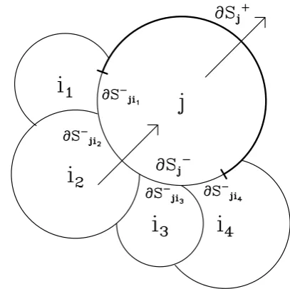
Fig. 2. Schematics for showing the definitions of the boundary seg-ments for thej-th subgrid component. Here, the boundary is first divided into the two parts: those associated with the outflow,∂S+j, and those associated with the inflow,∂Sj−. In the figure, the out-flow segment,∂Sj+, is shown by a thick curve. The inflow segment is, in the present case, further divided into the four subsegments, ∂Sj i−
1,∂S
− j i2,∂S
− j i3, and∂S
−
j i4, adjacent to the subgrid components,
i1,i2,i3,i4, respectively. Note that this schematics focuses on a sin-gle contour contribution to thej-th component. In general, aj-th component is found everywhere over a grid box with similar subdi-visions to the segment boundary.
An alternative possibility, which is potentially more self– contained, but not further considered in the present paper, is to evaluateu∗b,j− ˙rb,j explicitly as done in Yano et al. (2010a) under a two-dimensional framework. In the remain-der of the paper, we simply treat these coefficients,dj and
ej,i, as if given, accepting the extensive issues behind (cf. Sect. 4.4).
3.1.2 Contributions from the grid-box boundary
Calculation for the contribution from the grid-box boundary (last term in Eq. 10) is slightly more complicated. A rela-tively obvious constraint is that the total contribution of the contour integral along the grid-box boundary is equal to the total divergence by Gauss’s flux theorem: i.e.
1
S
X
j
I
∂Sb,j
ϕb,j(u∗b,j− ˙rb,j)·dr=(∇ ·uϕ), (15)
Another important constraint is that the grid-box boundary is usually a rectangular shape without changing with height. The grid-box boundary does not usually move (as we assume here), either, so thatu∗b,j=ub,j andr˙b,j=0 at∂Sb,j. The contribution from the grid-box boundary for aj-th subcom-ponent, as a result becomes
I
∂Sb,j
ϕb,j(u∗b,j− ˙rb,j)·dr=
I
∂Sb,j
ϕb,jub,j·dr.
For further reductions, we note that all the subgrid-scale variables,ub,j,ϕb,j are smooth function of the large-scale coordinates, and the results of the integral should not change regardless of where these subcomponents are placed within the grid box. Consequently, the integral range can be modi-fied into that over the whole grid box weighted by the frac-tional area,σj, occupied by thej-the subcomponent without loss of generality:
I
∂Sb,j
ϕb,jub,j·dr.=
I
∂S
σjϕb,jub,j·dr.
The final result is obtained by taking the asymptotic limit,
L/1X→0, recalling Eq. (3). Then the application of the Gauss divergence theorem leads to
1
S
I
∂Sb,j
ϕb,jub,j·dr.= ¯∇ ·(σjϕjuj). (16)
Here, recall that the overbar on the nabla suggests an opera-tion performed over the “large sale”.
Note that Eq. (16) is consistent with Eq. (15) under the relation:
∇ ·vϕ= ¯∇ ·vϕ= ¯∇ ·X j
(σjϕjuj).
However, note in generaluϕ6= ¯uϕ¯as an important feature of a multi-component flow.
Finally, substitution of Eqs. (14a,b) and (16) into Eq. (10) leads to
1 S
I
∂Sj
(u∗b,j− ˙rb,j)ϕ·dr=djϕj−
X
{i}j
ej,iϕi+ ¯∇ ·(σjujϕj), (17)
and further substitution of Eq. (17) into Eq. (7) leads to
∂ ∂tσjϕj+
∂σj(ωϕ)j
∂p +djϕj−
X
i={i}
ej,iϕi+ ¯∇ ·(σjujϕj)
=σjFj. (18)
This is the prognostic equation for any physical variable,ϕj, for thej-th subgrid-scale component.
3.1.3 Turbulence effects
The upstream approximation (Eq. 12) may still be too sim-ple from a physical point of view. The convective plume in-terface with the environment is often considered to be ex-tremely turbulent associated by various fine-scale mixing (cf. Turner, 1986). A generalization of the above formulation can be made by adding a turbulent contributionϕ00:
ϕb,j=
(
ϕj+ϕ00b,j, (u ∗
b,j− ˙rb,j)ϕ·drj >0,
ϕj0+ϕ00 b,j, (u
∗
b,j− ˙rb,j)ϕ·drj <0. As a result, we need to add a new term 1
S
I
∂Sj
ϕb00,j(u∗b,j− ˙rb,j)·dr
to the above definitions of the lateral mixing (Eq. 17). A closed expression for this term is proposed, for example, by Asai and Kasahara (1967: their Eq. 19) as
1
S
I
∂Sj,i
ϕ00b,j(u∗H− ˙rb)·dr= −kj,i(ϕi−ϕj)
with a constantkj,i.
However, this generalization is inconsequential because the original formula (Eq. 17) is recovered by redefining the detrainment and entrainment rates asdj+P{i}jkj,iand
ej,i+kj,i (cf. de Rooy and Siebesma, 2010). Thus, we no longer consider the horizontal eddy mixing effect explicitly in the following.
3.2 Horizontal momentum equation
Both the heat equation (Eq. 4d) and the water mixing-ratio equation (Eq. 5) can be cast into the form (Eq. 18) in a straightforward manner. The derivation for the horizontal momentum equation (Eq. 4a) is, however, slightly more in-volved due to the presence of the pressure-gradient force,
∇φ. For conciseness, we introduce an approximation 1
S
Z
Sj
(−∇φ)dxdy' − ¯∇σjφj. (19)
Here, recall thatφis the geopotential, andφj is its value for aj–th subgrid-scale component averaged over a given grid box, as defined by Eq. (8).
This approximation is justified only if the boundary of the
The effect of the vertical wind-shear on subgrid-scale structures is difficult to estimate precisely, though a crude es-timate can relatively be easily made in the following manner. Assume that a subgrid-scale structure with a vertical scale
His continuously tilted by a differential wind,1U. Clearly, the tilt becomes noticeable after a time,1t, when the con-dition H∼1U 1t is satisfied. When H∼10 km ∼104m and1U∼1 m s−1are assumed, the tilt becomes noticeable after 1t∼104s∼3 h. Of course, this estimate is extreme, because no subgrid-scale structure would simply be tilted like a rigid body twisted by a torque. Furthermore, a typical subgrid-scale structure like a convective tower would typi-cally has a life span less than 3 h.
With the help of Eq. (19), the horizontal momentum equa-tion under SCA is given by
∂
∂tσjuj+ ∂
∂pσjωuj+djuj−
X
i={i}j
ej,iui+ ¯∇ ·(σjujuj)
= − ¯∇σjφj+σjFu,j. (20)
Note that the last term of the left-hand side is a short-handed expression with the exact form defined by Eq. (A2). 3.3 Hydrostatic balance
The exact form of the hydrostatic balance (Eq. 4b) under SCA is given by Eq. (A3). We, again, propose to neglect the effects due to inclination of the boundary,rb,j. Thus, it re-duces to
∂
∂p(σjφj)= −σjαj. (21)
3.4 Mass continuity
Mass continuity under SCA is obtained by directly averaging the mass continuity equation (Eq. 4c) over the subcomponent
Sjin a similar manner as for obtaining Eq. (18) from Eq. (6):
1
S
I
∂Sj
u∗b,j·dr+ ∂
∂pσjωj=0. (22)
Another form of mass continuity is obtained by setting
ϕj=1,Fj=0 in Eq. (18):
∂ ∂tσj+
∂σjωj
∂p =ej−dj− ¯∇ ·(σjuj), (23)
whereej=P{i}jej,iis the total entrainment rate. Note that
the eddy effects at the subcomponent boundary does not af-fect the mass continuity. Furthermore, a difference between Eqs. (22) and (23) produces
∂ ∂tσj=
1
S
I
∂Sj ˙
rb,j·dr. (24)
This has a simple geometrical interpretation that the rate of change of an area of a subgrid-scale component is defined by a rate of the change of the position of the boundaries of the given subgrid-scale component.
Equation (24) enables us to evaluateσj prognostically in time, provided that the right-hand side is given in a closed form. In obtaining such an expression, as it turns out, it is a key first to re-write Eq. (24) more explicitly in Galilean invariant form:
(∂
∂t +uj· ∇)σj=
1
S
I
∂Sj ˙
r0b,j·dr. (25)
wherer˙0
b,jis a rate of change of the position of the subcom-ponent boundary seen under a moving framework.
We first re-write this term with the help of Eqs. (9) and (17), but under a transformed coordinate:
1
S
I
∂Sj ˙
r0b,j·dr= −1
S
I
∂Sj
ω ∂r0b,j
∂p ·dr+ej−dj.
Substitution of the above into the previous equation leads to
(∂
∂t +uj· ∇)σj= −
1
S
I
∂Sj
ω ∂ ∂pr
0
b,j·dr+ej−dj. (26)
As before, we assume that inclination of the boundary is random over the grid box so that the integral term in the right-hand side of Eq. (26) does not contribute. As a result, Eq. (26) is approximated by
(∂
∂t +uj· ∇)σj=ej−dj. (27)
Furthermore, substitution of Eq. (27) into Eq. (23) leads to
∂σjωj
∂p = −σj(
¯
∇ ·uj). (28)
Here, recall that the overbar on the nabla indicates that the operation is performed over the large scale. Thus, by assum-ing a random distribution of subgrid-scale components, we succeeded in separating the mass continuity into two inde-pendent equations for describingσj andωj.
4 Discussions
4.1 Summary
Under this representation, the horizontal momentum equa-tion, the hydrostatic balance, and the mass continuity for thej-th subgrid-scale component under a framework of the primitive equation system are given by Eqs. (20), (21), and (16), respectively. The equation for any physical variable, whose prognostic equation is given in the form (Eq. 6) in the full system, is given by Eq. (18). This includes the poten-tial temperature as well as any water components. Addition-ally, this subgrid-scale representation includes an additional prognostic equation (Eq. 27) for the fractional area,σj, oc-cupied by the subcomponent. This set of equations (Eqs. 20, 21, 28, 18, 27) constitutes a closed set once the entrainment and detrainment rates,ej,i,dj, defined by Eq. (13a, b), are specified.
A unique nature of the present system must be fully un-derstood: there is no “environment” that effectively represent the evolution of the grid-box mean state, as found in standard subgrid-scale parameterizations. In other words, there is no single equation that describes an evolution of “large-scale” variables. Rather, these are only given by taking a sum of all the subgrid-scale components
¯
ϕ=X j
σjϕj
once the latter are updated in time at each time step. The given set of equations essentially consists of a trans-formation of the original primitive equation system for de-scribing the time-evolution of each subgrid-scale component. It is important to realize that this system does not at all con-stitute a vertically one-dimensional model as often the case for the traditional subgrid-scale parameterizations (including the standard mass-flux convection parameterization), but it is a full equation system in its own right.
The unique aspect of the present formulation would be best understood by fully taking an analogy with multi-component flows. When entrainment and detrainment are turned off, the system essentially reduces to non-interacting multi-component flow system with the indexj designating a subcomponent flow under the primitive approximation.
The computational cost of the given system is N times of a single-component primitive equation system whenN
subgrid-scale components are considered. Here, the refer-ence single-component system excludes the subgrid-scale processes (convection, stratiform clouds, etc) already in-cluded under the present generalized mass-flux representa-tion. Furthermore, computations of some physical processes are more simplified for an individual component. For exam-ple, the radiative transfer calculation does not have to inde-pendently take into account the cloud fraction and overlap-ping, once the clouds are properly accounted as subgrid-scale components under the present formulation. Thus, the com-putational cost for the individual component is much less ex-pensive than a standard primitive equation system. Some of the physical processes (e.g. boundary-layer processes) may
be shared among the components, if the computational cost is an issue.
4.2 Comparison with the standard mass-flux formulation
It may be worthwhile to compare the present multi-component analogue system with the standard mass-flux for-mulation. The latter is simply given by
∂
∂pσjωjϕj+djϕj−ejϕ¯=σjFj (29)
for any physical variable,ϕ, defined by Eq. (6), and with the mass continuity
∂
∂pσjωj =ej−dj (30)
(cf. Eqs. 27–30 of Yanai et al., 1973; Eqs. 8 and 17 of Tiedtke, 1989). This set of equations are coupled with the equations, for example, given by Eqs. (4)–(6) with grid-box scale averaging, designated by the overbar above. Recall that in the multi-component flow analogue, there is no corre-sponding equation for the grid-box mean.
The most notable difference of the present multi-component flow analogue from the standard formulation is that all the equations are given in prognostic form except for the hydrostatic balance (Eq. 21) and the mass continu-ity (Eq. 28). This is in contrast with the standard mass-flux formulation that all the variables are defined in diagnostic manner, but except for the convective vertical velocity.
The standard formulation also depends only on the vertical direction with no explicit dependence to a horizontal direc-tion. As a result, the subgrid-scale variables do not interact laterally, making the scheme prone to a grid-scale singular-ity. This is considered a major weakness of the current pa-rameterizations (cf. Yano et al., 2010b, see also Sect. 4.12). Our multi-component flow analogue is a generalization of the standard mass-flux parameterization in the sense that Eqs. (18) and (23) reduce to Eqs. (29) and (30), respec-tively, in the asymptotic limit to σj→0 with the scaling,
σ ωj∼O(1).
The standard mass-flux formulation requires to introduce a bottom boundary condition for the mass flux,σjωj, in order to solve the mass continuity (Eq. 30). The condition is called the closure. On the other hand, the present multi-component flow analogue does not require a closure. The mass flux,
4.3 Remaining problems: subgrid-scale component division rule
A first step for constructing a running version of the present formulation is to divide the full system into several subgrid-scale components. In Sect. 3, in presenting a general for-mulation, this choice is totally left for the individual model designers. The author’s personal choice would be convec-tive updrafts, downdrafts, stratiform clouds, boundary-layer cold pools, and the remaining part (“environment”). Here, updrafts and downdrafts may furthermore be divided into various categories: shallow and deep, convective and meso scales, for example.
The next step is to define a rule of interactions between these components in terms of the entrainment-detrainment matrix introduced by Eq. (14a, b). The full discussions on this very issue will be deferred to the next subsection. How-ever, it would be worthwhile to remark on a geometrical aspect of this issue separately now.
Though the details of this designing is left for the individ-ual model developers, we again see a clear advantage of the present formulation against the traditional mass-flux based convection parameterization, in which the updrafts are sim-ply assumed to be surrounded by the environment. Though some of the mass-flux schemes include downdrafts, they are included more like an appendix rather than as a coherent part of the whole formulation (e.g. Bechtold et al., 2001). As a result, the updrafts and the downdrafts do not interact each other by entrainment-detrainment processes.
The present formulation can overcome this difficulty by introducing a matrix formulation for the entrainment-detrainment rate, that allows direct interactions between the updrafts and the downdrafts. The model designer may wish to assume either that the updrafts are completely surrounded by downdrafts, or alternatively that the updrafts are ad-jacent with both the downdrafts and the environment by entrainment–detrainment processes. Some of the detrained updraft air may also be entrained into the stratiform cloud. As suggested in the next subsection, extensive CRM/LES anal-yses are likely to provide quantitative information on these issues.
4.4 Remaining problems: entrainment and detrainment
Once the choice of the subgrid-scale components is decided, the main remaining problem in the present formulation is in defining the entrainment and detrainment rates. This is crucial, because entrainment-detrainment is the sole process that subgrid-scale components interact under the present for-mulation. The determination of the entrainment-detrainment rate, unfortunately, remains a major open question under the present formulation.
However, it is also emphasized that this difficulty is of the same degree as already encountered by the current param-eterizations, as reviewed by Yano and Bechtold (2009); de
Rooy et al. (2012). As these reviews clearly suggest, cur-rently there is no agreed general principle for defining the entrainment-detrainment rates even under the current con-ventional framework. The latter review strongly advocates for a need for performing massive CRM/LES analysis for obtaining the better estimates numerically (cf. Siebesma and Cuijpers, 1995). In this vein, we should realize that we do not loose much by moving to a new formulation framework, thanks to a lack of guiding principle. Adoption of a new framework could be more beneficial, if it is more realistic.
For example, as we pointed out in the last subsection, the current mass-flux formulation only lets the updrafts and the downdrafts interact with the environment. However, the updrafts and the downdrafts do not interact each other in terms of the entrainment-detrainment processes. As pre-sented herein, such a generalization is straightforward, and all we need is an appropriate estimate of parameters by CRM/LES analysis.
In developing a more general entrainment-detrainment for-mulation, there is no doubt that existing knowledge for con-ventional entrainment-detrainment formulation already de-veloped for convective updrafts becomes very resourceful even under the present generalization. On the other hand, in defining the detrainment rate for some physical processes, it may better simply be interpreted as a simple Rayleigh damping process with a detrainment rate defined as a char-acteristic time scale for dissipation, rather than being a tur-bulent mixing process as for convection. For the stratiform clouds, for example, such a characteristic dissipative time-scale may simply be characterized by the drying rate of the environment.
4.5 Remaining problems: subcomponent prescription
In principle, once the entrainment-detrainment rate is prop-erly defined, the present formulation is closed. However, in operational implementations, we may have to face a fur-ther problem which may be called the “prescription”: how to teach each subgrid-scale subcomponent to function with the prescribed physical role?
Mathematically speaking, it is straightforward to integrate the system consisting of Eqs. (18), (20), (21), (27) and (28) in time from any initial conditions, by prescribing the subcom-ponents as convective updraft, downdrafts, stratiform clouds, etc. However, there is absolutely no guarantee that each sub-component keeps behaving as we have initially prescribed. For example, the convective-updraft subcomponent may sim-ply die out after an initial convective event, and nothing hap-pens afterwards. The stratiform cloud may simply remain cloud free all through the simulation.
be convectively more unstable than the other subcomponents. In order to maintain such a state, for example, the surface flux may be preferably applied to the convective-updraft subcom-ponent so that convective updrafts are indeed induced under an favorable large-scale condition. A stratiform cloud could be maintained by entraining cloudy air preferably into it from the other subgrid-scale components such as convective up-drafts.
4.6 Remaining problems: triggering
An advantage of the present formulation is that it requires no closure. The present formulation allows a continuous de-scription of the all subgrid-scale components, as long as it remainsσj>0, without any triggering condition to initiate them. However, once it reachesσj =0, such a continuous de-scription is no longer possible. This component must some-how be re-initiated back toσj >0 by a certain “triggering condition”.
In the author’s own opinion, the model formulation would remain much simpler, if we introduce a minimum fractional area for each subcomponent, and re-set the value whenever the actual fractional area falls below this value so that the “triggering” problem can be avoided. The minimum value may be kept small enough so that such state can be prac-tically considered as a deactivation of the corresponding subgrid-scale process.
On the other hand, if a model designer refuses to accept a very small, but finite fractional area as “unphysical”, one has to introduce a rather artificial triggering condition. Here, it is emphasized that there is no clear principle for introduc-ing “trigger”. In this respect, keepintroduc-ing all the subgrid-scale components with a very small, but non-vanishing fraction is probably a better strategy. It may also be important to note that there is no need to setσj=0 in order to “deactivate” aj -th subcomponent under -the present formulation, but -the sub-component may simply become “inactive” even withσj>0. For example, a large-scale descent, explicitly included as the second term in Eq. (18), may eventually “dry out” a strati-form cloud without settingσj =0 in the scheme.
Note that a similar issue is encountered with the UM cloud scheme, PC2 (Wilson et al., 2008). Under the current PC2, the cloud fraction occasionally turns into zero, as a result, it suffers from an ill-posed “triggering” problem (C. Mon-crette, personal communication, May 2011).
4.7 Remaining problems: deep convection
Finally, we may wish to treat deep convection separately from the present framework. Deep convection is usually well confined in space over a large-scale grid box. Thus, it could be best to simply retain a standard mass-flux parameteriza-tion, before it could be fully reformulated under the present formulation without hydrostatic approximation. Note that it is straightforward to recover the limitσj→0 to some of the
subgrid-scale component under the present formulation as al-ready suggested in Sect. 4.2. The proposal here is to take the limit only to the convection parameterization under the present formulation. In this case, the mass continuity (Eq. 28) would be replaced by a traditional one (Eq. 30).
It is emphasized that even by retaining the conventional mass-flux formulation to the convection parameterization, we can still couple convection with various different subgrid-scale components such as downdrafts, stratiform clouds, only by modifying the entrainment-detrainment formulation.
Alternatively, it may turn out that the present hydrostatic formulation is not a bad approximation for deep convection. The present formulation contains an advantage in the sense that deep convection is explicitly coupled with “large-scale” convergence described by the convective-component flows, but not the “total” large-scale convergence as assumed in the traditional wave-CISK (Hayashi, 1970, 1971; Lindzen, 1974). The new configuration is likely to give new insights to this old idea. A linear stability analysis could be helpful for further elucidations.
4.8 Possible applications: stratiform cloud representation
The present formulation is rather general and in principle, covers all types of subgrid-scale processes under a frame-work of SCA (Yano et al., 2010a), which can be considered a generalization of mass-flux formulation. However, proba-bly the most practical first application would be to develop a cloud fraction parameterization (stratiform-cloud represen-tation) under the present formulation in a stand-alone man-ner. The developed scheme is coupled with a existing deep-convection scheme, by also removing the hypothesis that the environment subcomponent covers majority of the grid box.
The cloud fraction is a major quantity to be evaluated in global models both for radiation and microphysics. Ap-proaches based on probably density function (pdf) are in-creasingly becoming popular (e.g. Bony and Emanuel, 2001; Tompkins, 2002). However, the main difficulty with this ap-proach would be to find a formulation for pdf from a phys-ical principle without going through too many heuristic ar-guments and mathematical assumptions. The present formu-lation, on the other hand, provides a cloud fraction more di-rectly without introducing a pdf.
It may be worthwhile to note in this context that Tiedtke (1993) lays down his basic formulation (his Eqs. 1–5) for his cloud scheme in terms of SCA, but without explicitly in-troducing cloud area in his space integrations, except in his Eq. (4). Moreover, he does not pursue this SCA principle in consistent manner as in the present study. For example, flows associated with subgrid-scale clouds are not explicitly con-sidered, as stated in the first paragraph of his Sect. 2.a.
detrainment processes, being consistent with our more sys-tematic derivation. Our formulation is more consistent by considering the values of physical variables for each subcom-ponent explicitly. Tiedtke (1993) only considers the grid-box averaged quantities: see his Eqs. (6), (9), (10).
Generality of the formulation for the subgrid-scale com-ponent fraction (e.g. cloud fraction) given by Eq. (27) cannot be overemphasized. Ultimately, any cloud-fraction parame-terization must be consistent with Eq. (27), being based on a purely geometrical argument. It should, however, be no-ticed that this formulation is not at all closed. The entrain-ment and detrainentrain-ment terms, introduced by Eq. (13a,b), are even no longer necessarily the same physical processes as those assumed in convective-plume dynamics. Instead, they are merely a measure of lateral mixing over the cloud bound-aries. However, the formulation gives an important point that it is a dynamical mixing rather than a local physics (e.g. cloud physics), against what is assumed in Wilson et al. (2008), that defines the evolution of the cloud fraction. 4.9 Possible applications: mesoscale organization
The most challenging and attractive application would be the parameterization of mesoscale organized convection. The strategy would be conceptually along the line of the archetype model proposed by Moncrieff (1981, 1992). Un-der the present formulation, the idea of archetype would be implemented by dividing the archetype structure into several subcomponents: mesoscale stratiform deck, mesoscale up-draft and downup-draft, etc., and apply SCA on each subcompo-nents. By following the spirit of the archetype model, these subcomponents must properly be coupled together geomet-rically. The present formulation provides a necessary frame-work in order to achieve this goal.
A proper coupling of deep-convection parameterization and a SCA-based stratiform-cloud parameterization, as just discussed in the previous subsection, could already provide a reasonable representation of mesoscale convective organi-zation. The SCA-based stratiform-cloud representation could be physically consistent in such manner that it can spon-taneously generate a mesoscale downdraft just underneath under an appropriate environment. The role of the verti-cal wind shear is already partially taken into account by advecting each subgrid-scale subcomponent by the large-scale subcomponent flow. A key for this parameterization would be to mimic the shear intensification tendency over the mesoscale stratiform region by properly defining the entrainment-detrainment rates.
4.10 Possible applications: subgrid-scale momentum transport
Parameterization of convective momentum transport always remains difficult due to a need for estimating the aerody-namic pressure influencing the convective-scale momentum
in a closed form (e.g. Zhang and Cho, 1991; Wu and Yanai, 1994; Kershaw et al., 1997). The present formulation pro-vides a surprisingly clean solution to this problem of the subgrid-scale momentum by solving the ensemble-averaged subgrid-scale horizontal momentum equation (Eq. 20) ex-plicitly. The ensemble-averaged subgrid-scale pressure,φj, can simply be evaluated by a hydrostatic balance (Eq. 21). This is another attractive feature of the present formulation. 4.11 Further issues: towards the scale independence
It may be important to emphasize the present formulation is presented in a manner independent of the model reso-lution by strictly adhering to the scale-separation principle. Absence of both the closure and triggering, which could be scale dependent, is a particular advantage. More importantly, advection of all the subgrid-scale components by their own flows much alleviates the current syndrome of subgrid-scale parameterization strongly depending on the model grid size. Arguably, such grid-size dependence stems from the fact that the traditional parameterizations operate totally independent of neighboring grid boxes. Large-scale advection of scale components introduces direct interaction of subgrid-scale processes with neighboring grid boxes, leading to much less resolution-dependent behavior. A major remaining prob-lem is the entrainment and the detrainment rates, which are likely to be scale dependent. A much careful investigation on this issue is warranted also for this reason (cf. Sect. 4.4). 4.12 Further issues: high-resolution limit
The present formulation does not directly address the more challenging issues of subgrid-scale representation when the scale separation breaks down (i.e. high-resolution limit). This is an urgent issue to be tackled seriously with current ac-celerating trend of further and further increasing horizontal resolutions of operational forecast models (cf. Yano et al., 2010b).
Nevertheless, the present formulation could also be con-sidered as a first step for developing a subgrid-scale represen-tation in high-resolution limit by already taking into account the finite size of subgrid-scale components, but by strictly adhering to the scale separation principle. Some important ingredients for parameterizations in the high–resolution limit are already included in the present formulation. Most impor-tantly, the formulation must be fully prognostic as presented under the present formulation.
subgrid-scale variables must be advected from one grid box to another by following the subcomponent large-scale flow. Clearly this is a key ingredient to be implemented into a subgrid-scale representation in high-resolution limit.
A more strident parameterization formulation for high-resolution limit would be derived by the same application of SCA, but to a non-hydrostatic system. Unfortunately, this formulation, to be presented in a separate paper, is much more involved. For this reason, the present formula-tion could be considered a good practical compromise for alleviating issues arising with increasing resolutions of op-erational models, with the key ingredients required for the high-resolution limit already included, without facing a more serious overhaul of the current parameterizations.
5 Concluding remarks
Implementation of the present scheme into an operational model is beyond the scope of the present paper. The task is so intensive that it would even be beyond the single author’s efforts. The main reason for the publication of the present formulation paper is to appeal to the numerical weather pre-diction (NWP) community the need for extensive research for a developing such a scheme. The major obstacle in nu-merical implementation is a need for modifying the whole dynamical core of a model in order to make it possible to ac-commodate multiple-flow components as “large-scale” vari-ables. However, the present work also suggests that this is going to become a key ingredient for the parameterizations as the model horizontal resolution increases.
It is emphasized that the main proposal of the present for-mulation does not reside on simply advecting the subgrid-scale variables by large-subgrid-scale flows. Such a proposal would be relatively easy to make, but the present careful formula-tional analysis shows that we have to do it differently: each subgrid-scale component must be advected by a large-scale flow specifically associated with the given subcomponent (i.e. the subcomponent flow,uj). Unfortunately, that is ex-actly where the major coding modification is required.
Many details are left out in order to suggest general possibilities of the present formulation rather than being too specific. The author strongly believes that general pro-posal herein is an important step forward for including vari-ous subgrid-scale physical processes under a unified single framework. These processes include the convective down-drafts, stratiform clouds, the cold pools in the boundary layer. In this respect, the present paper provides a more specific proposal based on a general methodology proposed by Yano et al. (2005).
The present formulation also proposes a consistent manner for coupling all these subgrid-scale components in terms of a generalized entrainment-detrainment formulation. Unfor-tunately, the degree of coupling among those subgrid-scale components is not well known. For this purpose, we
re-quire extensive CRM/LES analyses, as already emphasized by de Rooy et al. (2012) in the context of the conventional mass-flux parameterization. Here, the present author rather advocates a need for moving to a more realistic formula-tion proposed herein under a strong initiative at a level of a operational research centre.
An alternative, and ultimately more robust approach against the traditional entrainment-detrainment framework is to evaluate subgrid-scale horizontal winds more directly under a SCA formulation. Though the resulting formula-tion would be more involved in the latter case (cf. Yano et al., 2010a), it would contain much less assumptions than a entrainment-detrainment based formulation. Sooner or later, we would face a critical question of whether to retain the entrainment-detrainment hypothesis or to move beyond.
The simplest first application would be to develop a strati-form cloud scheme under the present strati-formulation in a stand-alone manner. In this case, the cloud fraction (3.21) would simply be described in terms of the convective detrainment to the stratiform cloud, which must be equated with the strat-iform entrainment,j,c, and the dissipation of the stratiform
cloud with a rate provided by the detrainment,δj. The latter may simply be characterized by a characteristic cloud dissi-pation time-scale, as already suggested in Sect. 4.4. Advan-tage of developing a cloud scheme under the present frame-work has already been extensively discussed in Sect. 4.8.
Appendix A
Mathematical details
A1 Horizontal momentum equation
The pressure gradient term under SCA without approxima-tion is obtained with the help of Leibnitz’s theorem and it is given by
1
S
Z
Sj
(−∇φ)dxdy= − ¯∇σjφj.+ 1
S
I
∂Sj
φ
∂rb
∂x ∂rb
∂y
·dr. (A1)
A short-handed expression in Eq. (20) is defined by
¯
∇ ·(σjujuj)≡
∂ ∂xσju
2 j+
∂ ∂yσjvjuj ∂
∂xσjujvj+ ∂ ∂yσjv
2 j.
(A2)
A2 Hydrostatic balance
The exact hydrostatic balance under SCA is given by
∂
∂p(σjφj)−
1
S
I
∂Sj
φ
∂r
b,j
∂p
·dr= −σjαj. (A3)
Acknowledgements. The present work is performed under a frame-work of the COST Action ES0905. Discussions with Almut Grossmann are deeply appreciated.
Edited by: P. J¨ockel
References
Arakawa, A. and Schubert, W. H.: Interaction of a cumulus cloud ensemble with the large-scale environment – Part I, J. Atmos. Sci., 31, 674–701, 1974.
Asai, T. and Kasahara, A.: A theoretical study of the compensating downdraft motions associated with cumulus clouds, J. Atmos. Sci., 24, 487–496, 1967.
Bechtold, P., Bazile, E., Guichard, F., Mascart, P., and Richard, E.: A mass-flux convection scheme for regional and global models, Q. J. Roy. Meteor. Soc., 127, 869–889, 2001.
Bony, S. and Emanuel, K. A.: A parameterization of the cloudiness associated with cumulus convection: evaluation using TOGA COARE data, J. Atmos. Sci., 58, 3158–3183, 2001.
de Rooy, W. C. and Siebesma, A. P.: Analytical expressions for en-trainment and deen-trainment in cumulus convection, Q. J. Roy. Me-teor. Soc., 136, 1216–1227, doi:10.1002/qj.640, 2010.
de Rooy, W. C., Bechtold, P., Frohlich, K., Hohenegger, C., Jonker H., Mironov, D., Pier Siebesma, A., Teixeira, J., and Yano, J.-I.: Entrainment and detrainment in cumulus convection: an overview, Q. J. Roy. Meteor. Soc., in press, doi:10.1002/qj.1959, 2012.
Donner, L. J.: A cumulus parameterization including mass fluxes, vertical momentum dynamics, and mesoscale effects, J. Atmos. Sci., 50, 889–906, 1993.
Fraedrich, K.: On the parameterization of cumulus convection by lateral mixing and compensating subsidence – Part I, J. Atmos. Sci., 30, 408–413, 1973.
Fraedrich, K.: Dynamic and thermodynamic aspects of the param-eterization of cumulus convection – Part II, J. Atmos. Sci., 31, 1838–1849, 1974.
Gyarmati, I.: Non-equilirium thermodynamics, Springer, Berlin, 1970.
Hayashi, Y.: A theory of large-scale equatorial waves generated by condensation heat and accelerating the zonal wind, J. Meteorol. Soc. Jpn., 48, 140–160, 1970.
Hayashi, Y.: Large-scale equatorial waves destabilized by convec-tive heating in the presence of surface friction, J. Meteorol. Soc. Jpn., 49, 458–466, 1971.
Kershaw, R. and Gregory, D.: Parameterization of momentum trans-port by convection, Part I: Theory and cloud modelling results, Q. J. Roy. Meteor. Soc., 123, 1133–1151, 1997.
Kershaw, R., Gregory, D., and Iness, P. M.: Parameterization of mo-mentum transport by convection, Part II: Tests in single–column
and general circulation models, Q. J. Roy. Meteor. Soc., 123, 1133–1151, 1997.
LeVeque, R. J.: Finite Volume Methods for Hyperbolic Problems, Cambridge University Press, New York, 578 pp., 2002. Lindzen, R.: Wave–CISK in the tropics, J. Atmos. Sci., 31, 156–
179, 1974.
Majda, A. J.: New multiscale models and self-similarity in tropical convection, J. Atmos. Sci., 64, 1393–131404, doi:10.1175/JAS3880.1, 2007a.
Majda, A. J.: Multiscale models with moisture and systematic strategies for superparameterization, J. Atmos. Sci., 64, 2726– 2734, 2007b.
Moncrieff, M. W.: A theory of organized steady convection and its transport properties, Q. J. Roy. Meteor. Soc., 107, 29–50, 1981. Moncrieff, M. W.: Organized convective systems: archetypal
dynamical models, mass and momentum flux theory, and parametrization, Q. J. Roy. Meteor. Soc., 118, 819–850, 1992. Moncrieff, M. W.: Mesoscale convection from a large-scale
per-spective, Atmos. Res., 35, 87–112, 1995.
Ooyama, V. K.: A theory on parameterization of cumulus convec-tion, J. Meteorol. Soc. Jpn., 26, 3–40, 1971.
Shutts, G.: A kinetic energy backscatter algorithm for use in en-semble predict6ion systems, Q. J. Roy. Meteor. Soc., 131, 3079– 3102, 2005.
Siebesma, A. P. and Cuijpers, J. W. M.: Evaluation of parametric assumptions for shallow cumulus convection, J. Atmos. Sci., 52, 650–666, 1995.
Siebesma, A. P., Soares, P. M. M., and Teixeira, J.: A combined eddy–diffusivity mass-flux approach for the convective boundary layer, J. Atmos. Sci., 64, 1230–1248, 2007.
Soares, P. M. M., Miranda, P. M. A., Siebesma, A. P., and Teix-eira, J.: An eddy–diffusivity/mass-flux parameterization for dry and shallow cumulus convection, Q. J. Roy. Meteor. Soc., 130, 3365–3383, 2004.
Tiedtke, M.: Representation of clouds in large-scale models, Mon. Weather Rev., 121, 3050–3061, 1993.
Tompkins, A.: A prognostic parameterization for the subgrid-scale variability of water vapor and clouds in large-scale models and its use to diagnose cloud cover, J. Atmos. Sci., 59, 1917–1942, 2002.
Turner, J. S.: Turbulent entrainment: the development of the en-trainment assumption, and its application to geophysical flows, J. Fluid Mech., 173, 431–471, 1986.
Wilson, D. R., Bushell, A. C., Kerr–Munslow, A. M., Price, J. D., and Morcrette, C. J.: PC2: a prognostic cloud fraction and con-densation scheme, Part I: Scheme description, Q. J. Roy. Meteor. Soc., 134, 2093–2107, 2008.
Wu, X. and Yanai, M.: Effects of vertical wind shear on the cumulus transport of momentum. Observations and parameterization, J. Atmos. Sci., 51, 1640–1660, 1994.
Xing, Y., Majda, A. J., and Grabowski, W. W.: New efficient sparse space–time algorithms for superparameterization on mesoscales, Mon. Weather Rev., 137, 4307–4324, 2009.
Yanai, M., Esbensen, S., Chu, J.-H.: Determination of bulk proper-ties of tropical cloud clusters from large-scale heat and moisture budgets, J. Atmos. Sci., 30, 611–627, 1973.
Yano, J.-I. and Bechtold, P.: Toward physical understanding of cloud entrainment-detrainment process, Eos, 90(30), p. 258, 2009.
Yano, J.-I., Guichard, F., Lafore, J.-P., Redelsperger, J.-L., and Bechtold, P.: Estimations of mass fluxes for cumulus parame-terizations from high–resolution spatial data, J. Atmos. Sci., 61, 829–842, 2004a.
Yano, J.-I., Bechtold, P., Redelsperger, J.-L., and Guichard, F.: Wavelet–compressed representation of deep moist convection, Mon. Wea. Rev., 132, 1472–1486, 2004b.
Yano, J.-I., Redelsperger, J.-L., Guichard, F., and Bechtold, P.: Mode decomposition as a methodology for developing convective-scale representations in global models, Q. J. Roy. Meteor. Soc., 131, 2313–2336, 2005.
Yano, J.-I., Benard, P., Couvreux, F., and Lahellec, A.: NAM-SCA: nonhydrostatic anelastic model under segmentally-constant ap-proximation, Mon. Weather Rev., 138, 1957–1974, 2010a. Yano, J.-I., Geleyn, J.-F., and Malinowski, S.: Challenges for a new
generation of regional forecast models, in: Workshop on Con-cepts for Convective Parameterizations in Large-Scale Model III: “Increasing Resolution and Parameterization”; Warsaw, Poland, 17–19 March 2010, Eos, 91(26), 232, 2010b.