https://doi.org/10.5194/gmd-11-2649-2018 © Author(s) 2018. This work is distributed under the Creative Commons Attribution 4.0 License.
OMEN-SED 1.0: a novel, numerically efficient organic matter
sediment diagenesis module for coupling to Earth system models
Dominik Hülse1,2, Sandra Arndt1,3, Stuart Daines4, Pierre Regnier3, and Andy Ridgwell1,2
1BRIDGE, School of Geographical Sciences, University of Bristol, Clifton, Bristol BS8 1SS, UK 2Department of Earth Sciences, University of California, Riverside, CA 92521, USA
3BGeosys, Department Geoscience, Environment & Society (DGES), Université Libre de Bruxelles, Brussels, Belgium 4Earth System Science, University of Exeter, North Park Road, Exeter EX4 4QE, UK
Correspondence:Dominik Hülse ([email protected]) Received: 21 November 2017 – Discussion started: 15 January 2018 Revised: 8 May 2018 – Accepted: 14 June 2018 – Published: 9 July 2018
Abstract. We present the first version of OMEN-SED (Organic Matter ENabled SEDiment model), a new, one-dimensional analytical early diagenetic model resolving or-ganic matter cycling and the associated biogeochemical dy-namics in marine sediments designed to be coupled to Earth system models. OMEN-SED explicitly describes organic matter (OM) cycling and the associated dynamics of the most important terminal electron acceptors (i.e. O2, NO3, SO4)
and methane (CH4), related reduced substances (NH4, H2S),
macronutrients (PO4) and associated pore water quantities
(ALK, DIC). Its reaction network accounts for the most im-portant primary and secondary redox reactions, equilibrium reactions, mineral dissolution and precipitation, as well as adsorption and desorption processes associated with OM dy-namics that affect the dissolved and solid species explicitly resolved in the model. To represent a redox-dependent sedi-mentary P cycle we also include a representation of the for-mation and burial of Fe-bound P and authigenic Ca–P min-erals. Thus, OMEN-SED is able to capture the main fea-tures of diagenetic dynamics in marine sediments and there-fore offers similar predictive abilities as a complex, numer-ical diagenetic model. Yet, its computational efficiency al-lows for its coupling to global Earth system models and therefore the investigation of coupled global biogeochemical dynamics over a wide range of climate-relevant timescales. This paper provides a detailed description of the new sedi-ment model, an extensive sensitivity analysis and an evalu-ation of OMEN-SED’s performance through comprehensive comparisons with observations and results from a more com-plex numerical model. We find that solid-phase and dissolved
pore water profiles for different ocean depths are reproduced with good accuracy and simulated terminal electron accep-tor fluxes fall well within the range of globally observed fluxes. Finally, we illustrate its application in an Earth system model framework by coupling OMEN-SED to the Earth sys-tem model cGENIE and tune the OM degradation rate con-stants to optimise the fit of simulated benthic OM contents to global observations. We find that the simulated sediment characteristics of the coupled model framework, such as OM degradation rates, oxygen penetration depths and sediment– water interface fluxes, are generally in good agreement with observations and in line with what one would expect on a global scale. Coupled to an Earth system model, OMEN-SED is thus a powerful tool that will not only help elucidate the role of benthic–pelagic exchange processes in the evolu-tion and the terminaevolu-tion of a wide range of climate events, but will also allow for a direct comparison of model output with the sedimentary record – the most important climate archive on Earth.
1 Introduction
Marine surface sediments are key components in the Earth system. They host the largest carbon reservoir within the surficial Earth system, provide the primary long-term sink for atmospheric CO2, recycle nutrients and
Ridgwell and Zeebe, 2005; Arndt et al., 2013). Physical and chemical processes in sediments (i.e. diagenetic processes) depend on the water column and vice versa: diagenesis is controlled by the external supply of solid material (e.g. or-ganic matter, calcium carbonate, opal) from the water col-umn and is affected by overlying bottom water concentra-tions of solutes. At the same time, sediments impact the water column directly either through the short- and long-term storage of deposited material or the diagenetic process-ing of deposited material and the transport of terminal elec-tron acceptors (e.g. O2, SO4) into the sediments, as well as
metabolic products (e.g. nutrients, DIC) to the overlying bot-tom waters. This so-called benthic–pelagic coupling is es-sential for understanding global biogeochemical cycles and climate (e.g. Archer and Maier-Reimer, 1994; Archer et al., 2000; Soetaert et al., 2000; Mackenzie, 2005).
The biological primary production of organic matter (OM, generally represented in its simple form CH2O in
Reac-tion R1) and the reverse process of degradaReac-tion can be written in a greatly simplified reaction as
CO2+H2OCH2O+O2. (R1)
On geological timescales, production of OM is generally greater than degradation, which results in some organic mat-ter being buried in marine sediments and oxygen accumu-lating in the atmosphere. Thus, the burial of OM deep into the sediment leads to net oxygen input to and CO2removal
from the atmosphere (Berner, 2004). On shorter timescales, the upper few metres of the sediments where early diage-nesis occurs are specifically important, as this zone controls whether a substance is recycled to the water column or buried for a longer period of time in the deeper sediments (Hensen et al., 2006). Most biogeochemical cycles and reactions in this part of marine sediments can be related either directly or indirectly to the degradation of organic matter (Middel-burg et al., 1993; Arndt et al., 2013). Oxygen and nitrate, for instance, the highest energy-yielding electron acceptors, are preferentially consumed in the course of the degradation of organic matter, resulting in the release of ammonium and phosphorus to the pore water. As such, the degradation of OM in the sediments can profoundly affect the oxygen and nutrient inventory of the ocean and thus primary productivity (Van Cappellen and Ingall, 1994; Lenton and Watson, 2000). Furthermore, organic matter degradation releases metabolic CO2to the pore water, causing it to have a lower pH and
car-bonate ion concentration, thus provoking the dissolution of calcium carbonate CaCO3(Emerson and Bender, 1981).
Benthic nutrient recycling from marine sediments has been suggested to play a key role for climate and ocean bio-geochemistry throughout Earth history. For example, feed-backs between phosphorus storage and erosion from shelf sediments and marine productivity have been hypothesised to play an important role for glacial–interglacial atmospheric CO2 changes (Broecker, 1982; Ruttenberg, 1993).
Further-more, benthic nutrient recycling from anoxic sediments has
been invoked to explain the occurrence of more extreme events in Earth history, for instance oceanic anoxic events (OAEs; e.g. Van Cappellen and Ingall, 1994; Mort et al., 2007; Tsandev and Slomp, 2009). OAEs represent severe dis-turbances of the global carbon, oxygen and nutrient cycles of the ocean and are usually characterised by widespread bot-tom water anoxia and photic zone euxinia (Jenkyns, 2010). One way to explain the genesis and persistence of OAEs is increased oxygen demand due to enhanced primary pro-ductivity. Increased nutrient inputs to fuel primary produc-tivity may in turn have come from marine sediments as the burial efficiency of phosphorus declines when bottom wa-ters become anoxic (Ingall and Jahnke, 1994; Van Cappellen and Ingall, 1994). The recovery from OAE-like conditions is thought to involve the permanent removal of excess CO2
from the atmosphere and ocean by burying carbon in the form of organic matter in marine sediments (e.g. Arthur et al., 1988; Jarvis et al., 2011), which is consistent with the ge-ological record of widespread black shale formation (Stein et al., 1986). Models capable of simulating not only the ex-pansion and intensification of oxygen minimum zones, but also of predicting how the underlying sediments interact are hence needed.
Quantifications of diagenetic processes in the sediments are possible through the application of idealised mathemati-cal representations, or so-mathemati-called diagenetic models (see e.g. Berner, 1980; Boudreau, 1997). A plethora of different ap-proaches have been developed, mainly following two dis-tinct directions (see Arndt et al., 2013, for an overview). The first involves state-of-the-art vertically resolved numeri-cal models simulating the entire suite of essential coupled re-dox and equilibrium reactions within marine sediments (e.g. BRNS, Aguilera et al., 2005; CANDI, Boudreau, 1996; ME-DIA, Meysman et al., 2003; MUDS, Archer et al., 2002; STEADYSED, Van Cappellen and Wang, 1996). These “complete”, multi-component steady-state or non-steady-state models thus resolve the resulting characteristic redox zonation of marine sediments by explicitly accounting for oxic OM degradation, denitrification, oxidation by man-ganese and iron (hydr)oxides, sulfate reduction and methano-genesis as well as the reoxidation of reduced byproducts (i.e. NH4, Mn2+, Fe2+, H2S, CH4; see e.g. Regnier et al.,
2011). Furthermore, they incorporate various mineral dis-solution and precipitation reactions, as well as fast equi-librium sorption processes, for example of NH4, PO4 and
metal ions (i.e. Mn2+, Fe2+ and Mg2+; compare Van Cap-pellen and Wang, 1996; Meysman et al., 2003). Modelled, depth-dependent transport processes usually comprise ad-vection, diffusion, bioturbation and bio-irrigation. This group of diagenetic models generally describes OM degradation via a so-called multi-G approach (Jørgensen, 1978; Berner, 1980), thus dividing the bulk organic matter pool into a num-ber of compound classes that are characterised by differ-ent degradabilitieski. Alternative approaches, so-called
1991), assume a continuous distribution of reactive types but, although conceptually superior, are much less popular (Arndt et al., 2013). These complex, multi-component models have great potential for quantifying diagenetic dynamics at sites where comprehensive observational datasets are available to constrain its model parameters (see e.g. Boudreau et al., 1998; Wang and Van Cappellen, 1996; Thullner et al., 2009, for applications). However, due to the high degree of cou-pled processes and depth-varying parameters, the diagenetic equation needs to be solved numerically, thus resulting in a very high computational demand and consequently rendering their application in an Earth system model (ESM) framework with a large number of grid points prohibitive. Additionally, their global applicability is seriously compromised by the re-stricted transferability of model parameters from one site to the global scale (Arndt et al., 2013).
The second group of diagenetic models emerged dur-ing the early days of diagenetic modelldur-ing when comput-ing power was severely restricted (e.g. Berner, 1964). These models solve the diagenetic equation analytically, thus pro-viding an alternative and computationally more efficient ap-proach. Finding an analytical solution, especially when com-plex reaction networks are to be considered, is not straight-forward and analytical models are thus usually less sophis-ticated and comprehensive than numerical models and gen-erally require the assumption of steady-state conditions. It has been shown that the complexity of the reaction network can be reduced by dividing the sediment column into distinct zones and accounting for the most pertinent biogeochemi-cal processes within each zone, thus increasing the likeli-hood of finding an analytical solution without oversimplify-ing the problem. Analytical approaches with distinct biogeo-chemical zones were implemented and used in the 1970s and 1980s to describe observed pore water profiles (e.g. Vander-borght and Billen, 1975; VanderVander-borght et al., 1977; Billen, 1982; Goloway and Bender, 1982; Boudreau and Westrich, 1984) and later for inclusion into multi-box ecosystem mod-els (e.g. Ruardij and Van Raaphorst, 1995; Gypens et al., 2008) and global Earth system models (Tromp et al., 1995). However, in addition to the oxic zone these models generally only describe one anoxic zone explicitly, either a denitrifica-tion (Vanderborght and Billen, 1975; Billen, 1982; Goloway and Bender, 1982; Ruardij and Van Raaphorst, 1995; Gypens et al., 2008) or a sulfate reduction zone (Boudreau and Westrich, 1984; Tromp et al., 1995). Furthermore, the ap-proaches of Vanderborght and Billen (1975), Goloway and Bender (1982) and Tromp et al. (1995) do not explicitly ac-count for reduced species (i.e. NH4and H2S).
In most current ESMs sediment–water dynamics are ei-ther neglected or treated in a very simplistic way (Soetaert et al., 2000; Hülse et al., 2017). Most Earth system mod-els of intermediate complexity (EMICs) and also some of the higher-resolution Earth system–climate models repre-sent the sediment–water interface either as a reflective or a conservative–semi-reflective boundary (Hülse et al., 2017).
Thus, all particulate material deposited on the sea floor is either instantaneously consumed (reflective boundary), or a fixed fraction is buried in the sediments (conservative–semi-reflective boundary). Both highly simplified approaches fur-thermore completely neglect the exchange of solute species through the sediment–water interface and therefore cannot resolve the complex benthic–pelagic coupling. However, due to their computational efficiency, both representations are of-ten used in global biogeochemical models (e.g. Najjar et al., 2007; Ridgwell et al., 2007; Goosse et al., 2010). Analytical diagenetic models represent the most complex description of diagenetic dynamics in Earth system models. Examples of global ESMs employing a vertically resolved diagenetic model are NorESM (Tjiputra et al., 2013) and HAMOCC (Palastanga et al., 2011; Ilyina et al., 2013), both using a version of Heinze et al. (1999). None of the EMICs re-viewed by Hülse et al. (2017) use such a sediment represen-tation. DCESS (Shaffer et al., 2008) and MBM (Munhoven, 2007) are box models employing a vertically resolved diage-netic model. These analytic models account for the most im-portant transport processes (i.e. advection, bioturbation and molecular diffusion) through basic parameterisations and in-clude fewer biogeochemical reactions, which are generally restricted to the upper, bioturbated 10 cm of the sediments. Pore water species explicitly represented in DCESS (Shaf-fer et al., 2008) and the HAMOCC model of Heinze et al. (1999) and Palastanga et al. (2011) are restricted to DIC, TA, PO4and O2. The MEDUSA model (Munhoven, 2007)
considers CO2, HCO−3, CO23− and O2. Other species
pro-duced or consumed during OM degradation are neglected. Thus, with oxygen being the only TEA explicitly modelled, the influence of reduced species is only implicitly included in the boundary conditions for O2. A newer version of the
HAMOCC model is a notable exception, as Ilyina et al. (2013) include NO3 and denitrification explicitly.
Further-more, the version of Palastanga et al. (2011) represents a redox-dependent explicit sedimentary phosphorus cycle. Yet, the reoxidation of reduced byproducts, so-called secondary redox reactions (e.g. oxidation of NH4, H2S or CH4), or
sorption processes are not included in any of the discussed models. Furthermore, these global models assume that the sedimentary organic matter pool is composed of just a sin-gle compound class which is either degraded with a globally invariant degradation rate constant (Munhoven, 2007) or a fixed rate constant depending on local oxygen concentrations (Shaffer et al., 2008; Palastanga et al., 2011).
as the only TEA and the complete absence of reduced sub-stances and related secondary redox reactions. For the ma-jority of the modern sediments (i.e. in the deep ocean) O2
is the primary electron acceptor; however, recent model and data studies have reported that sulfate reduction is the dom-inant degradation pathway on a global average (with contri-butions of 55–76 % Canfield et al., 2005; Jørgensen and Kas-ten, 2006; Thullner et al., 2009). Oxygen becomes progres-sively less important as TEA with decreasing sea-floor depth and sulfate reduction has been shown to account for 83 % of OM degradation in coastal sediments (Krumins et al., 2013). In these environments most O2is used to reoxidise reduced
substances produced during anaerobic degradation (Canfield et al., 2005; Thullner et al., 2009). Thus, the in situ produc-tion of e.g. NO3and SO4through the oxidation of NH4and
H2S forms an important sink for O2 which is entirely
ne-glected in current sediment representations in global mod-els. In addition, the lack of anoxic degradation pathways in these models limits their application to oxic oceans. Cur-rently no analytical sediment model exists that can be used under anoxic conditions. Due to the lack of an appropriate sedimentary P cycle (with the exception of the HAMOCC version of Palastanga et al., 2011), no current global ESM is able to model the redox-dependent P release from ma-rine sediments and its implications for primary productivity, global biogeochemical cycles and climate. A sediment model suitable for coupling to an ESM and enabling a wide range of paleo-questions to be addressed has to provide a robust quantification of organic (and inorganic) carbon burial fluxes, benthic uptake and return fluxes of oxygen, growth-limiting nutrients and reduced species, as well as anoxic degrada-tion pathways. As a consequence, the reacdegrada-tion network must account for the most important primary and secondary re-dox reactions, equilibrium reactions, mineral precipitation and dissolution, and adsorption and desorption, resulting in a complex set of coupled reaction–transport equations.
Therefore, we developed the Organic Matter ENabled SEDiment model (OMEN-SED), a new, one-dimensional, numerically efficient diagenetic model. OMEN-SED builds upon and stands in the tradition of earlier stand-alone, ana-lytical diagenetic models (Vanderborght et al., 1977; Billen, 1982; Goloway and Bender, 1982; Boudreau, 1991) and ana-lytical diagenetic models developed for coupling to regional-scale ecosystem or global Earth system models (Ruardij and Van Raaphorst, 1995; Tromp et al., 1995; Heinze et al., 1999; Gypens et al., 2008).
OMEN-SED is the first analytical model to explicitly de-scribe OM cycling and the associated dynamics of the most important TEAs (i.e. O2, NO3, SO4), related reduced
sub-stances (NH4, H2S), the full suite of secondary redox
re-actions, macronutrients (PO4) and the associated pore
wa-ter quantities (ALK, DIC). To represent a redox-dependent sedimentary P cycle we consider the formation and burial of Fe-bound P and authigenic Ca–P minerals. Thus, while OMEN-SED captures most of the features of a complex,
nu-merical diagenetic model, its computational efficiency allows for coupling to global Earth system models and therefore the investigation of coupled global biogeochemical dynam-ics over different timescales. Here, the model is presented as a 2G approach; however, OMEN-SED can be easily extended to a multi-G approach. The first part of the paper provides a detailed description of OMEN-SED (Sect. 2). This includes descriptions of the general model approach (Sect. 2.1), the conservation equations for all explicitly represented biogeo-chemical tracers (Sect. 2.2) and a summary of global rela-tionships used to constrain reaction and transport parameters in OMEN-SED (Sect. 2.4). In addition, a generic algorithm is described which is used to match internal boundary con-ditions and to determine the integration constants for the an-alytical solutions (Sect. 2.3). In order to validate the stand-alone version of OMEN-SED, the second part of the paper performs an extensive sensitivity analysis for the most impor-tant model parameters, and resulting sediment–water inter-face fluxes are compared with a global database (Sect. 3.1). In addition, the results of the stand-alone model are com-pared with observed pore water profiles from different ocean depths (Sect. 3.2), and OMEN-SED simulations of TEA fluxes along a typical ocean transect are compared with ob-servations and results from a complete, numerical diagenetic model (Sect. 3.3). Thereafter, OMEN-SED is coupled to the carbon-centric version of the GENIE Earth system model (cGENIE; Ridgwell et al., 2007, Sect. 4.1). Sensitivity stud-ies are carried out using this coupled model and modelled organic matter concentrations in the surface sediments are compared to a global database (Seiter et al., 2004, Sect. 4.2). We finally discuss potential applicabilities of OMEN-SED and critically analyse model limitations (Sect. 5).
2 Model description
OMEN-SED is implemented as a FORTRAN version that can be easily coupled to any pelagic, biogeochemical model via the coupling routine OMEN_SED_main. In addition, OMEN-SED exists as a stand-alone version implemented in MATLAB and the entire model can be executed on a stan-dard personal computer in less than 0.1 s. The source code of both the FORTRAN and the MATLAB stand-alone version and instructions for executing OMEN-SED and for plotting model results are available as a Supplement to this paper.
Oxic
N
it
ro
-genou
s
fi
d
ic
M
e
th
a
n
ic
S
u
l
Oxygen respiration
Pore water concentration Zone
O2 NO3
-SO4
2-H2S
oncentration
Bioturbation
Degradation pathway Nitrate reduction
Sulfate reduction
Methanogenesis
wt% TOC
POC
Long-term burial of organic carbon
PO4
3-NH4+
[CH4]
olute species
Ocean
z=0
zox
zbio
zNO3
zSO4
zmax
S
C
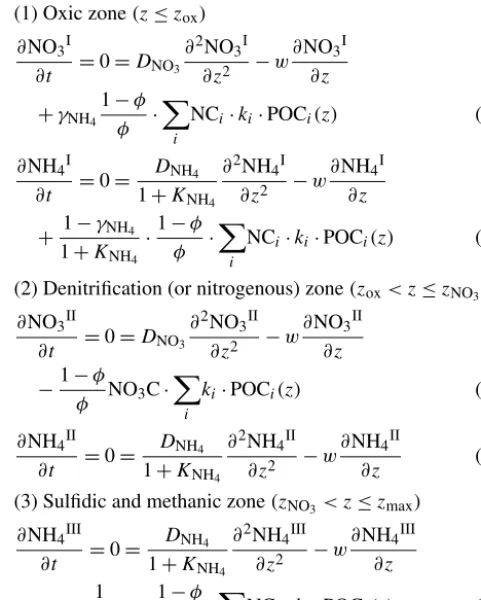
Figure 1.Schematic of the different modelled species and zones in OMEN-SED. Here the casezox< zbio< zNO3< zSO4 is shown.
2.1 General model approach
In OMEN-SED, the calculation of benthic uptake, recycling and burial fluxes is based on the vertically resolved conserva-tion equaconserva-tion for solid and dissolved species in porous media (e.g. Berner, 1980; Boudreau, 1997):
ξ∂Ci
∂t = −
∂
∂z
−ξ Di
∂Ci
∂z +ξ wCi
+ξX
j
Rji, (1)
whereCi is the concentration of biogeochemical species i,
and ξ equals the porosity φ for solute species and(1−φ)
for solid species. The termzis the sediment depth,tdenotes the time,Diis the apparent diffusion coefficient of speciesi,
wis the advection rate andP jR
j
i represents the sum of all
biogeochemical ratesj affecting speciesi.
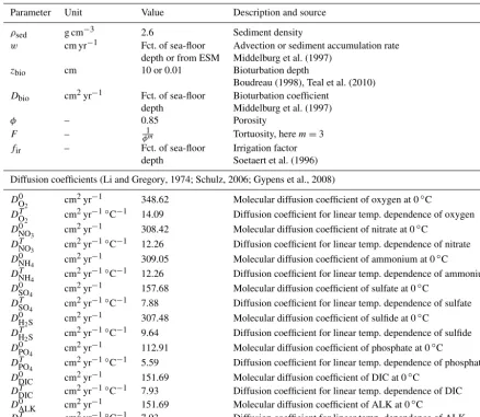
OMEN-SED accounts for both the advective and the dif-fusive transport of solid and dissolved species. They are buried in the sediment according to a constant advection rate w, thus neglecting the effect of sediment compaction (i.e. ∂φ∂z =0) due to mathematical constraints. The molec-ular diffusion of dissolved species is described by Fick’s law applying a species-specific apparent diffusion coeffi-cient,Dmol,i. In addition, the activity of infaunal organisms
in the bioturbated zone is simulated using a diffusive term (e.g. Boudreau, 1986), with a constant bioturbation coeffi-cientDbioin the bioturbated zone, whileDbiois set to zero below the maximum bioturbation depth,zbio. The pumping
activity by burrow-dwelling animals and the resulting venti-lation of tubes, the so-called bio-irrigation, is encapsulated in a factorfirthat enhances the molecular diffusion coefficient
(hence,Di,0=Dmol,i·fir; Soetaert et al., 1996). The reaction
network of OMEN-SED accounts for the most important pri-mary and secondary redox reactions, equilibrium reactions,
mineral dissolution and precipitation, and the adsorption and desorption processes associated with OM dynamics that af-fect the dissolved and solid species explicitly resolved in the model. Tables 1 and A1 provide a summary of the reactions and biogeochemical tracers considered in OMEN-SED to-gether with their respective reaction stoichiometries.
All parameters in Eq. (1), apart from porosity and burial rate, may vary with sediment depth and many reaction rate expressions depend on the concentration of other species. Expressing Eq. (1) for a set of chemical species thus re-sults in a non-linear, coupled set of equations that can only be solved numerically. However, OMEN-SED is designed for coupling to Earth system models and therefore cannot afford a computationally expensive numerical solution. In-stead, similar to early analytical diagenetic models, a com-putationally efficient analytical solution to Eq. (1) can be de-rived by (1) assuming steady-state conditions (i.e.∂Ci
∂t =0)
and (2) reducing the vertical variability in parameters and re-action rate expressions by dividing the sediment column into a number of functional biogeochemical zones (Fig. 1; com-pare e.g. Billen, 1982; Goloway and Bender, 1982; Ruardij and Van Raaphorst, 1995; Tromp et al., 1995; Gypens et al., 2008, for similar solutions). More specifically, OMEN-SED follows Berner (1980) by dividing the sediment column into (I) a bioturbated and (II) a non-bioturbated zone defined by an imposed, constant bioturbation depthzbio (Fig. 1).
Fur-thermore, it resolves the dynamic redox stratification of ma-rine sediments by dividing the sediment into (1) an oxic zone delineated by the oxygen penetration depthzox; (2) a denitrification (or nitrogenous) zone situated between zox
and the nitrate penetration depthzNO3; (3) a sulfate reduc-tion zone situated betweenzNO3 and the sulfate penetration depthzSO4; and (4) a methanogenic zone situated belowzSO4
(Fig. 1). Although in each of these zones Eq. (1) is applied with depth invariant parameters, parameter values may dif-fer across zones. The biogeochemical zones are linked by stating continuity in both concentrations and fluxes at the dy-namic, internal boundaries (zb∈ {zbio, zox, zNO3, zSO4};
com-pare e.g. Billen, 1982; Ruardij and Van Raaphorst, 1995). Note that these boundaries are dynamic because their depth varies in response to changing ocean boundary conditions and forcings (see Sect. 2.3.1 for details). Furthermore, the maximum bioturbation depth is not restricted to a specific biogeochemical zone, and hence OMEN-SED allows biotur-bation to occur in the anoxic zones of the sediment (here all zonesz > zoxcombined).
Table 1. Reactions and biogeochemical tracers implemented in the reaction network of OMEN-SED. The primary and secondary redox reactions are listed in the sequence they occur with increasing sediment depth.
Description
Primary redox reactions Degradation of organic matter via aerobic degradation, denitrification, sulfate reduction,
methanogenesis (implicit)
Secondary redox reactions Oxidation of ammonium and sulfide by oxygen, anaerobic oxidation of methane by sulfate
Adsorption and desorption Adsorption and desorption of P on or from Fe(OH)3, NH4adsorption, PO4adsorption
Mineral precipitation Formation of authigenic P, pyrite precipitation (implicit)
Biogeochemical tracers Organic matter (2G or pseudo 3G), oxygen, nitrate, ammonium, sulfate, sulfide (hydrogen sulfide),
phosphate, Fe-bound P, DIC, ALK
matter are a function of the organic matter concentration. Because organic matter degradation is described as a first-order degradation, these processes can be expressed as a se-ries of exponential terms (P
jαjexp(−βjz); see Eq. 2). In
addition, slow adsorption and desorption and mineral pre-cipitation processes can be expressed as zero- or first-order (reversible) reactions (Qmor kl·Ci in Eq. 2). Fast
adsorp-tion is described as an instantaneous equilibrium reacadsorp-tion us-ing a constant adsorption coefficientKi. The reoxidation of
reduced substances is accounted for implicitly by adding a (consumption and production) flux to the internal boundary conditions (see Sect. 2.2.2, 2.2.3 and 2.2.4). This simplifica-tion has been used previously by Gypens et al. (2008) for nitrate and ammonium and can be justified as it has been shown that reoxidation mainly occurs within a thin layer at the oxic–anoxic interface (Soetaert et al., 1996). The general reaction–transport equation underlying OMEN-SED is thus given by
∂Ci
∂t =0=
Di
1+Ki
∂2Ci
∂z2 −w ∂Ci
∂z −
1 1+Ki X
j
αjexp(−βjz)+ X
l
kl·Ci− X
m
Qm !
, (2)
where 1/βj can be interpreted as the length scale andαj
as the relative importance (or the magnitude at z=0) of reactionj(Boudreau, 1997);klrepresents generic first-order
reaction rate constants and Qm represents zero-order (or
constant) reaction rates.
The analytical solution to Eq. (2) is of the general form
Ci(z)=A·exp(az)+B·exp(bz)+ X
j
αj
Dβj2−wβj−Plkl
·exp(−βjz)+ P
mQm P
lkl
, (3)
with
a=
w−
q
w2+4·D·P lkl
2·D ,
b=
w+
q
w2+4·D·P lkl
2·D (4)
whereAandB are integration constants that can be deter-mined by applying a set of internal boundary conditions (see Sect. 2.3) andD= Di
1+Ki.
Based on Eq. (2) and its analytical solution Eq. (3), OMEN-SED returns the fraction of particulate organic car-bon (POC) buried in the sediment, fPOC, and the benthic uptake and return fluxes FCi of dissolved species Ci (in
mol cm−2yr−1) in response to the dynamic interplay of transport and reaction processes under changing boundary conditions and forcings:
fPOC=POC(zmax)
POC(0) , (5)
FCi=φ (0)
Di
∂Ci(z)
∂z
z=0
−w·Ci(0)
, (6)
wherewis the deposition rate,Di is the diffusion coefficient
and POC(0), POC(zmax)andCi(0)denote the concentration
of POC and dissolved speciesiat the sediment–water inter-face (SWI) and at the lower sediment boundary, respectively. 2.2 Conservation equations and analytical solution The following sections provide a detailed description of the conservation equations and analytical solutions for each chemical species that is resolved in this version of OMEN-SED.
2.2.1 Organic matter or particulate organic carbon (POC)
In marine sediments, organic matter (or in the following called particulate organic carbon, POC) is degraded by het-erotrophic activity coupled to the sequential utilisation of ter-minal electron acceptors (TEAs) according to the free energy gain of the half-reaction (O2>NO−3 >MnO2>Fe(OH)3>
into a numberiof discrete compound classes POCi
charac-terised by class-specific first-order degradation rate constants
ki. The conservation equation for organic matter dynamics is
thus given by
∂POCi
∂t =0=DPOCi ∂2POCi
∂z2 −w
∂POCi
∂z −ki·POCi, (7)
withDPOCi=Dbioforz≤zbioandDPOCi=0 forz > zbio. Integration of Eq. (7) yields the following general solutions for the bioturbated and non-bioturbated layers.
(I) Bioturbated zone(z≤zbio)
POCIi(z)=A1i·exp(a1iz)+B1i·exp(b1iz) (8)
(II) Non-bioturbated zone(zbio< z)
POCIIi(z)=A2i·exp(a2iz) (9)
In the above equations,
a1i=
w−pw2+4·DPOC
i·ki
2·DPOCi , b1i=
w+pw2+4·D POCi·ki
2·DPOCi
, a2i= −
ki
w. (10)
Determining the integration constants (A1,i, B1,i, A2,i)
re-quires the definition of a set of boundary conditions (Table 2). For organic matter, OMEN-SED applies a known concen-tration at the sediment–water interface and assumes conti-nuity across the bottom of the bioturbated zone,zbio. When OMEN-SED is coupled to an ESM, the POC depositional flux from the coupled ocean model is converted to a con-centration by solving the flux divergence Eq. (51). The in-tegration constants (A1,i, B1,i, A2,i) are thus given by the
following.
B1i
BC1)
= POC0i−A1i (11)
A2i
BC2)
= A1i·exp(a1iz −
bio)+B1i·exp(b1iz − bio)
exp(a2iz+bio)
A1i
BC3)
= −B1ib1i·exp(b1iz − bio) a1i·exp(a1izbio− )
See Sect. 2.3.1 for further details on how to find the analytical solution.
2.2.2 Oxygen
OMEN-SED explicitly accounts for oxygen consumption by the aerobic degradation of organic matter within the oxic zone and the oxidation of reduced species (i.e. NH4, H2S)
produced in the anoxic zones of the sediment. In the oxic zone (z < zox), aerobic degradation consumes oxygen with
a fixed O2:C ratio (O2C, Table 10). A predefined
frac-tion, γNH4, of the ammonium produced during the aerobic
degradation of OM is nitrified to nitrate, consuming 2 moles
of oxygen per mole of ammonium produced. In addition, OMEN-SED implicitly accounts for oxygen consumption due to the oxidation of reduced species (NH4, H2S) produced
below the oxic zone through the flux boundary condition at the dynamically calculated oxygen penetration depthzox(see
Sect. 2.4.2 for details). All oxygen consumption processes can thus be formulated as a function of organic matter degra-dation. The conservation equation for oxygen is given by
∂O2
∂t =0=DO2 ∂2O2
∂z2 −w ∂O2
∂z −
1−φ φ
X
i
ki
· [O2C+2γNH4NCi] ·POCi(z). (12)
For illustrative purposes, we here substitute the analytical so-lution for the POC depth profile and provide the analytical solution. The remaining paragraphs only outline the general equation, whose analytical solution can be derived in an iden-tical manner. Substituting Eqs. (8) and (9) for POCi(z) and
Eq. (11) forB1i gives the following.
(I) Bioturbated zone(z≤zbio) ∂OI2
∂t =0
8&11
= DIO
2
∂2O2 ∂z2 −w
∂O2
∂z −
1−φ φ
X
i
ki
· [O2C+2γNH4NCi] · A1i· [exp(a1iz)−exp(b1iz)]
+POC0i·exp(b1iz)
(II) Non-bioturbated zone(zbio< z < zox) ∂O2II
∂t =0
9
=DIIO
2
∂2O2 ∂z2 −w
∂O2
∂z −
1−φ φ
X
i
ki
· [O2C+2γNH4NCi] · A2i·exp(a2iz)
DIO
2andD
II
O2denote the O2diffusion coefficient for the
bio-turbated and non-biobio-turbated zone, respectively. The term
1−φ
φ accounts for the volume conversion from solid to
dis-solved phase and NCiis the nitrogen to carbon ratio in POC.
Integration yields the following analytical solution for each zone.
(I) Bioturbated zone(z≤zbio): O2I(z)=A1O2+B
1 O2·exp(b
1 O2z)+
X
i
8I1,i·exp(a1iz)
+X
i
8II1,i·exp(b1iz)+ X
i
8III1,i·exp(b1iz) (13)
(II) Non-bioturbated zone(zbio< z < zox)
O2II(z)=A2O2+B
2
O2·exp(b
2 O2z)
+X
i
8Ii,2·exp(a2iz) (14)
with
b1O
2 =
w
DOI
2
, bO2
2=
w
DIIO
2
8I1,i=1−φ
φ ·
ki·(O2C+2γNH4NCi)·A1i
DOI
2(−a1i)
2−w·(−a1
i)
Table 2.OM Boundary conditions applied in OMEN-SED. For the boundaries we definez−bio=limh→0(zbio−h)andz+bio=limh→0(zbio+
h).
Boundary Condition
z=0 Known concentration (1) POCi(0)=POC0i
z=zbio Continuity (2) POCi(zbio− )=POCi(z+bio)
(3) −Dbio·∂POC∂z i|z−bio=0
8II1,i= −1−φ
φ ·
ki·(O2C+2γNH4NCi)·A1i
DOI
2(−b1i)
2−w·(−b1
i)
8III1,i=1−φ
φ ·
ki·(O2C+2γNH4NCi)·POC0i
DOI
2(−b1i)
2−w·(−b 1i)
8Ii,2:=1−φ
φ ·
ki·(O2C+2γNH4NCi)·A2i
DIIO
2(−a2i)
2−w·(−a 2i)
Determining the four integration constants (A1O
2, B
1 O2, A
2 O2, B
2
O2; see Sect. 2.3 for details) and the
a priori unknown oxygen penetration depth requires the definition of five boundary conditions (see Table 3). At the sediment–water interface, OMEN-SED applies a Dirichlet condition (i.e. known concentration) and assumes con-centration and flux continuity across the bottom of the bioturbated zone, zbio. The oxygen penetration depth zox
marks the lower boundary and is dynamically calculated as the depth at which O2(z)=0. Therefore, OMEN-SED applies a Dirichlet boundary condition O2(zox)=0. In addition, a flux boundary is applied that implicitly accounts for the oxygen consumption by the partial oxidation of NH4
and H2S diffusing into the oxic zone from below (BC 4.2;
Table 3). It is assumed that respective fractions (γNH4 and
γH2S) are directly reoxidised at the oxic–anoxic interface and
the remaining fraction escapes reoxidation (or is precipitated as pyrite, γFeS). OMEN-SED iteratively solves for zox by
first testing if there is oxygen left atzmax(i.e. O2(zmax) >0).
If that is not the case, it determines the root for the flux boundary condition 4.2 (Table 3). If zox=zmax, a zero
diffusive flux boundary condition is applied as a lower boundary condition.
2.2.3 Nitrate and ammonium
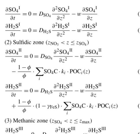
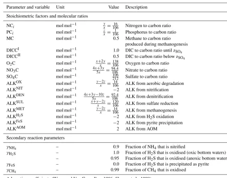
Nitrogen dynamics in OMEN-SED are controlled by the metabolic production of ammonium, nitrification, denitrifi-cation and ammonium adsorption. Ammonium is produced by organic matter degradation in both the oxic and anoxic zones, while denitrification consumes nitrate in the denitri-fication zone with a fixed NO3:C ratio (NO3C; Table 10).
Anaerobic ammonium oxidation (anammox) is implicitly in-cluded in the model. The organic nitrogen released during denitrification is assumed to be directly oxidised with nitrite to N2through a coupling between denitrification and
anam-mox.
The adsorption of ammonium to sediment particles is for-mulated as an equilibrium process with a constant equilib-rium adsorption coefficientKNH4, thus assuming that the
ad-sorption is fast compared to the characteristic timescales of transport processes (Wang and Van Cappellen, 1996). In ad-dition, a defined fraction,γNH4, of metabolically produced
ammonium is directly nitrified to nitrate in the oxic zone, while the nitrification of upward-diffusing ammonium pro-duced in the sulfidic and methanic zones is implicitly ac-counted for in the boundary conditions. The conservation equations for ammonium and nitrate are thus given by the following.
(1) Oxic zone(z≤zox) ∂NO3I
∂t =0=DNO3 ∂2NO3I
∂z2 −w
∂NO3I ∂z
+γNH41−φ
φ ·
X
i
NCi·ki·POCi(z) (15)
∂NH4I
∂t =0=
DNH4
1+KNH4
∂2NH4I
∂z2 −w
∂NH4I ∂z
+ 1−γNH4
1+KNH4
·1−φ
φ ·
X
i
NCi·ki·POCi(z) (16)
(2) Denitrification (or nitrogenous) zone(zox< z≤zNO3) ∂NO3II
∂t =0=DNO3
∂2NO3II
∂z2 −w
∂NO3II ∂z
−1−φ
φ NO3C·
X
i
ki·POCi(z) (17)
∂NH4II
∂t =0=
DNH4
1+KNH4
∂2NH4II
∂z2 −w
∂NH4II
∂z (18)
(3) Sulfidic and methanic zone(zNO3< z≤zmax) ∂NH4III
∂t =0=
DNH4
1+KNH4
∂2NH4III
∂z2 −w
∂NH4III ∂z
+ 1
1+KNH4 ·
1−φ
φ ·
X
i
NCi·ki·POCi(z) (19)
DNO3 andDNH4denote the diffusion coefficients for NO3
and NH4, which depend on the bioturbation status of the
Table 3.Boundary conditions for oxygen. For the boundaries we definezbio− =limh→0(zbio−h)andz+bio=limh→0(zbio+h).
Boundary Condition
z=0 Known concentration (1) O2(0)=O20
z=zbio Continuity (2) O2(z−bio)=O2(z+bio)
(3) − DO2,0+Dbio
·∂O2
∂z |z−bio= −DO2,0· ∂O2
∂z |z+bio
z=zox O2consumption (4) IF(O2(zmax) >0)
(zox=zmax) (4.1) ∂∂zO2|zox=0
ELSE
(zox< zmax) (4.2) O2(zox)=0 and −DO2· ∂O2
∂z |zox=Fred(zox)
with Fred(zox)=1−φφ·Rzmax
ezNO3 P
i 2γNH4NCi+2γH2S(1−γFeS)SO4C
kiPOCi dz
Note:ezNO3=zoxas the upper boundary here, aszNO3is not known at this point.
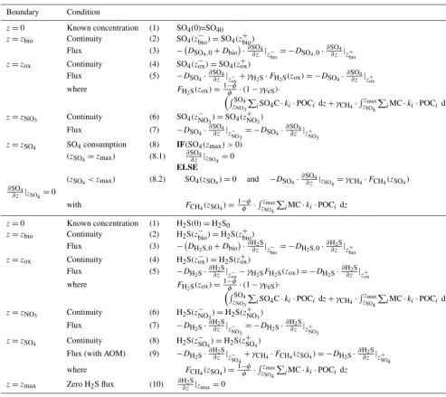
details on how to find the analytical solution). Table 4 sum-marises the boundary conditions applied in OMEN-SED to solve Eqs. (15)–(19) and to find the a priori unknown nitrate penetration depth,zNO3. The model assumes known bottom
water concentrations for both NO3and NH4, the complete
consumption of nitrate at the nitrate penetration depth (in the casezNO3< zmax) and no change in ammonium flux atzmax.
In addition, concentration and diffusive flux continuity across
zbioandzoxis considered for NO3and NH4. Furthermore, the
reoxidation of upward-diffusing reduced ammonium is ac-counted for in the oxic–anoxic boundary condition for nitrate and ammonium. OMEN-SED iteratively solves forzNO3 by first testing if there is nitrate left atzmax(i.e. NO3(zmax) >0) and otherwise by finding the root for the flux boundary con-dition 6.2 (Table 4).
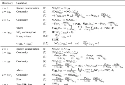
2.2.4 Sulfate and sulfide
Below the denitrification zone (z > zNO3), organic matter
degradation is coupled to sulfate reduction, consuming sul-fate and producing hydrogen sulfide with a fixed SO4:C
ra-tio (SO4C; Table 10). In addition, the anaerobic oxidation of
upward-diffusing methane (AOM) produced below the sul-fate penetration and the associated consumption of sulsul-fate and production of sulfide, as well as the production of sul-fate and consumption of sulfide through sulfide oxidation, are implicitly accounted for through the boundary conditions (Table 5). In the sulfidic zone a defined fraction of sulfide,
γFeS, can be precipitated as pyrite (in the presented simula-tionsγFeS=0.0 as we do not want to make any assumptions about pyrite precipitation). It can be safely assumed that al-most all CH4is oxidised anaerobically in the sediments (e.g.
Reeburgh, 2007, suggests up to 90 %), except for active (very localised) sites and slope failure, which can, in theory, be ac-counted for through the γCH4 term. The conservation
equa-tions for sulfate and sulfide are thus given by the following.
(1) Oxic and nitrogenous zone(z≤zNO3)
∂SO4I
∂t =0=DSO4 ∂2SO4I
∂z2 −w
∂SO4I
∂z (20)
∂H2SI
∂t =0=DH2S
∂2H2SI
∂z2 −w
∂H2SI
∂z (21)
(2) Sulfidic zone(zNO3< z≤zSO4)
∂SO4II
∂t =0=DSO4
∂2SO4II
∂z2 −w
∂SO4II ∂z
−1−φ
φ ·
X
i
SO4C·ki·POCi(z) (22)
∂H2SII
∂t =0=DH2S ∂2H2SII
∂z2 −w
∂H2SII ∂z
+1−φ
φ ·(1−γFeS)·
X
i
SO4C·ki·POCi(z) (23)
(3) Methanic zone(zSO4< z≤zmax) ∂H2SIII
∂t =0=DH2S
∂2H2SIII
∂z2 −w
∂H2SIII
∂z (24)
DSO4andDH2Sdenote the diffusion coefficients for SO4and
H2S, which depend on the bioturbation status of the
respec-tive geochemical zone (compare to Sect. 2.3.1). Integration of Eqs. (20)–(24) yields the analytical solution and Table 5 summarises the boundary conditions applied. OMEN-SED assumes known concentrations at the sediment–water inter-face and continuity across the bioturbation depth and the ni-trate penetration depth. The reoxidation of reduced H2S to
SO4is accounted for implicitly via the oxic–anoxic
bound-ary condition for both species, while the reduction of SO4
and the associated production of H2S via AOM is accounted
for through the respective boundary conditions atzSO4. In the casezSO4< zmax, OMEN-SED assumes zero sulfate
concen-tration atzSO4 and its diffusive flux must equal the amount
of methane produced below (with a methane to carbon ra-tio of MC); in the case zSO4=zmax, a zero diffusive flux
condition for sulfate is considered. OMEN-SED iteratively solves forzSO4 by first testing if there is sulfate left atzmax
Table 4.Boundary conditions for nitrate and ammonium. For the boundaries we definez−__=limh→0(z__−h)andz+__=limh→0(z__+h).
Boundary Condition
z=0 Known concentration (1) NO3(0)=NO30
z=zbio Continuity (2) NO3(z−bio)=NO3(z+bio)
(3) − DNO3,0+Dbio
·∂NO3
∂z |z−bio= −DNO3,0·∂NO∂z3|z+bio
z=zox Continuity (4) NO3(z−ox)=NO3(z+ox)
(5) −DNO3·∂NO3
∂z |z−ox+γNH4·FNH4(zox)= −DNO3· ∂NO3
∂z |z+ox
where FNH4(zox)=
1 1+KNH4 ·
1−φ
φ ·
Rzmax
zNO3
P
iNCi·ki·POCi dz
z=zNO3 NO3consumption (6) IF(NO3(zmax) >0)
(zNO3=zmax) (6.1)
∂NO3
∂z |zNO3 =0 ELSE
(zNO3< zmax) (6.2) NO3(zNO3)=0 and ∂NO3
∂z |zNO3 =0
z=0 Known concentration (1) NH4(0)=NH40
z=zbio Continuity (2) NH4(z−bio)=NH4(z+bio)
(3) −DNH4,0+Dbio 1+KNH4 ·
∂NH4
∂z |z−bio= − DNH4,0
1+KNH4 · ∂NH4
∂z |z+bio
z=zox Continuity (4) NH4(z−ox)=NH4(z+ox)
(5) − DNH4
1+KNH4 · ∂NH4
∂z |z−ox−γNH4·FNH4(zox)= − DNH4
1+KNH4 · ∂NH4
∂z |z+ox
where FNH4(zox)=
1 1+KNH4 ·
1−φ
φ ·
Rzmax zNO3
P
iNCi·ki·POCi dz
z=zNO3 Continuity (6) NH4(z
−
NO3)=NH4(z
+ NO3)
Flux (7) − DNH4
1+KNH4 · ∂NH4
∂z |z− NO3
= − DNH4 1+KNH4·
∂NH4 ∂z |z+
NO3
z=zmax Zero NH4flux (8) ∂NH∂z4|zmax=0
flux boundary condition 8.2 (Table 5). At the lower boundary
zmaxzero diffusive flux of H2S is considered.
2.2.5 Phosphate
The biogeochemical description of phosphorus (P) dynamics builds on earlier models developed by Slomp et al. (1996) and accounts for phosphorus recycling through organic mat-ter degradation, adsorption onto sediments and iron(III) hy-droxides (Fe-bound P), as well as carbonate fluorapatite (CFA or authigenic P) formation (see Fig. 2 for a schematic overview of the sedimentary P cycle). In the oxic zone of the sediment, PO4 liberated through organic matter
degra-dation can adsorb to iron(III) hydroxides forming Fe-bound P (or FeP; Slomp et al., 1998). Below the oxic zone, PO4
is not only produced via organic matter degradation but can also be released from the Fe-bound P pool due to the reduc-tion of iron(III) hydroxides under anoxic condireduc-tions. Further-more, in these zones phosphate concentrations build up and pore waters can thus become supersaturated with respect to carbonate fluorapatite, thus triggering the authigenic forma-tion of CFA (Van Cappellen and Berner, 1988). Phosphorus bound in these authigenic minerals represents a permanent sink for reactive phosphorus (Slomp et al., 1996). As for am-monium, the adsorption of P to the sediment matrix is treated as an equilibrium process parameterised with dimensionless adsorption coefficients for the oxic and anoxic zone,
respec-PO4 Organic M
Fe-bound P Organic M
Authigenic P
Fe-bound P Organic M
Water column
Oxic sediments
Anoxic sediments PO4
PO4 ki
ki
ki
ks
km ka pi
Figure 2.A schematic of the sedimentary P cycle in OMEN-SED. Red numbers represent kinetic rate constants for phosphorus dy-namics (compare to Table 10;pi represents the uptake rate of PO4
via primary production in shallow environments). Adapted from Slomp et al. (1996).
tively (KPOox
4,K
anox
PO4 ; Slomp et al., 1998). The adsorption and
Table 5.Boundary conditions for sulfate and sulfide. For the boundaries we definez−__=limh→0(z__−h)andz+__=limh→0(z__+h).
Boundary Condition
z=0 Known concentration (1) SO4(0)=SO40
z=zbio Continuity (2) SO4(z−bio)=SO4(z+bio)
Flux (3) − DSO4,0+Dbio
·∂SO4
∂z |zbio− = −DSO4,0·∂SO∂z4|z+bio
z=zox Continuity (4) SO4(z−ox)=SO4(z+ox)
Flux (5) −DSO4·
∂SO4
∂z |z−ox+γH2S·FH2S(zox)= −DSO4· ∂SO4
∂z |z+ox
where FH2S(zox)=
1−φ
φ ·(1−γFeS)·
RSO4
zNO3
P
iSO4C·ki·POCi dz+γCH4·
Rzmax
zSO4
P
iMC·ki·POCi dz
z=zNO3 Continuity (6) SO4(z
−
NO3)=SO4(z
+ NO3)
Flux (7) −DSO4·
∂SO4 ∂z |z−
NO3
= −DSO4· ∂SO4
∂z |z+ NO3
z=zSO4 SO4consumption (8) IF(SO4(zmax) >0)
(zSO4=zmax) (8.1)
∂SO4
∂z |zSO4=0 ELSE
(zSO4< zmax) (8.2) SO4(zSO4)=0 and −DSO4· ∂SO4
∂z |zSO4=γCH4·FCH4(zSO4) ∂SO4
∂z |zSO4=0
with FCH4(zSO4)=
1−φ
φ ·
Rzmax
zSO4
P
iMC·ki·POCi dz
z=0 Known concentration (1) H2S(0)=H2S0
z=zbio Continuity (2) H2S(z−bio)=H2S(z+bio)
Flux (3) − DH2S,0+Dbio
·∂H2S
∂z |zbio− = −DH2S,0· ∂H2S
∂z |z+bio
z=zox Continuity (4) H2S(z−ox)=H2S(z+ox)
Flux (5) −DH2S·
∂H2S
∂z |z−ox−γH2SFH2S(zox)= −DH2S· ∂H2S
∂z |z+ox
where FH2S(zox)=
1−φ
φ ·(1−γFeS)·
RSO4
zNO3
P
iSO4C·ki·POCi dz+γCH4·
Rzmax zSO4
P
iMC·ki·POCi dz
z=zNO3 Continuity (6) H2S(z
−
NO3)=H2S(z
+ NO3)
Flux (7) −DH2S·
∂H2S ∂z |z−
NO3
= −DH2S· ∂H2S
∂z |z+ NO3
z=zSO4 Continuity (8) H2S(z
−
SO4)=H2S(z
+ SO4)
Flux (with AOM) (9) −DH2S·∂H2S
∂z |z− SO4
+γCH4·FCH4(zSO4)= −DH2S·∂H2S ∂z |z+
SO4
where FCH4(zSO4)=
1−φ
φ ·
Rzmax zSO4
P
iMC·ki·POCi dz
z=zmax Zero H2S flux (10) ∂H∂z2S|zmax=0
of the respective process is calculated as the product of the rate constant and the difference between the current concen-tration (of PO4 and FeP) and an equilibrium or asymptotic
concentration (Slomp et al., 1996). The asymptotic Fe-bound P concentration is FeP∞and the equilibrium concentrations for P sorption and authigenic fluorapatite formation are PO4s
and PO4a, respectively (Table 10). The last term in Eqs. (25)
and (26) represents the sorption of PO4 to FeP in the oxic
zone, the last term in Eqs. (27) and (28) is the release of PO4
from the FeP pool and the fourth term in Eq. (28) represents the permanent loss of PO4to authigenic fluorapatite
forma-tion. The conservation equations for phosphate and Fe-bound P are thus given by the following.
(1) Oxic zone(z≤zox)
∂PO4I
∂t =
DPO4
1+KPOox
4
∂2PO4I
∂z2 −w
∂PO4I ∂z
+1−φ
φ
1 1+KPOox
4 X
i
(PCi·ki·POCi(z))
− ks 1+KPOox
4
(PO4I−PO4s) (25)
∂FePI
∂t =DFeP
∂2FePI
∂z2 −w
∂FePI
∂z
+ φ
1−φks(PO4 I−PO
4s) (26)
(2) Anoxic zones(zox< z≤zmax) ∂FePII
∂t =DFeP
∂2FePII
∂z2 −w
∂FePII
−km(FePII−FeP∞) (27)
∂PO4II
∂t =
DPO4
1+KPOanox
4
∂2PO4II
∂z2 −w
∂PO4II ∂z
+1−φ
φ
1 1+KPOanox
4 X
i
(PCi·ki·POCi(z))
− ka 1+KPOanox
4
(PO4II−PO4a)
+(1−φ)
φ
km
1+KPOanox
4
(FePII−FeP∞) (28)
DPO4 denotes the diffusion coefficient for PO4, which
de-pends on the bioturbation status of the respective geochem-ical zone, and DFeP=Dbio for z≤zbio and DFeP=0 for z > zbio (compare to Sect. 2.3.1). Integration of Eqs. (25)–
(28) yields the analytical solution and Table 6 summarises the boundary conditions applied in OMEN-SED. The model as-sumes known bottom water concentrations and equal concen-trations and diffusive fluxes atzbioandzoxfor both species.
Additionally, OMEN-SED considers no change in phosphate flux and an asymptotic Fe-bound P concentration atzmax. 2.2.6 Dissolved inorganic carbon (DIC)
OMEN-SED accounts for the production of dissolved inor-ganic carbon (DIC) through orinor-ganic matter degradation and methane oxidation. Organic matter degradation produces dis-solved inorganic carbon with a stoichiometric DIC:C ratio of 1:2 in the methanic zone and 1:1 in the rest of the sed-iment column (DICCIIand DICCI, respectively). DIC pro-duction through methane oxidation is implicitly taken into account through the boundary condition at zSO4. A
mecha-nistic description of DIC production from CaCO3
dissolu-tion would lead to significant mathematical problems and is therefore not included in the current version of OMEN-SED. The conservation equations for DIC are thus given by the following.
(1) Oxic, nitrogenous and sulfidic zone(z≤zSO4)
∂DICI
∂t =0=DDIC
∂2DICI
∂z2 −w
∂DICI
∂z +
1−φ φ
·X
i
DICCI·ki·POCi(z) (29)
(2) Methanic zone(zSO4< z≤zmax)
∂DICII
∂t =0=DDIC
∂2DICII
∂z2 −w
∂DICII
∂z +
1−φ φ
·X
i
DICCII·ki·POCi(z) (30)
DDIC denotes the diffusion coefficient for DIC (taking the
values for HCO−3 from Schulz, 2006), which depends on the bioturbation status of the respective geochemical zone. In-tegration of Eqs. (29) and (30) yields the analytical solu-tion and Table 7 summarises the boundary condisolu-tions
ap-plied in OMEN-SED. A Dirichlet condition is apap-plied at the sediment–water interface. In addition, the model assumes a zero diffusive flux through the lower boundaryzmaxand con-tinuity across the bottom of the bioturbated zone and the sul-fate penetration depth. An additional flux boundary condition atzSO4 implicitly accounts for DIC production through the
anaerobic oxidation of methane (Table 7 Eq. 5). 2.2.7 Alkalinity
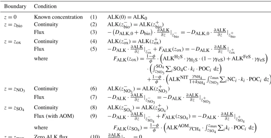
Organic matter degradation and secondary redox reactions exert a complex influence on alkalinity (e.g. Jourabchi et al., 2005; Wolf-Gladrow et al., 2007; Krumins et al., 2013). To model alkalinity, OMEN-SED divides the sediment column into four geochemical zones in which different equations de-scribe the biogeochemical processes using variable stoichio-metric coefficients (compare values in Table 10). Abovezox,
the combined effects of NH4 and P release due to aerobic
OM degradation increases alkalinity according to ALKOX, whereas nitrification decreases alkalinity with stoichiometry ALKNIT. In the remaining three zones anaerobic OM degra-dation generally results in an increase in alkalinity, with the exact magnitude depending on the nature of the terminal electron acceptor used (i.e. ALKDEN, ALKSUL, ALKMET). In addition, the effect of secondary redox reactions, such as nitrification, sulfide and methane oxidation, and pyrite pre-cipitation are implicitly accounted for in the boundary con-ditions. Note that the alkalinity description in the current ver-sion of OMEN-SED does not account for CaCO3dissolution
and precipitation due to the mathematical complexity of the problem. In OMEN-SED, the conservation equations for al-kalinity are thus given by the following.
(1) Oxic zone(z≤zox) ∂ALKI
∂t =0=DALK
∂2ALKI
∂z2 −w
∂ALKI
∂z
+1−φ
φ ·
X
i
ALKNIT· γNH4 1+KNH4
NCi+ALKOX
·ki·POCi(z) (31)
(2) Denitrification or nitrogenous zone(zox< z≤zNO3)
∂ALKII
∂t =0=DALK
∂2ALKII
∂z2 −w
∂ALKII
∂z
+1−φ
φ ·
X
i
ALKDEN·ki·POCi(z) (32)
(3) Sulfidic zone(zNO3< z≤zSO4)
∂ALKIII
∂t =0=DALK
∂2ALKIII
∂z2 −w
∂ALKIII
∂z
+1−φ
φ ·
X
i
ALKSUL·ki·POCi(z) (33)
Table 6. Boundary conditions for phosphate and Fe-bound P (FeP). For the boundaries we definez−__=limh→0(z__−h)and z+__=
limh→0(z__+h).
Boundary Condition
z=0 Known concentration (1) PO4(0)=PO40
z=zbio Continuity (2) PO4(zbio− )=PO4(z+bio)
Flux (3) DPO4,0+Dbio
·∂PO4
∂z |z−bio=DPO4,0·∂PO∂z4|z+bio
z=zox Continuity (4) PO4(zox−)=PO4(z+ox)
Flux (5)− DPO4
1+Kox PO4
·∂PO4 ∂z |z−ox= −
DPO4
1+Kanox PO4
·∂PO4 ∂z |z+ox
z=zmax Flux (10) ∂PO∂z4|zmax=0
z=0 Known concentration (1) FeP(0)=FeP0
z=zbio Continuity (2) FeP(z−bio)=FeP(z
+ bio)
Flux (3)∂FeP∂z |
z−bio= ∂FeP
∂z |z+bio
z=zox Continuity (4) FeP(z−ox)=FeP(z+ox)
Flux (5)∂FeP∂z |
z−ox= ∂FeP
∂z |z+ox
z=zmax Asymptotic concentration (10) FeP(zmax)=FeP∞
Table 7.Boundary conditions for DIC. For the boundaries we definez−__=limh→0(z__−h)andz+__=limh→0(z__+h).
Boundary Condition
z=0 Known concentration (1) DIC(0)=DIC0
z=zbio Continuity (2) DIC(z−bio)=DIC(z
+ bio)
Flux (3) − DDIC,0+Dbio·∂DIC∂z |z−
bio
= −DDIC,0·∂DIC∂z |z+
bio
z=zSO4 Continuity (4) DIC(z
−
SO4)=DIC(z
+ SO4)
Flux (with AOM) (5) −DDIC·∂DIC
∂z |z− SO4
+γCH4·FCH4(zSO4)= −DDIC·∂DIC
∂z |z+ SO4
where FCH4(zSO4)=
1−φ
φ ·
Rzmax zSO4
P
iMC·ki·POCi dz
z=zmax Zero DIC flux (6) ∂DIC∂z |zmax=0
∂ALKIV
∂t =0=DALK
∂2ALKIV
∂z2 −w
∂ALKIV
∂z
+1−φ
φ ·
X
i
ALKMET·ki·POCi(z) (34)
DALK denotes the diffusion coefficient for alkalinity (taking
the values for HCO−3 from Schulz, 2006), which depends on the bioturbation status of the respective geochemical zone. Integration of Eqs. (31)–(34) yields the analytical solution and Table 8 summarises the boundary conditions applied in OMEN-SED. A Dirichlet boundary condition is applied at the sediment–water interface. The decrease in alkalinity due to the oxidation of reduced species produced in the anoxic zones and due to the precipitation of pyrite (with stoichiom-etry ALKNIT, ALKH2S and ALKFeS) is implicitly taken into
account through the flux boundary condition atzox(Table 8 Eq. 5). Furthermore, the oxidation of methane by sulfate reduction increases alkalinity with stoichiometry ALKAOM, which is accounted for through the flux boundary condition atzSO4 (Table 8 Eq. 9). At the lower boundaryzmax a zero
diffusive flux condition is applied.
2.3 Determination of integration constants
The integration constants of all general analytical solutions derived above change in response to changing boundary conditions. Thus, OMEN-SED has to redetermine integra-tion constants for each dynamic zone (i.e.zox, zbio, zNO3 and
zSO4) at every time step for all biogeochemical species. The bioturbation boundary poses a particular challenge as it can theoretically occur in any of the dynamic geochemical zones (Fig. 3). Therefore, in order to generalise and simplify this re-curring boundary matching problem, an independent, generic algorithm (generic boundary condition matching) is imple-mented (rather than using multiple fully-worked-out alge-braic solutions for each possible case and every biogeochem-ical species). As a consequence, the algorithm only has to solve a two-simultaneous-equation problem.
Table 8.Boundary conditions for alkalinity. For the boundaries we definez−__=limh→0(z__−h)andz+__=limh→0(z__+h).
Boundary Condition
z=0 Known concentration (1) ALK(0)=ALK0
z=zbio Continuity (2) ALK(z−bio)=ALK(zbio+ )
Flux (3) − DALK,0+Dbio·∂ALK∂z |z−
bio
= −DALK,0·∂ALK∂z |z+
bio
z=zox Continuity (4) ALK(z−ox)=ALK(z+ox)
Flux (5) −DALK·∂ALK∂z |z−ox+FALK(zox)= −DALK·
∂ALK
∂z |z+ox
where FALK(zox)=1−φφ·
ALKH2S·γ
H2S·(1−γFeS)+ALK
FeS·γ FeS
·
RSO4 zNO3
P
iSO4C·ki·POCi dz
+1−φ
φ ·
ALKNIT1+γNH4k NH4
Rzmax zNO3
P
iNCi·ki·POCi dz
z=zNO3 Continuity (6) ALK(z
−
NO3)=ALK(z
+ NO3)
Flux (7) −DALK·∂ALK∂z |z−
NO3
= −DALK·∂ALK∂z |z+
NO3
z=zSO4 Continuity (8) ALK(z
−
SO4)=ALK(z
+ SO4)
Flux (with AOM) (9) −DALK·∂ALK∂z |z−
SO4
+FALK(zSO4)= −DALK· ∂ALK
∂z |z+SO4
where FALK(zSO4)=
1−φ
φ ·
ALKAOMγCH4·
Rzmax
zSO4
P
iki·POCi dz
z=zmax Zero ALK flux (10) ∂ALK∂z |zmax=0
Cis of the general form
C(z)=A·exp(az)+B·exp(bz)+X
j
αj
Dβj2−wβj−k
·exp(−βjz)+
Q
k (35)
and can therefore be expressed as
C(z)=A·E(z)+B·F (z)+G(z), (36)
whereE(z)andF (z)are the homogeneous solutions to the ODE,G(z)the particular integral (collectively called the ba-sis functions), andAandBare the integration constants that must be determined using the boundary conditions (shown in Fig. 3 for the whole sediment column).
Each internal boundary matching problem (i.e. exclud-ing z=0 and z=zmax) involves matching continuity and
flux for the two solutions to the respective reaction–transport equation above (CU(z)“upper”) and below (CL(z)“lower”) the dynamic boundary atz=zb.
CU(z)=AU·EU(z)+BU·FU(z)+GU(z) (37)
CL(z)=AL·EL(z)+BL·FL(z)+GL(z) (38)
OMEN-SED generally applies concentration continuity and flux boundary conditions at its internal dynamic boundaries. Continuity (where for generality we allow a discontinuity
Vb):
CU(zb)=CL(zb)+Vb. (39)
Flux:
DUCU0(zb)+wCU(zb)=DLCL0(zb)+wCL(zb)+Fb, (40)
where w is advection, D represents the diffusion coeffi-cients andFb is any flux discontinuity (e.g. resulting from
secondary redox reactions). Considering that the advective flux above and below the boundary is equal (i.e.wCU(zb)=
wCL(zb)) and substituting the general ODE solutions (37)
and (38), the boundary conditions can be represented as two equations connecting the four integration constants:
EU FU
DUEU0 DUFU0 AU BU
=
EL FL
DLEL0 DLFL0 AL BL
+
GL−GU+Vb
DLG0L−DUG0U+Fb−wVb
, (41)
where the ODE solutionsE, F andG are all evaluated at
zb. Equation (41) can now be solved to giveAUandBU as
a function of the integration constants from the layer below (ALandBL), thereby constructing a piecewise solution for
both layers with just two integration constants (this is imple-mented in the functionbenthic_utils.matchsolnof OMEN-SED):
AU BU
=
c1 c2 c3 c4
AL BL
+
d1 d2
. (42)
Using Eq. (42), CU(z) in Eq. (37) can now be rewrit-ten as a function of AL and BL (implemented in ben-thic_utils.xformsoln):
CU(z)=(c1AL+c2BL+d1)·EU(z)+(c3AL+c4BL+d2)
·FU(z)+GU(z), (43)
and hence the “transformed” basis functions
EU∗(z), FU∗(z)andG∗U(z)can be defined such that
CU(z)=AL·E∗U(z)+BL·FU∗(z)+G ∗
Sediment column
zox
zbio
zNO3
zSO4
zmax Layer 1
Layer 2
Layer 3
Layer 4
Layer 5
A1, B1
E1(z), F1(z), G1(z)
A2, B2
E2(z), F2(z), G2(z)
A3, B3
E3(z), F3(z), G3(z)
A4, B4
E4(z), F4(z), G4(z)
A5, B5
E5(z), F5(z), G5(z)
Figure 3.Schematic of the generic boundary condition matching (GBCM) problem. Shown are the resulting integration constants (Ai, Bi) and ODE solutions (Ei, Fi, Gi) for the different sedi-ment layers and the bioturbation boundary (possible locations are indicated by the green vertical arrow).
where
E∗U(z)=c1EU(z)+c3FU(z)
FU∗(z)=c2EU(z)+c4FU(z) (45)
G∗U(z)=GU(z)+d1EU(z)+d2FU(z).
Equations (42), (44) and (45) can now be consecutively applied for each of the dynamic biogeochemical zone bound-aries (Fig. 3) starting at the bottom of the sediment column. The net result is a piecewise solution for the whole sediment column with just two integration constants (coming from the lowest layer), which can then be solved for by applying the boundary conditions at the sediment–water interface and the bottom of the sediments.
2.3.2 Abstracting out the bioturbation boundary The bioturbation boundary affects the diffusion coefficient of the modelled solutes and the conservation equation of or-ganic matter (and thereby the exact form of each reaction– transport equation). This boundary is particularly
inconve-nient as it can in principle occur in the middle of any of the dynamically shifting biogeochemical zones and therefore generate multiple cases (Fig. 3). The GBCM algorithm de-scribed above is thus not only used to construct a piecewise solution for the whole sediment column, but also to abstract out the bioturbation boundary. For each biogeochemical zone the “bioturbation status” is initially tested (i.e. fully bio-turbated, fully non-bioturbated or crossing the bioturbation boundary). Therefore, the upper and lower boundaries for the different zones (e.g. for the nitrogenous zonezU=zox,zL= zNO3) and the respective reactive terms and diffusion
coeffi-cients (bioturbated and non-bioturbated) are passed over to the routinezTOC.prepfg_l12in which the bioturbation sta-tus is determined. In the case that the bioturbation depth is located within this zone (i.e.zU< zbio< zL) a piecewise so-lution for this layer is constructed. Therefore, the reactive terms and diffusion coefficients are handed over to the rou-tineszTOC.calcfg_l1andzTOC.calcfg_l2, which calculate the basis functions (EU, FU, GU andEL, FL, GL) and their
derivatives for the bioturbated and the non-bioturbated part of this specific geochemical zone. The concentration and flux for both solutions atzbio are matched and the coefficients c1, c2, c3, c4, d1andd2(as in Eq. 42) are calculated by the
routinebenthic_utils.matchsoln. These coefficients and the “bioturbation status” of the layer are passed back to the main GBCM algorithm in which they can be used by the routine benthic_utils.xformsolnto calculate the “transformed” ba-sis functions (EU∗(z), FU∗(z), G∗U(z)) such that both layers are expressed in the same basis (compare Eqs. 43–45).
For instance, in the case of sulfate,zTOC.prepfg_l12is called three times before the actual profile is calculated (once per zone: oxic, nitrogenous, sulfidic) and hands back the in-formation about the “bioturbation status” of the three lay-ers and the coefficientsc1, c2, c3, c4, d1 andd2 for the
bio-geochemical zone including the bioturbation depth. When calculating the complete piecewise solution for the sedi-ment column, this information is passed to the function zTOC.calcfg_l12, which sorts out the correct solution type to use. The main GBCM algorithm therefore never needs to know whether it is dealing with a piecewise solution (i.e. matched across the bioturbation boundary) or a “sim-ple” solution (i.e. the layer is fully bioturbated or fully non-bioturbated).
2.4 Model parameters