Bayesian inference of earthquake rupture models using polynomial chaos expansion

(1)

Bayesian inference of earthquake rupture models using

polynomial chaos expansion

Hugo Cruz-Jiménez1_{, Guotu Li}2_{, Paul Martin Mai}1_{, Ibrahim Hoteit}1_{, and Omar M. Knio}1,2 1_{King Abdullah University of Science and Technology, Thuwal 23955, Saudi Arabia}

2_{Department of Mechanical Engineering and Materials Science, Duke University, Durham, NC 27708, USA} Correspondence:Guotu Li ([email protected]) and Omar M. Knio ([email protected])

Received: 8 January 2018 – Discussion started: 5 February 2018

Revised: 13 June 2018 – Accepted: 30 June 2018 – Published: 31 July 2018

Abstract. In this paper, we employed polynomial chaos (PC) expansions to understand earthquake rupture model re-sponses to random fault plane properties. A sensitivity anal-ysis based on our PC surrogate model suggests that the hypocenter location plays a dominant role in peak ground ve-locity (PGV) responses, while elliptical patch properties only show secondary impact. In addition, the PC surrogate model is utilized for Bayesian inference of the most likely underly-ing fault plane configuration in light of a set of PGV observa-tions from a ground-motion prediction equation (GMPE). A restricted sampling approach is also developed to incorporate additional physical constraints on the fault plane configura-tion and to increase the sampling efficiency.

1 Introduction

One of the most important challenges seismologists and earthquake engineers face in designing large civil structures (e.g., buildings, dams, bridges, power plants) and response plans, especially in highly populated cities prone to large damaging earthquakes, is the reliable estimation of ground-motion characteristics at a given location. Ground-ground-motion prediction equations (GMPEs), which are one of the most important elements for probabilistic seismic hazard analysis (PSHA), are designed for this purpose. These are obtained from regression analysis by fitting a dataset (empirical and simulated) and are mainly expressed in terms of site condi-tions, source–site distance (e.g., rupture distance or Joyner– Boore distance, denoted asR_JBdistance hereafter1), magni-1_{The Joyner–Boore distance is defined as the shortest distance}

from a site to the surface projection of the rupture plane.

tude, and mechanism, although other terms such as directiv-ity and hanging-wall effect are also considered (Abraham-son et al., 2014). The equations can be derived for peak ground displacement (PGD), peak ground velocity (PGV), peak ground acceleration (PGA), and spectral acceleration (SA) for a damping of 5 % at different periods. Ideally, an optimal GMPE has to be robust and include physical terms to avoid overfitting the data, which can result in the inclu-sion of too many parameters. When other effects are consid-ered (such as amplitude and duration of rupture directivity; Somerville et al., 1997) or more data are available (Atkin-son and Boore, 2011), GMPEs are modified to better explain attenuation patterns.

(2)

observed ground motion and GMPEs by including site ef-fects of the area. Numerical simulations have also helped to explain ground-motion characteristics. For instance, Fu-rumura and Singh (2002) described attenuation patterns for both deep in-slab and shallow interplate earthquakes, while Cruz-Jiménez et al. (2009) explained ground-motion ampli-fication due to a volcanic layer. Mahani and Atkinson (2012) modeled the decay of spectral amplitudes in several locations in North America.

In this study, we investigate the level of complexity needed in kinematic rupture models of magnitude 6.5 strike-slip events to produce ground motion similar to a reference GMPE. To this end, we utilize the polynomial chaos (PC) approach (Ghanem and Spanos, 1991; Xiu and Karniadakis, 2002; Le Maître and Knio, 2010) to build functional repre-sentations of PGV responses of an original source model. Thanks to the significant reduction in computational cost of the PC surrogate models (in comparison with both the orig-inal source model and a Bayesian analysis based on Markov chain Monte Carlo (MCMC) sampling, which requires a pro-hibitive number of model runs; Minson et al., 2014), it is suitable to utilize the PC surrogates in a Bayesian inference framework (Sudret and Mai, 2013; Sraj et al., 2016; Giraldi et al., 2017). This enables us to quantitatively rank different kinematic source models given by the PGVs they produce and identify the most likely one that fits a chosen reference GMPE (expectation). The ranking considers uncertainties in both the GMPE and model parameters. This provides useful insight on the level of complexity needed in kinematic source models for ground-motion simulations to satisfy both obser-vational constraints and engineering/design requirements for seismic safety.

This paper is organized as follows. In Sect. 2, we provide detailed descriptions of the source model configurations, in-cluding the calculation of synthetic seismograms. In Sect. 3, we present the PC analysis of PGVs as a function of random variations of the kinematic models, including the validation of PC surrogate models and discussions of various statistical quantities. In Sect. 4, we conduct a PC-based Bayesian in-ference analysis to identify the most likely kinematic rupture model that best fits a chosen GMPE reference curve. Finally, we conclude our key findings and propose potential improve-ments for future work in Sect. 5.

2 Source model

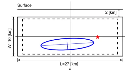
A magnitudeM_w=6.5 strike-slip earthquake (seismic mo-ment 6.31×1018Nm; rake=0◦) on a single-segment ver-tical fault plane is considered. The fault plane is chosen to be a rectangle with fixed length L=27 km and width W =10 km, which are the most frequent values among 100 sample realizations following scaling relations (e.g., Wells and Coppersmith, 1994; Mai and Beroza, 2000; Thingbaijam et al., 2017). The top of the fault plane is located 2 km below

2 [km]

X

Z Surface

L=27 [km]

W=10 [km]

Figure 1.Example of fault plane configuration. The red star denotes hypocenter location, and the ellipse is the asperity with Gaussian slip distribution inside. The slip distribution is tapered in the area between the dashed and solid rectangles.

the ground surface. Figure 1 shows an example configuration of the fault plane, in which the red star denotes the hypocen-ter and the ellipse is the asperity with Gaussian slip distri-bution inside. The maximum slipS_maxis chosen such that the mean slip (over the entire fault plane) remains constant (0.71 m) when varying the ellipse size (which ensures that the moment magnitude remains constant, M_w=6.5). The slip between the elliptical patch boundary and dashed rectangle (Fig. 1) is set to beS_max/e(wheree is the Euler number), the minimum value at the patch boundary from the Gaus-sian slip distribution. The slip between the solid and dashed rectangles (the horizontal and vertical gaps are 5 % of the length and width of the fault plane, respectively) is tapered to avoid non-physical slip patterns. The entire fault plane is dis-cretized in along-strike and down-dip directions with a grid size of 0.02 km. We use a regularized Yoffe function (Tinti et al., 2005) with a rise time Tr=1.25 s following source-scaling relations (Somerville et al., 1999) and slip accelera-tion timet_acc=0.225 s, as suggested by Tinti et al. (2005). At each node of the discretized fault plane, we assign Tr,t_acc, slip-rate in along-strike and down-dip directions, and rupture time. We consider a rupture speed of 0.75Vs(where the shear wave speedV_sis listed in Table 1) in all source models.

(3)

mini-Figure 2.A virtual network ofN_obs=56 stations where PGV

re-sponses are reported by the source model. The solid black line at the center denotes the length and location of the fault plane. Note that the 56 stations are grouped into four sets (indicated by differ-ent colors/symbols) according to theirR_JBdistances (see details in

Sect. 4).

Table 1.Velocity model used in this study, modified from Boore et al. (1997).

Depth (km) Vp(km s−1) Vs(km s−1)

0 2.4 1.5

0.5 4.4 2

1.5 5.3 2.7

2.5 5.5 2.9

4 5.7 3.3

8 6.1 3.5

14 6.8 3.9

16.6 7.1 4.1

27 8 4.6

350 8.2 4.65

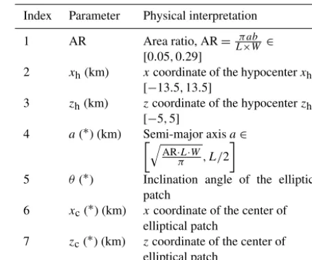
mum shear wavelength at depthz. The grid extends to a total depth that depends on the wavenumber, which means that the maximum depth decreases when the wavenumber increases. This approach considers a layered 1-D velocity structure. We apply the velocity model shown in Table 1, which corre-sponds to a slightly modified version of the generic model by Boore et al. (1997) for California. The resulting PGVs serve as our quantities of interest (QoIs, each denoted asQj, for j=1,2, . . ., N_obs). We aim at understanding stochastic source model PGV responses to random fault plane configu-rations of the source process (slip distributions and hypocen-ter location). To this end, we consider variations in seven physical parameters listed in Table 2, which parameterize the fault plane configurations, i.e., locations of both the hypocen-ter and elliptical asperity patch, as well as its shape and ori-entation. We restrict the hypocenter and elliptical patch to be inside the fault plane and limit the area ratio (AR) of the elliptical patch to the entire fault plane (L×W) between 5 and 29 %. These restrictions lead to nonlinear dependency between feasible ranges of different physical parameters (see Appendix A for more details).

Table 2.Parameters governing fault plane configurations.

Index Parameter Physical interpretation

1 AR Area ratio, AR= π ab

L×W ∈

[0.05,0.29]

2 x_h(km) xcoordinate of the hypocenterx_h∈

[−13.5,13.5_]

3 z_h(km) zcoordinate of the hypocenterz_h∈

[−5,5]

4 a(∗) (km) Semi-major axisa∈

q

AR·L·W π , L/2

5 θ(∗) Inclination angle of the elliptical

patch

6 x_c(∗) (km) xcoordinate of the center of

elliptical patch

7 zc(∗) (km) zcoordinate of the center of

elliptical patch

∗_{denotes parameters whose feasible ranges are dependent on others.}

3 Polynomial chaos framework

PC expansions (Ghanem and Spanos, 1991; Xiu and Kar-niadakis, 2002; Le Maître and Knio, 2010)2 _{are used in} this study to understand earthquake rupture model responses (in terms of PGVs) to random configurations of slip distri-bution and hypocenter location. We associate each of the physical parameters with a canonical PC random variableξi (i∈ {1,2, .. . ., n_d}, wheren_d=7 is the stochastic space di-mension) and assume allξi values are independent and uni-formly distributed over[−1,1]. That is, the joint distribution of the random parameter vectorξis

p(ξ)=

2−7 _if_ξ_∈₄_{≡ [−}_1,1_]7_,

0 otherwise. (1)

Each random parameter vector ξ∈4 can be linked

uniquely to a realization of the physical parameter vector (see mapping details in Appendix A). We thus focus on construct-ing functional representations of PGV responses at each sta-tion with respect to the canonical variableξ, which

param-eterize the physical parameters in Table 2. It is worth men-tioning that the mapping from canonical random variableξto

physical fault plane configuration parameters does not lead to uniform distributions for physical parameters, due to their in-terdependency as indicated in Table 2. Nevertheless, the va-lidity of PC expansions based on canonical random variable

ξis well maintained, as suggested by the cross-validation and

empirical error analyses later in this section.

Let Qj(ξ) be the PGV response to ξ at the jth station (j∈ {1,2, . . ., N_obs}), and assume eachQj is a second-order 2_{An open-source toolkit for the PC framework is available at}

(4)

random variable, i.e.,Qj(ξ)is in the Hilbert spaceL2(4, p), and

E h

Q2_ji₌ Z

4

Qj(ξ)2p(ξ)dξ<+∞, (2)

∀j∈ {1,2, . . ., N_obs}.

One can approximateQj(ξ)using a truncated PC expansion as follows:

Qj(ξ)≈Qej(ξ)= Np

X α₌0

cα9α(ξ), ∀j∈ {1,2, . . ., Nobs}, (3) whereN_pis a truncation parameter and(N_p+1)is the num-ber of expansion terms retained in the PC surrogate models. In this study, we truncated the PC expansion at total polyno-mial order ofq=9. Givenn_d=7, one can calculate the total number of polynomials via

Np+1=(q+nd)!

q!n_d! =11 440. (4)

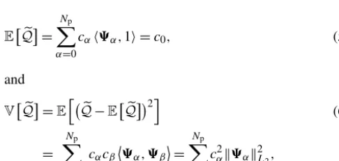
By adopting the classical convention of90(ξ)=1, the mean and variance of a PC surrogateQj(ξ)can be expressed as

EQe

=

Np

X α₌0

cαh9α,1i =c0, (5)

and VQe

=E h

e Q−EQe

2i

(6)

=

Np

X α,β=1

cαcβ9α,9β= Np

X α=1

c_α2k9αk2L2,

where _h·i denotes the inner product in the Hilbert space L₂(4, p) with respect to the joint distribution p(ξ) (Le Maître and Knio, 2010).

To determine the expansion coefficients (cα values) in Eq. (3), we rely on a Latin hypercube sample (LHS) (McKay et al., 1979) set (denoted asP_LHShereafter) ofN_LHS=8000 earthquake rupture model realizations through{ξ_k}₁_≤k_≤N_LHS, and solve the following basis pursuit denoising (BPDN) problem (Van Den Berg and Friedlander, 2007, 2008) 3 _at each station:

c∗=arg min

c_∈RNp+1

||c||l₁ s.t. ||Qj− [9]c|| ≤γ||Qj||l₂, (7)

∀j∈ {1,2, . . ., N_obs},

where Qj=(Qj(ξ₁),Qj(ξ₂), . . .,Qj(ξNLHS))T is the

model PGV realization vector at the jth station, and

c∈RNp+1is the coefficient vector for the corresponding PC 3_{The corresponding source code is available at https://github.}

com/mpf/spgl1 (last access: 20 December 2017).

surrogate model. [9] ∈RNLHS×(Np+1) denotes the polyno-mial matrix with each element [9]i,α=9α(ξi). Note that

[9]is station invariant. The scalar parameterγ indicates the model noise level and is determined numerically via ak-fold (k=5) cross-validation process (Seber and Lee, 2012) over a discrete grid ofγ= {10−4,10−3,10−2:0.005:0.2}.

Following Sobol (1993), Homma and Saltelli (1996), variance-based first-order and total-order sensitivity in-dices associated with a subset of random variables (i⊂

{1,2, . . ., nd}) can be calculated, respectively, as follows:

Si=

P α∈Sic

2 αk9αk2L₂ PNp

α=1cα2k9αk2_L₂

, (8a)

Ti=

P α∈Tic

2 αk9αk2L₂ PNp

α=1c2αk9αk2_L₂

, (8b)

whereSi (first-order sensitivity) is the relative variance

con-tribution of those polynomials (denoted as index setSi)

ex-clusively related to random variables in the subseti, whileTi

(total-order sensitivity) is the relative variance contribution of polynomials (denoted as index setTi) involving any of the

random variables ini(including cross polynomials between

variables iniand its complementi_∼,i_∪i_∼_{= {}1,2, . . ., n_d_}).

Note that by definition the two polynomial index sets satisfy Si⊂Ti.

3.1 Validation of PC models

We first validate our PC surrogate models for PGVs at all sta-tions. To this end, we introduce a second independent source model simulation ensemble (again an 8000-member LHS set P_LHSvalid_⊂4) for the purpose of validation. (Note thatP_LHSvalidis independent of the training setP_LHS.) The following relative l₂error is then examined for PGVs at each station.

j= v u u t

PN_LHS

k=1 (eQj(ξk)−Qj(ξk))2 PNLHS

k=1 Qj(ξk)2

, (9)

∀j∈ {1,2, . . ., N_obs},

whereQej(ξk)andQj(ξk)denote PC and source model re-sponses, respectively, toξ_k at thejth station.ξ_k∈P_LHS or

ξ_k∈P_LHSvaliddepending on the sample set used to estimate the errors.

(5)

Figure 3. Relative l₂ errors of PC surrogate models. The

cross-validation errors are close to the error estimated from cross-validation set. For brevity, we omit the cross-validation errors in the plot.

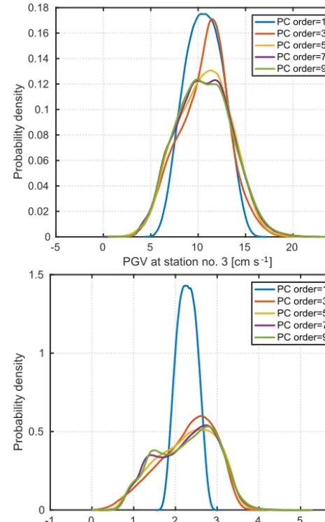
Apart from the above error estimates, the convergence of PC surrogate models with respect to truncation order is also investigated from a statistical point of view. Figure 4 shows PGV distributions from PC resampling on a 1 million mem-ber LHS set (P_LHS1E6) at two selected stations, with increasing odd PC truncation orders up to degree 9. It is seen that when the truncation order is larger than 5, the difference in the PGV prediction distributions becomes relatively small, suggesting that our ninth-order PC expansions are sufficiently accurate for the source model under consideration.

We finally compare distributions of PC and source model predictions; see Fig. 5. It is observed that our PC surrogate models are capable of reproducing PGV distributions pro-duced from source model realizations of the validation set P_LHSvalid. Besides, the excellent agreement between the two PC-predicted distribution curves in Fig. 5 suggests that our ex-isting 8000-model-simulation ensemble is statistically rep-resentative, which provides additional confidence in our PC representations.

3.2 PC statistics

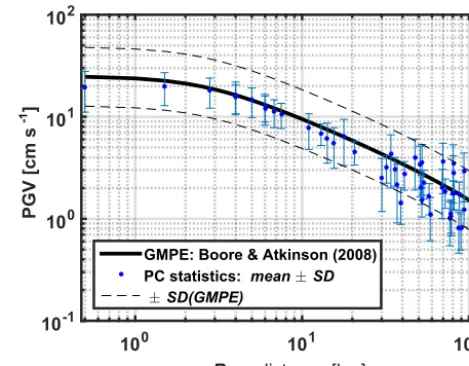
The PC surrogate models obtained in the previous section provide immediate access to prediction statistics, as given by Eqs. (5) and (6). Figure 6 shows means and standard devia-tions of PC PGV predicdevia-tions at different stadevia-tions, along with a reference median PGV curve predicted by the GMPE in Boore and Atkinson (2008)4_{. It is noted that two stations with}

4_{The interested reader is referred to Mai (2009),}

http://www.opensha.org/glossary-attenuationRelation-BOORE_

ATKIN_2008 (last access: 20 December 2017) and

http://www.gmpe.org.uk/gmpereport2014.pdf (last access: 20 December 2017) for more details on the GMPE employed in this paper.

-5 0 5 10 15 20 25

PGV at station no. 3 [cm s ] 0

0.02 0.04 0.06 0.08 0.1 0.12 0.14 0.16 0.18

Probability density

PC order=1 PC order=3 PC order=5 PC order=7 PC order=9

-1 0 1 2 3 4 5 6

0.5 1 1.5

Probability density

PC order=1 PC order=3 PC order=5 PC order=7 PC order=9

1

-1

Figure 4.PC-predicted PGV distributions at two selected stations (as indicated in Fig. 2). Distribution curves are obtained using ker-nel density estimation (Sheather and Jones, 1991) from PC realiza-tions on a 1 million member LHS setP_LHS1E6.

(6)

(quanti-0 5 10 15 20 25 30 PGV at station no. 3 [cm s ]

0 0.02 0.04 0.06 0.08 0.1 0.12 0.14

Probability density

0 1 2 3 4 5 6

0.1 0.2 0.3 0.4 0.5 0.6

Probability density

1

-1

Figure 5.Comparison of PGV distributions predicted by the source model (blue solid curve) and PC surrogate model (red dashed curve), respectively, at selected stations (as indicated in Fig. 2) over the validation sample setP_LHSvalid. The black dash-dotted curves are PGV prediction distributions obtained from PC surrogate model realizations on a 1 million member LHS setP_LHS1E6. Distributions are obtained using kernel density estimations (Sheather and Jones, 1991).

fied by the standard deviation bars) seems to decrease with increasingR_JBdistance as well.

The conditional mapping from canonical PC random vari-ables (ξ) to physical fault plane configurations makes it

diffi-cult to isolate the relative impact of individual parameters. To address this difficulty, we rely on the global sensitivity analy-sis (Homma and Saltelli, 1996; Sobol, 1993) and discuss the statistical significance of each canonical random parameters in the rupture model.

Figure 7 shows both the first- and total-order sensitivity indices associated with each random parameter at different stations. These sensitivity indices reveal that the model PGV response is most sensitive to the location of the hypocenter (xh is dominant andz_h plays a secondary role) throughout

R_JB distance [km]

100 101 102

PGV [cm s ]

10-1

100

101

102

GMPE: Boore & Atkinson (2008)

PC statistics: mean ' SD

' SD(GMPE)

-1

Figure 6. Comparison of PC statistics (based on uniform distri-bution assumption of the canonical PC random parameters) with GMPE results. Solid black curve denotes the median GMPE predic-tion, while the dashed lines are GMPE standard deviation bounds. Note that log scales are used in the plot.

10-5 10-4 10-3 10-2 10-1 100

1st-order sensitivities

J B 10-3

10-2

10-1 100

Total-order sensitivities

1

(a)

(b)

Figure 7.First-(a)and total-order(b)sensitivity indices at each station.

(7)

0 0.2 0.4 0.6 0.8 1

First-order sensitivities

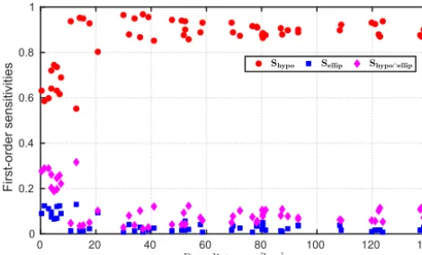
Figure 8.First-order sensitivity indices with respect to grouped pa-rameters.

stations (with R_JBdistance roughly more than 10 km away from the center), it is evident that at near-the-center stations, those elliptical patch parameters can still lead to a consider-able impact on PGV response.

To better illustrate the above sensitivity observation, we di-vided the parameters into the following two groups (ξ_hypo=

{ξ₂xh, ξ₃zh}andξ_ellip= {ξ₁AR, ξ₄a, ξ₅θ, ξ₆xc, ξ₇zc}; the superscripts denote the corresponding physical parameters) and calcu-lated the first-order sensitivity indices associated withξ_hypo

and ξ_ellip using Eq. (8a), denoted as _Shypo and _Sellip,

re-spectively. Note that the combined effect (interaction) of hypocenter location and elliptical patch parameters is simply given byShypo×ellip=1−Shypo−Sellip. The resulting group sensitivity indices are shown in Fig. 8. It is now clear that the hypocenter location alone is responsible for 80–90 % of the variability in PGVs at distant stations. Meanwhile, near the center, the hypocenter location alone is associated with only 55–75 % of the PGV variability, suggesting that the elliptical patch parameters play important roles with about 25–45 % contribution to the total PGV variability.

4 Bayesian inference

In this section, we utilize a Bayesian approach (Bernardo and Smith, 2001; Berger, 2013; Gelman et al., 2014) to find the most likely fault plane configuration, in the sense that the resulting earthquake rupture model produces PGVs that best match the reference GMPE curve for the same mag-nitude and focal mechanism (Boore and Atkinson, 2008). To this end, we first obtain the GMPE-predicted PGVs at the stations shown in Fig. 2, denoted as d, which serve

as observational data in our Bayesian inference, and com-pare d with our PC surrogate model predictions ed(ξ)= (Qe1(ξ),Qe2(ξ), . . .,QeNobs(ξ))T.

4.1 Bayesian formulation

To formulate the Bayesian problem, we start with Bayes’ for-mula:

p(η_|d)=p(d|η)p(η)

p(d) ∝p(d|η)p(η), (10) whereη is the parameter vector to be inferred,p(η)is the prior probability distribution ofη, and p(d|η)is the likeli-hood of observingd givenη. The denominatorp(d)is the marginal distribution known as evidence. (Note that this ev-idence can be neglected, as the MCMC sampling method (Haario et al., 2001; Roberts and Rosenthal, 2009) utilized below solely relies on the proportionality.) We adopt the as-sumption of independent Gaussian error at each station lo-cation; i.e., the discrepancy between observations (GMPE-predicted PGVs) and PC predictions at each station is an in-dependent Gaussian variable:

p(j)=p(dj−edj)= 1

√

2π σ2exp "

−(dj−edj)2 2σ2

#

, (11)

∀j∈ {1,2, . . ., N_obs}.

Recall that the PC prediction variability seems to decrease withR_JB distance according to Fig. 6. To account for this decay of PGV variance with R_JB distance in the Bayesian inference analysis, we partition theN_obs stations into four groups according to their correspondingR_JBdistances as in-dicated in Fig. 2, and associate each group of stations with a hyperparameterσ_{l(j )}2 (l(j )∈ {1,2,3,4}depending on the R_JB distance of thejth station). As a result, the likelihood can be expressed as

p(d|η)= Nobs

Y j₌1

1 q

2π σ2 l(j )

exp −(dj−edj(ξ))2 2σ_{l(j )}2

!

, (12)

and accordingly the inference parameter vectorηreads η=(ξ₁, ξ₂, . . ., ξ₇, σ₁2, σ₂2, . . ., σ₄2)T. (13) Our numerical experiments suggest that the 4−σ2 model above outperforms the model with only one hyperparameter for all stations. It is noted that we limit the number of uncer-tainty hyperparameters (σ2

i values) to four in this study, due to the limited number of observations (PGVs at limited num-ber of stations). If more observations were available, it might be beneficial to increase the number of hyperparameters.

The prior distribution ofη, without additional information

on the model parameters, is usually given by assumptions of uniform distribution for canonical PC parametersξ, and

Jef-frey’s priors (Sivia and Skilling, 2006) for hyperparameters σ_l2(asσ_l2is always greater than zero); consequently,

p(η)=   

1 2

7 4 Q l₌1

1

σ_l2 ∀ξ∈4 and ∀σ 2 l >0,

0 otherwise,

(8)

and Bayes’ rule reduces to

p(η|d)∝p(d|η)p(η)= (15)

              

Nobs

Q j=1

1 q

2π σ_{l(j )}2

exp −(dj−edj(ξ))2 2σ2

l(j ) !

∀ξ∈4and

" 1

2 7 4

Q l=1

1 σ_l2

#

∀σ_l2>0,

0 otherwise.

We rely on the adaptive metropolis MCMC approach (Haario et al., 2001; Roberts and Rosenthal, 2009) to sam-ple the above posterior distribution. It is worth noting that MCMC methods, despite the improved efficiency against tra-ditional MC approaches, generally require a large number of samples (typically tens of thousands, and even larger depend-ing on the dimensionality of the problem). This is one of the main reasons why we utilize PC techniques, as the use of the corresponding PC surrogates in the MCMC simulation leads to significant reduction in computational cost. In this study, the MCMC sample size for inference is set to 106.

4.2 Inference results

As mentioned above, we exploit the PC surrogate models in Bayesian inference analysis and update the posterior distri-bution of random parameters (ξ∈4), as well as PGV

pre-diction uncertainties (σ2

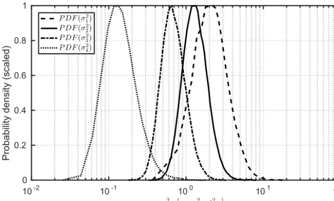
l values), in light of the GMPE ob-servations. Figure 9 shows the posterior probability distribu-tions of hyperparametersσ_l2(l∈ {1,2,3,4}). It is evident that σ_l2decreases withRJBdistance (froml=1 tol=4), which supports our previous ansatz from Fig. 6.

Similarly, we examine the sampling chains of PC ran-dom parametersξi(i∈ {1,2, . . .,7}). While some parameters (e.g.,ξ₁, ξ₂, ξ₃, andξ₆) yield very informative posterior dis-tributions (not shown here), others look relatively less infor-mative. It is noted that our goal is to estimate the posterior distributions of the physical parameters in Table 2, instead of the PC parameters. Thus, it is desired to map theξ chain

into the corresponding physical configuration chain, before inferring the most likely fault plane configuration.

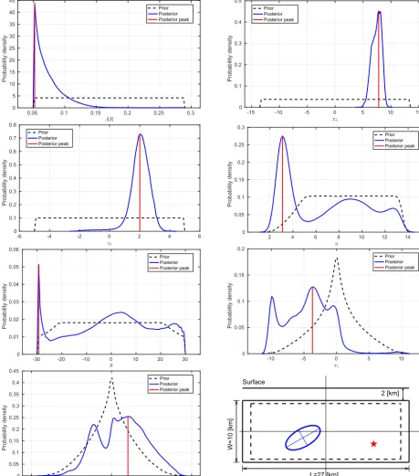
Figure 10 shows the posterior distributions of the physi-cal parameters after mapping from the PC parameter chain ofξ, as well as the corresponding inference of the fault plane

configuration (bottom right panel). It is observed that in light of the GMPE PGV observations (1) the hypocenter location (x_h and z_h) is well identified; (2) the size of the elliptical patch seems to be more likely near the lower bound of the prior; (3) the inclination angle of the elliptical patch, as well as the location of the patch, are less conclusive. For exam-ple, despite the clear peak in the inclination angle plot, the posterior distribution is relatively flat, suggesting limited in-formation gain compared with the prior knowledge. Further-more, thex_cdistribution only shows the fact that the ellipse tends to be in the left half of the fault plane; the definite

lo-cation of the elliptical patch (eitherxcor zc) is ambiguous. These findings are generally consistent with the results of the sensitivity analysis. Since the model is primarily sensitive to the hypocenter location, perturbing the hypocenter location leads to more effective adjustment in PGV responses. On the other hand, elliptical patch parameters have relatively small impact on PGV variance, which calls for more observational data to pin down those parameters.

One needs to be cautious about the Bayesian inference re-sults discussed above. From the physical point of view, the spatial distribution of those stations (see Fig. 2) where PGVs are reported is almost “symmetric” about the center of the fault plane (x=0 andy=0); as a result, one would expect to see a “symmetric” twin configuration that is roughly equally plausible from the Bayesian inference. However, this “sym-metric” counterpart is clearly missing in the above inference results. This is probably because when MCMC chain con-verges to the high probability region of hypocenter location in the bottom right quadrant of the fault plane, it becomes more and more difficult to escape from this high probability region and explore the other side of parameter space. In other words, there could be bimodal structures in the distributions ofx_h(as well asx_c) which the previous MCMC process fails to identify (e.g., the configuration in which the hypocenter is located in the bottom left quadrant of the fault plane, and the ellipse is centered at somewhere on the right half of the fault plane). While in theory it is possible to identify the missing multimodal distributions of random parameters by further in-creasing the number of MCMC samples, the computational cost can be excessive. Alternatively, we verify our expecta-tion of seeing the “symmetric” counterpart configuraexpecta-tion by rerunning the MCMC simulation starting with the “symmet-ric” counterpart configuration (i.e., with hypocenter being in the bottom left quadrant of the fault plane, and elliptical patch being on the right side of the fault plane). The result-ing fault plane configuration inference is shown in Fig. 11. As expected, the new MCMC process ended up with a fault plane configuration that is roughly “symmetric” to the previ-ous inference result, especially for the hypocenter location. The asymmetric behavior of the elliptical patch stems from the fact that (1) theN_obs stations are not exactly symmetri-cally distributed; thus, one should not expect exact symme-try; (2) as discussed before, the PGV responses are less sen-sitive to the elliptical patch properties, leading to ambiguity in inferring these properties.

4.3 Inference with restricted prior

(9)

10-2 10-1 100 101 102 0

0.2 0.4 0.6 0.8 1

Probability density (scaled)

Figure 9.Posterior probability distributions of prediction uncertainty parameters (each PDF curve is scaled to have unit peak height for better comparison).

In this section, we consider the following restrictions in our inference analysis:

R-1. The elliptical patch is inside the dashed rectangle

[L0, W0] =0.9× [L, W]shown in Fig. 1.

R-2. The area ratio of the elliptical patch (AR) is between 15 and 29 % of the fault plane area, i.e., 0.15<AR<0.29. R-3. The elliptical patch is not too elongated, i.e., the axis

ratio a b ≤3.

R-4. The hypocenter is located outside but near the ellip-tical patch, i.e., x_h=(a+3ζ_h₁)cos(2π ζ_h₂) and z_h= (b+b3_aζ_h₁)sin(2π ζ_h₂)∀(ζ_h₁, ζ_h₂)∈ [0,1]2.

One of the advantages of having previous PC surrogate models (which were built based on uninformative prior that spans a wide range of feasible scenarios, i.e., minimal re-strictions as in Table 2) is that the above four additional pa-rameter restrictions can be efficiently performed a posteriori, namely without the need for performing new model simula-tions (Alexanderian et al., 2012).

To begin with, we first incorporate the above restrictions into the Bayesian framework, namely by modifying the pre-vious prior distribution (Eq. 14) as follows:

p∗(η)=           

1 2

7 4 Q l₌1

1

σ_l2 ∀ξ∈4,∀σ 2 l >0 and all restrictions are satisfied,

0 otherwise.

(16)

However, due to the strong restrictions listed above, the support of the above prior probability distribution (Eq. 16)

turns out to be extremely limited in the parameter space

4, leading to computationally inefficient MCMC sampling

(since most of the samples drawn from a proposal distribu-tion will end up not satisfying at least one of the restricdistribu-tions and thus zero prior probability). To mitigate the difficulty of inefficient sampling due to restricted prior distribution, we introduce a new layer of parameterization, mapping from

4to restricted physical configurations. (Details on this new

mapping mechanism are given in Appendix B.)

Figure 12 shows the MCMC process of drawing random samples from proposal distributions and calculates the re-sulting posterior probability. Without additional restrictions (orange path), the parameter vectorζ=ξ, and the whole

pro-cess reduces to the standard MCMC propro-cess we used in the previous section. By introducing the new parameterization process (see Algorithm 2), we are transforming the original problem, which is based on PC parameter vectorξ, into a

new inference problem based onζ(we denoteζas the

auxil-iary random parameter vector hereafter, to distinguish it from the PC parameter vectorξ). This transformation is based on

the mapping fromζtoξ(i.e.,ξ₌ξ(ζ)) via their commonly

associated physical configuration. For clarity, we formulate the newζbased Bayesian problem as follows:

p(η∗|d)∝ (17)

                

" 1

2 7 4

Q l=1

1 σ_l2

# Nobs

Q j=1

1 q

2π σ2 l(j )

exp −(dj−edj(ξ(ζ)))2 2σ_{l(j )}2

!

∀ζ∈4,∀σ_l2>0,

0 otherwise.

(10)

0.05 0.1 0.15 0.2 0.25 0.3 AR

0 5 10 15 20 25 30 35 40 45

Probability density

Prior Posterior Posterior peak

-15 -10 -5 0 5 10 15

xh

0 0.1 0.2 0.3 0.4 0.5

Probability density

-6 -4 -2 0 2 4 6

zh

0 0.1 0.2 0.3 0.4 0.5 0.6 0.7 0.8

Probability density

2 4 6 8 10 12 14

a

0 0.05 0.1 0.15 0.2 0.25 0.3

Probability density

-30 -20 -10 0 10 20 30

θ

0 0.01 0.02 0.03 0.04 0.05 0.06

Probability density

-10 -5 0 5 10

xc

0 0.05 0.1 0.15 0.2

Probability density

-5 0 5

zc

0 0.05 0.1 0.15 0.2 0.25 0.3 0.35 0.4 0.45

Probability density

2 [km]

X

Z Surface

L=27 [km]

W=10 [km]

1

Figure 10.Prior (dashed black, derived from uniformξdistribution in4) and posterior (solid blue) distributions of physical fault plane configuration parameters. The bottom right panel shows the inferred fault plane configuration.

Following the same analysis as discussed before, we show the inference results under restrictions in Fig. 13. Note that the prior distributions of those physical parameters are differ-ent from those in Fig. 10, as the new ones are derived from uniformly distributed auxiliary random vectorζ∈4, instead

of PC parameters ξ∈4. Nevertheless, we see very

(11)

2 [km]

X

Z Surface

L=27 [km]

W=10 [km]

Figure 11. Inferred fault plane configuration with MCMC chain starting from the “symmetric” counterpart configuration.

differences are directly stemming from restrictions R-2 and R-3.

Though it is not obvious to see from Fig. 13, the re-stricted Bayesian MCMC process is indeed aware of the ex-istence of the “symmetric” counterpart configuration. Fig-ure 14 shows the restricted Bayesian MCMC sample chains of both the hypocenter (Fig. 14a) and elliptical patch center (Fig. 14b). It is seen that despite the fact the hypocenter sam-ples are mostly clustered around x_h=5 km, there is a sam-ple cloud on the opposite side (xh= −5 km), corresponding to the “symmetric” counterpart configuration discussed be-fore. The sample cloud of the elliptical center also shows bi-modal distributions, with primary cloud on the left (xc<0) and secondary “symmetric” counterpart on the right (around x_c=5 km). The correspondence betweenx_handx_cis shown in Fig. 14c, from which it is seen that whenx_his positive, x_c is more likely to be negative, and vice versa, suggesting that hypocenter and ellipse center are on the opposite side of the fault plane, as previous inference results suggested. Note that in this restricted Bayesian MCMC sampling, the total number of samples remains 106. The ability to observe the “symmetric” counterpart clouds is probably due to the fact that by introducing the auxiliary parameter ζ, we

dramati-cally shrunk the sampling space (it is only a small subspace of the original unrestricted parameter space). As mentioned before, introducing the auxiliary parameterζleads to

signif-icant efficiency improvement in the MCMC sampling pro-cess.

4.4 Comparing PGVs

We summarize the Bayesian analysis by comparing PC-predicted PGV responses to the three inferred fault plane configurations discussed above with the reference GMPE curve (see Fig. 15 and Table 3). We observe that all three configurations lead to a relatively close match between PC predictions and the reference GMPE curve. By comparing either the root mean square (rms) error or the relative rms error (see Table 3), we conclude that the red dots (corre-sponding to the unrestricted inference in Fig. 11) clearly

show larger discrepancy from the GMPE curve, suggesting smaller likelihood compared to the other two, consistent with our Bayesian analysis. When comparing the blue and green dots (unrestricted inference in Fig. 10 versus restricted infer-ence in Fig. 13), the former seems to be slightly better, which is expected because of the additional flexibility in fitting the GMPE curve. Nevertheless, it might be better to report the re-stricted inference results (configuration in Fig. 13), as it satis-fies all the restrictions learned from previous studies while re-taining plausible agreement with the reference GMPE curve.

5 Conclusions

An earthquake rupture model was adopted to explore the stochastic dependence of ground motion (in terms of PGVs) on random fault plane configurations. Thanks to the ability to generate two independent source model simulation ensem-bles with 8000 members each, we were able to build suc-cessful PC surrogate models to assess PGV responses over the virtual network ofN_obs=56 stations from one ensemble, and then to validate the quality of PC models on the other. Our statistical analysis showed that the two 8000-member LHS ensembles of source model simulations are adequate to represent the underlying PGV distributions at all stations, as they closely match with PC-predicted distributions over a much larger sample set.

A global sensitivity analysis of PC surrogate models was conducted. The analysis revealed that the source model PGV response is primarily sensitive to the hypocenter location, and much less sensitive to properties of the asperity patch, especially at stations far away from the fault plane (in terms of theR_JBdistance). While this holds true for all stations, it is noted that asperity patch properties still carry considerable impact (20–30 % associated variability) on PGV responses at stations close to the fault plane, and even more influence (ad-ditional 10 % variability) if one takes into consideration the interaction between asperity patch and hypocenter location.

Our analysis of PGV variabilities indicated that one needs to be cautious when interpreting PGVs at near-fault-plane stations, as they are more prone to higher model noise. This is supported by the Bayesian inference analysis, in which four independent model noise parameters (σ2

l for l=1,2,3,4) were introduced and assigned to four groups of observational stations, depending on their RJB distances away from the fault plane. The Bayesian inference results clearly showed the decreasing trend of noise parameters (σ_l2 values) when moving away from the fault plane (see Fig. 9). Further re-finement of the noise parameter profile along the R_JB dis-tance, though desired, is prohibited by the limited number of available observational stations.

(12)

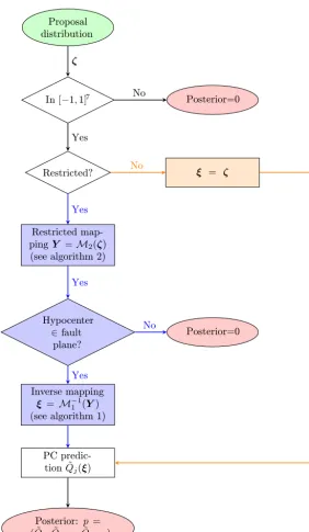
Figure 12.Flow chart demonstrating the random sampling process and the calculation of posterior probability in MCMC. The orange path corresponds to unrestricted sampling process, whereas the blue path incorporates additional restrictions on fault plane configurations. Note thatYdenotes the fault plane configuration vector in the physical domain, e.g.,Y₌(AR, x_h, z_h, a, θ, x_c, z_c)T.

have the hypocenter located in the lower right quadrant of the fault plane, and the elliptical patch centered in the lower left quadrant. (2) Due to the considerable “symmetry” presented by thoseN_obsstations, the most profound fault plane config-uration, which best reproduce the reference GMPE predic-tions, can potentially have a “symmetric” twin configuration, especially for the hypocenter location. (3) The restricted in-ference results remain consistent with the unrestricted ones, with slightly more deviation from the chosen GMPE

(13)

0.14 0.16 0.18 0.2 0.22 0.24 AR

0 5 10 15

Probability density

-15 -10 -5 0 5 10 15

xh

0 0.1 0.2 0.3 0.4 0.5

Probability density

-6 -4 -2 0 2 4 6

zh

0 0.1 0.2 0.3 0.4 0.5 0.6 0.7 0.8

Probability density

3 4 5 6 7 8

a

0 0.1 0.2 0.3 0.4 0.5 0.6 0.7

Probability density

-30 -20 -10 0 10 20 30

θ

0 0.01 0.02 0.03 0.04 0.05 0.06

Probability density

-10 -5 0 5 10

xc

0 0.05 0.1 0.15 0.2 0.25 0.3 0.35 0.4 0.45

Probability density

-3 -2 -1 0 1 2

zc

0 0.1 0.2 0.3 0.4 0.5 0.6

Probability density

2 [km]

X

Z Surface

L=27 [km]

W=10 [km]

1

Figure 13.Prior (dashed black, derived from uniformζ distribution in4) and posterior (solid blue) distributions of physical fault plane

configuration parameters in restricted inference. The bottom right panel shows the inferred fault plane configuration.

The analyses and findings in this study provide useful in-sights on how near-source ground shaking (and its variabil-ity) depends on random fault rupture configurations. Inter-estingly, even very simple source models (with elliptical slip patches) are able to generate shaking distributions that well reproduce empirical predictions. To better reproduce the

(14)

pri-Table 3.Comparison of PC-predicted PGVs of different inferred configurations with the reference GMPE curve. Unrestricted-1 and -2 correspond to inferences in Figs. 10 and 11, respectively. Each inferred configuration leads to PGV predictions in Fig. 15, as indicated by different colors.

Inference =

r

PNobs

j=1(Qej−QGMPEj )2

Nobs r= s

1 Nobs

PNobs

j=1

e

Qj−QGMPEj

QGMPE_j

2

Unrestricted-1 (blue) 1.1135 0.3395

Unrestricted-2 (red) 1.7413 0.3993

Restricted (green) 1.4564 0.3702

Figure 14. Restricted Bayesian MCMC sample chains of the hypocenter(a)and elliptical patch center(b); panel(c)shows the correspondence betweenx_handxcchains.

marily limited by the number of available stations at which PGVs are reported. By increasing the number of PGV report-ing stations, one may improve the Bayesian inference results (e.g., removing the ambiguity in inferring the elliptical patch location).

R_JB distance [km]

100 101 102

P

G

V

[c

m

s

-1]

10-1 100 101 102

GMPE: Boore & Atkinson (2008) ' SD(GMPE)

PC: unrestricted inference PC: unrestricted inference (symmetric) PC: restricted inference

Figure 15.Comparison of PC-predicted PGV responses with afore-mentioned three inferred fault plane configurations with the refer-ence GMPE curve. Dashed lines are standard deviation bounds of GMPE predictions.

Code and data availability. The COMPSYN code (Spudich and

(15)

Appendix A: Mapping from PC random parameters to physical parameters

Algorithm 1Unrestricted mapping – PC random parameter

ξ to physical parameters:Y =M₁(ξ)

1: Input_∀ξ₌(ξ₁, ξ₂, . . . , ξ₇)T _∈4

2: AR=0.05+1₂(ξ₁+1)(0.29−0.05) {Mapξ₁to area ratio} 3: x_h= −L₂+1₂(ξ₂+1)L {Map(ξ₂, ξ₃)to hypocenter location

(x_h, z_h)}

4: z_h_{= −}W₂ ₊1₂(ξ₃₊1)W 5: a_min₌

q AR·L·W

π {Calculate the lower bound ofafrom AR above}

6: a=a_min+1₂(ξ₄+1)(L₂ −a_min) {Mapξ₄toa, and calculate b}

7: b=AR_{π a}·L·W

8: ifzr_max(a, b,30◦) >W₂ then 9: Solve Eq. (A7) forθ∗

10: letθˆ=θ∗ {Calculate maximum feasible rotation angleθˆ} 11: else

12: letθˆ₌30◦ {Prescribe maximum feasible rotation angle otherwise}

13: end if

14: θ= − ˆθ+ ˆθ (ξ₅+1) {Mapξ₅to rotationθ}

15: Plug(a, b, θ )into Eq. (A4) to calculatex_maxr andz_maxr

16: xc∈ [xmin_c , x_cmax] = [−L₂+x_maxr ,L₂−xr_max]

17: zc∈ [zmin_c , zmax_c ] = [−W₂ +zr_max,W₂ −zr_max]

18: xc=x_cmin+1₂(ξ₆+1)(x_cmax−xmin_c ) {Map(ξ₆, ξ₇)to ellipse center(x_c, z_c)}

19: z_c=zmin_c +1₂(ξ₇+1)(zmax_c −zmin_c )

20: returnY=(AR, x_h, z_h, a, θ, x_c, y_c)T {Return parameter vector in the physical domain}

Letaandbbe the lengths of semi-major and minor axes, respectively, of the elliptical patch considered in the fault plane configuration discussed in Sect. 2, and AR be the area ratio defined by AR=π ab

LW (here,L=27 km andW=10 km are the length and width of the fault plane). The elliptical patch centered at the origin (x_c=0 and z_c=0, note the z axis is pointing downwards as shown in Fig. 1), when not ro-tated (meaningθ=0, the semi-major axis align withxaxis), can be expressed as

x z

=

acosβ bsinβ

where −π≤β≤π. (A1)

If the elliptical patch is rotated by θ∈ [−30◦,+30◦] (a positive angle denotes clockwise rotation), then the ellipse is given by

xr zr

=

_cosθ

−sinθ sinθ cosθ

x z

(A2)

=

_cosθ

−sinθ sinθ cosθ

acosβ bsinβ

=

acosθcosβ−bsinθsinβ asinθcosβ+bcosθsinβ

.

To ensure the resulting elliptical patch is completely con-fined within the fault plane, we first find the maximum extent of the ellipse in bothxandydirections. We first calculate the following twoβ∗values:

∂xr

∂β = −acosθsinβ−bsinθcosβ=0

⇒β_x∗=tan−1

−b

atanθ

(A3) ∂zr

∂β = −asinθsinβ+bcosθcosβ=0

⇒β_z∗=tan−1 _b

a 1 tanθ

.

Next, by substituting the aboveβ_x∗andβ_z∗into Eq. (A2), we have

x_maxr = |acosθcosβ_x∗−bsinθsinβ_x∗| (A4) zr_max= |asinθcosβ_z∗+bcosθsinβ_z∗|.

These are the maximum extents of the ellipse inxandy di-rections, respectively.

When the ellipse is not centered at the origin (xc6=0 and/orz_c6=0), the following conditions need to be satisfied:

|x_c| +xr_max≤ L

2 (A5)

|z_c| +zr_max≤W 2 , which leads to

|x_c| ∈

0,L 2 −x

r max

(A6)

|z_c| ∈

0,W 2 −z

r max

.

Note that the above constraint onx_c is always valid, since x_maxr ≤a≤L₂, while the z_c constraint requires more treat-ment aszr_maxcan be greater than W₂ under some rotation an-gleθ and semi-major axis a. To ensure thatzr_max≤ W₂, we first check if the prescribed upper bound rotation (30◦_{) is}

fea-sible. If not, we solve the following equation forθ∗, which corresponds to the maximum feasible rotation angle givena and AR:

zr_max=asinθ∗cosβ_z∗(θ∗, a,AR) (A7)

+bcosθ∗sinβ_z∗(θ∗, a,AR)= W

2 , and define the upper bound of the rotation angle as

ˆ

(16)

The resulting rotation angle parameterθ is then assumed to be uniformly distributed over[− ˆθ,θˆ].

The mapping fromξ to physical parameters is outlined in

the Algorithm 1. With the prior assumption of uniform dis-tribution of ξ in4, the corresponding prior distributions of

each physical parameter are shown in Fig. 10 (dashed black curves).

Appendix B: Restricted mapping

We introduce the auxiliary parameter vectorζ_∈4and

de-sign the following mapping process to generate fault plane configuration samples that satisfy our prior configuration re-strictions. For clarity, we list again the four restrictions be-low:

R-1. The elliptical patch is inside the dashed rectangle ([L0, W0] =0.9× [L, W]) shown in Fig. 1.

R-2. The area of the elliptical patch (AR) is between 15 and 29 % of the fault plane area, i.e., 0.15<AR<0.29. R-3. The elliptical patch is not too elongated, i.e.,a

b<3. R-4. The hypocenter is located outside but near the

ellip-tical patch, i.e., x_h=(a+3ζ_h₁)cos(2π ζ_h₂) and z_h= (b+b3_aζ_h₁)sin(2π ζ_h₂)∀(ζ_h₁, ζ_h₂)∈ [0,1]2.

The mapping process is similar to the one in Algorithm 1, with necessary modifications to satisfy the above conditions. We outline the constrained mapping in Algorithm 2. Note that there is one additional condition needs to be verified, i.e., whether or not the hypocenter is inside the fault plane, as it is not guaranteed by the mapping process (this is also indicated in Fig. 12).

Algorithm 2Restricted mapping – auxiliary parameter vec-torζto physical parameters:Y=M₂(ζ)

1: Input∀ζ₌(ζ₁, ζ₂, . . . , ζ₇)T_∈4

2: [L0, W0] =0.9× [L, W] {Set the restricted rectangle dimension}

3: [AR∗

l,AR∗u] = [0₀..1581,0.29]

{Calculate area ratio range w.r.t

L0, W0_{, the upper bound (0.29)}

corresponds to the maximum circle in[L0, W0]

}

4: AR∗₌_AR_l₊1

2(ζ1+1) AR∗u−AR∗l _{Map

ζ₁to temporary area ratio AR∗_}

5: a_min=

q AR∗_·L0_·W0

π {Calculate the lower bound ofafrom

AR∗}

6: a=a_min+1₂(ζ₄+1)(L₂0−a_min) {Mapζ₄toa, and calculate b}

7: b₌AR∗_{π a}·L0·W0 8: AR=π ab

L·W {Calculate area ratio w.r.t the original rectangle

[L, W]}

9: x_h=a+3ζ2+₂1cos2πζ3+₂1 10: z_h=b+b_a3ζ2+₂1sin2πζ2+₂1

{Map(ζ₂, ζ₃)to hypocenter location(x_h, z_h), note the resulting (x_h, z_h)can be outside the fault plane, in which case the posterior probability is set to zero.

}

11: ifzr_max(a, b,30◦) >W₂0 then

12: Solve Eq. (A7) forθ∗(using AR∗) {Calculate maximum feasible rotation angleθˆ}

13: letθˆ₌θ∗ 14: else

15: letθˆ=30◦ {Prescribe maximum feasible rotation angle otherwise}

16: end if

17: θ= − ˆθ+ ˆθ (ζ₅+1) {Mapζ₅to rotationθ}

18: Plug(a, b, θ )into Eq. (A4) to calculatex_maxr andzr_max 19: xc∈hx_cmin, x_cmaxi=h−L₂0+x_maxr ,L₂0−xr_maxi 20: zc∈hzmin_c , zmax_c i=h−W₂0+zr_max,W₂0−zr_maxi

21: xc=x_cmin+1₂(ζ₆+1)xmax_c −xmin_c {Map(ξ₆, ξ₇)to ellipse center(xc, zc)}

22: z_c₌zmin_c ₊1₂(ζ₇₊1)zmax_c ₋zmin_c

(17)

Author contributions. In this study, HCJ and PMM created the

earthquake rupture model and generated both the training and vali-dation ensembles of model simulations for building PC surrogates. The PC-based statistical analysis and Bayesian inference were con-ducted by GL and OMK. IH provided invaluable insights and advice throughout this work.

Competing interests. The authors declare that they have no conflict

of interest.

Acknowledgements. Research reported in this publication was

supported in part by research funding from King Abdullah Univer-sity of Science and Technology (KAUST). The first author thanks KAUST for all the support during his postdoctoral fellowship. Earthquake rupture and ground-motion simulations have been carried out using the KAUST Supercomputing Laboratory (KSL) and we acknowledge the support of the KSL staff.

Edited by: Thomas Poulet

Reviewed by: two anonymous referees

References

Abrahamson, N. A., Silva, W. J., and Kamai, R.: Summary of the ASK14 ground motion relation for active crustal regions, Earthq. Spectra, 30, 1025–1055, 2014.

Alexanderian, A., Winokur, J., Sraj, I., Srinivasan, A., Iskandarani, M., Thacker, W. C., and Knio, O. M.: Global sensitivity analysis in an ocean general circulation model: a sparse spectral projec-tion approach, Comput. Geosci., 16, 757–778, 2012.

Arroyo, D. and Ordaz, M.: Multivariate Bayesian regression analy-sis applied to ground-motion prediction equations, part 1: theory and synthetic example, B. Seismol. Soc. Am., 100, 1551–1567, 2010a.

Arroyo, D. and Ordaz, M.: Multivariate Bayesian regression anal-ysis applied to ground-motion prediction equations, Part 2: Nu-merical example with actual data, B. Seismol. Soc. Am., 100, 1568–1577, 2010b.

Atkinson, G. M. and Boore, D. M.: Modifications to existing ground-motion prediction equations in light of new data, B. Seis-mol. Soc. Am., 101, 1121–1135, 2011.

Atkinson, G. M. and Silva, W.: Stochastic modeling of California ground motions, B. Seismol. Soc. Am., 90, 255–274, 2000. Berger, J. O.: Statistical decision theory and Bayesian analysis,

Springer Science & Business Media, 2013.

Bernardo, J. M. and Smith, A. F. M.: Bayesian Theory, Meas. Sci. Technol., 12, 221, https://doi.org/10.1088/0957-0233/12/2/702, 2001.

Boore, D. M. and Atkinson, G. M.: Ground-Motion Pre-diction Equations for the Average Horizontal Component of PGA, PGV, and 5 %-Damped PSA at Spectral Peri-ods between 0.01 s and 10.0 s, Earthq. Spectra, 24, 99–138, https://doi.org/10.1193/1.2830434, 2008.

Boore, D. M., Joyner, W. B., and Fumal, T. E.: Equations for es-timating horizontal response spectra and peak acceleration from

western North American earthquakes: a summary of recent work, Seismol. Res. Lett., 68, 128–153, 1997.

Chiou, B., Darragh, R., Gregor, N., and Silva, W.: NGA project strong-motion database, Earthq. Spectra, 24, 23–44, 2008. Cruz-Jiménez, H., Chávez-García, F. J., and Furumura, T.:

Differ-ences in attenuation of ground motion perpendicular to the mex-ican subduction zone between Colima and Guerrero: An expla-nation based on numerical modeling, B. Seismol. Soc. Am., 99, 400–406, 2009.

Debusschere, B., Sargsyan, K., Safta, C., and Chowdhary, K.: Un-certainty quantification toolkit (UQTk), Handbook of Uncer-tainty Quantification, 1–21, 2016.

Debusschere, B. J., Najm, H. N., Pébay, P. P., Knio, O. M., Ghanem, R. G., and Le Maıtre, O. P.: Numerical challenges in the use of polynomial chaos representations for stochastic processes, SIAM J. Sci. Comput., 26, 698–719, 2004.

Furumura, T. and Singh, S.: Regional wave propagation from Mex-ican subduction zone earthquakes: The attenuation functions for interplate and inslab events, B. Seismol. Soc. Am., 92, 2110– 2125, 2002.

Gelman, A., Carlin, J. B., Stern, H. S., and Rubin, D. B.: Bayesian data analysis, vol. 2, Chapman & Hall/CRC Boca Raton, FL, USA, 2014.

Ghanem, R. G. and Spanos, P. D.: Stochastic finite elements: a spec-tral approach, Springer-Verlag New York, 1991.

Giraldi, L., Le Maître, O. P., Mandli, K. T., Dawson, C. N., Hoteit, I., and Knio, O. M.: Bayesian inference of earthquake parame-ters from buoy data using a polynomial chaos-based surrogate, Comput. Geosci., 21, 683–699, 2017.

Haario, H., Saksman, E., and Tamminen, J.: An adaptive Metropolis algorithm, Bernoulli, 223–242, 2001.

Homma, T. and Saltelli, A.: Importance measures in global sensi-tivity analysis of nonlinear models, Reliab. Eng. Syst. Safe., 52, 1–17, 1996.

Irikura, K. and Miyake, H.: Recipe for predicting strong ground motion from crustal earthquake scenarios, Pure Appl. Geophys., 168, 85–104, 2011.

Le Maître, O. P. and Knio, O. M.: Spectral methods for uncertainty quantification: with applications to computational fluid dynam-ics, Springer Science & Business Media, 2010.

Mahani, A. B. and Atkinson, G. M.: Evaluation of functional forms for the attenuation of small-to-moderate-earthquake response spectral amplitudes in North America, B. Seismol. Soc. Am., 102, 2714–2726, 2012.

Mai, P. M.: Ground motion: Complexity and scaling in the near field of earthquake ruptures, in: Encyclopedia of Complexity and Sys-tems Science, Springer, 4435–4474, 2009.

Mai, P. M. and Beroza, G. C.: Source scaling properties from finite-fault-rupture models, B. Seismol. Soc. Am., 90, 604–615, 2000. Mai, P. M., Spudich, P., and Boatwright, J.: Hypocenter locations in finite-source rupture models, B. Seismol. Soc. Am., 95, 965–980, 2005.

(18)

Maufroy, E., Chaljub, E., Hollender, F., Bard, P.-Y., Kristek, J., Moczo, P., De Martin, F., Theodoulidis, N., Manakou, M., Guyonnet-Benaize, C., Hollard, N., and Pitilakis, K.: 3D numer-ical simulation and ground motion prediction: Verification, val-idation and beyond–Lessons from the E2VP project, Soil Dyn. Earthq. Eng., 91, 53–71, 2016.

McKay, M. D., Beckman, R. J., and Conover, W. J.: Comparison of three methods for selecting values of input variables in the analy-sis of output from a computer code, Technometrics, 21, 239–245, 1979.

Minson, S., Simons, M., Beck, J., Ortega, F., Jiang, J., Owen, S., Moore, A., Inbal, A., and Sladen, A.: Bayesian inversion for fi-nite fault earthquake source models–II: the 2011 great Tohoku-oki, Japan earthquake, Geophys. J. Int., 198, 922–940, 2014. Olson, A. H., Orcutt, J. A., and Frazier, G. A.: The discrete

wavenumber/finite element method for synthetic seismograms, Geophy. J. Int., 77, 421–460, 1984.

Roberts, G. O. and Rosenthal, J. S.: Examples of adaptive MCMC, J. Comput. Graph. Stat., 18, 349–367, 2009.

Seber, G. A. and Lee, A. J.: Linear regression analysis, vol. 329, John Wiley & Sons, 2012.

Sheather, S. J. and Jones, M. C.: A reliable data-based bandwidth selection method for kernel density estimation, J. Roy. Stat. Soc. B Met., 53, 683–690, 1991.

Singh, S., Srinagesh, D., Srinivas, D., Arroyo, D., Pérez-Campos, X., Chadha, R., and Suresh, G.: Strong Ground Motion in the Indo-Gangetic Plains during the 2015 Gorkha, Nepal, Earth-quake Sequence and Its Prediction during Future EarthEarth-quakes, B. Seismol. Soc. Am., 107, 1293–1306, 2017.

Sivia, D. and Skilling, J.: Data analysis: a Bayesian tutorial, OUP Oxford, 2006.

Sobol, I.: Sensitivity estimates for nonlinear mathematical models, Math. Model. Comput. Exp., 1, 407–414, 1993.

Somerville, P. G., Smith, N. F., Graves, R. W., and Abrahamson, N. A.: Modification of empirical strong ground motion attenu-ation relattenu-ations to include the amplitude and durattenu-ation effects of rupture directivity, Seismol. Res. Lett., 68, 199–222, 1997.

Somerville, P., Irikura, K., Graves, R., Sawada, S., Wald, D., Abra-hamson, N., Iwasaki, Y., Kagawa, T., Smith, N., and Kowada, A.: Characterizing crustal earthquake slip models for the prediction of strong ground motion, Seismol. Res. Lett., 70, 59–80, 1999. Spudich, P. and Xu, L.: 85.14-Software for Calculating Earthquake

Ground Motions from Finite Faults in Vertically Varying Media, Int. Geophys., 81, 1633–1634, 2003.

Sraj, I., Mandli, K. T., Knio, O. M., Dawson, C. N., and Hoteit, I.: Quantifying Uncertainties in Fault Slip Distribution during the T¯ohoku Tsunami using Polynomial Chaos, Ocean Dynam., 67, 1535–1551, https://doi.org/10.1007/s10236-017-1105-9, 2016. Sudret, B. and Mai, C.: Computing seismic fragility curves using

polynomial chaos expansions, in: Proc. 11th Int. Conf. Struct. Safety and Reliability (ICOSSAR-2013), Elsevier, New York, USA, 16–20 June 2013.

Thingbaijam, K. K. S., Martin Mai, P., and Goda, K.: New Empiri-cal Earthquake Source-SEmpiri-caling Laws, B. Seismol. Soc. Am., 107, 2225–2246, 2017.

Tinti, E., Fukuyama, E., Piatanesi, A., and Cocco, M.: A kinematic source-time function compatible with earthquake dynamics, B. Seismol. Soc. Am., 95, 1211–1223, 2005.

Van Den Berg, E. and Friedlander, M.: SPGL1: A solver for large-scale sparse reconstruction, available at: https://www.cs.ubc.ca/ ~mpf/spgl1/ (last access: 20 December 2017), 2007.

Van Den Berg, E. and Friedlander, M. P.: Probing the Pareto frontier for basis pursuit solutions, SIAM J. Sci. Comput., 31, 890–912, 2008.

Vyas, J. C., Mai, P. M., and Galis, M.: Distance and azimuthal de-pendence of ground-motion variability for unilateral strike-slip ruptures, B. Seismol. Soc. Am., 106, 1584–1599, 2016. Wells, D. L. and Coppersmith, K. J.: New empirical relationships

among magnitude, rupture length, rupture width, rupture area, and surface displacement, B. Seismol. Soc. Am., 84, 974–1002, 1994.