R E S E A R C H
Open Access
Sequential algorithm for life threatening cardiac
pathologies detection based on mean signal
strength and EMD functions
Emran M Abu Anas
1, Soo Y Lee
2, Md K Hasan
1,2** Correspondence: khasan@eee. buet.ac.bd
1Department of Electrical and Electronic Engineering, Bangladesh University of Engineering and Technology, Dhaka-1000, Bangladesh
Abstract
Background:Ventricular tachycardia (VT) and ventricular fibrillation (VF) are the most serious cardiac arrhythmias that require quick and accurate detection to save lives. Automated external defibrillators (AEDs) have been developed to recognize these severe cardiac arrhythmias using complex algorithms inside it and determine if an electric shock should in fact be delivered to reset the cardiac rhythm and restore spontaneous circulation. Improving AED safety and efficacy by devising new algorithms which can more accurately distinguish shockable from non-shockable rhythms is a requirement of the present-day because of their uses in public places. Method:In this paper, we propose a sequential detection algorithm to separate these severe cardiac pathologies from other arrhythmias based on the mean absolute value of the signal, certain low-order intrinsic mode functions (IMFs) of the Empirical Mode Decomposition (EMD) analysis of the signal and a heart rate determination technique. First, we propose a direct waveform quantification based approach to separate VT plus VF from other arrhythmias. The quantification of the electrocardiographic waveforms is made by calculating the mean absolute value of the signal, called the mean signal strength. Then we use the IMFs, which have higher degree of similarity with the VF in comparison to VT, to separate VF from VTVF signals. At the last stage, a simple rate determination technique is used to calculate the heart rate of VT signals and the amplitude of the VF signals is measured to separate the coarse VF from VF. After these three stages of sequential detection procedure, we recognize the two components of shockable rhythms separately. Results:The efficacy of the proposed algorithm has been verified and compared with other existing algorithms, e.g., HILB [1], PSR [2], SPEC [3], TCI [4], Count [5], using the MIT-BIH Arrhythmia Database, Creighton University Ventricular Tachyarrhythmia Database and MIT-BIH Malignant Ventricular Arrhythmia Database. Four quality parameters (e.g., sensitivity, specificity, positive predictivity, and accuracy) were calculated to ascertain the quality of the proposed and other comparing algorithms. Comparative results have been presented on the identification of VTVF, VF and shockable rhythms (VF + VT above 180 bpm).
Conclusions:The results show significantly improved performance of the proposed EMD-based novel method as compared to other reported techniques in detecting the life threatening cardiac arrhythmias from a set of large databases.
Background
Ventricular Fibrillation (VF) and Ventricular Tachycardia (VT) are life-threatening car-diac arrhythmias generally observed in adults with coronary artery disease. In 1979, automatic external defibrillators (AEDs) were introduced to accurately analyze the car-diac rhythms and, if appropriate, advise/deliver a high-energy shock to those patients who suffer from coarse VF and VT of a rate above 180 bpm, combinedly known as the shockable rhythms [6]. Though a significant number of works have been published on this topic, the scope for development of more accurate and reliable techniques relaxing assumptions of certain previous works and incorporating features from diverse nature of the cardiographic signals is yet open. Based on separation capability, the algorithms available in the literature can be classified into categories such as, separating VF from VT [4,7,8], VF from normal sinus rhythm (NSR) [9], VF plus VT from nonVTVF [10], shockable rhythms from other ECG pathologies [5,11,12], VF from nonVF [1-4,13-24]. Comprehensively, the last two categories [25] are the most realistic for fruitful hospital management of cardiac abnormalities.
detects the nonVF signal from ECG arrhythmias. But in the detection of VF, this method shows poor accuracy due to the false detection of the VF signal with low peak frequency in the spectrum [26]. On the other hand, the Hilbert transform (HILB) [1] and phase space reconstruction (PSR) [2] algorithms employing phase space plot of the ECG signal demonstrate improved performance of VF detection. Because the phase space plot is based on the histogram of a signal, it does not consider the shape of this signal. Thus, to separate VT from VF when other arrhythmias are also present, these two methods are not very suitable.
In this paper, we propose a sequential detection algorithm based on the mean abso-lute strength and certain low-order intrinsic mode functions (IMFs) of the EMD analy-sis of the signal along with a simple rate determination technique. In our proposed algorithm, we not only separate VF but also VT from other arrhythmias. VT plus VF (VTVF) is separated from other arrhythmias in the first stage using an index called the mean absolute value (MAV). Then we decompose the VTVF signal into IMFs using the EMD technique to discriminate VF from VT. EMD was introduced in [27] for pro-cessing signals from nonlinear and non-stationary processes. Here, we apply the EMD technique to biomedical signals and particularly for ECG analysis. Next, a simple rate determination algorithm is utilized to classify VT according to the heart rate and to separate coarse VF from fine VF, amplitude of the VF signals are measured. Finally, this sequential ECG arrhythmias classification approach is interpreted as three different detection schemes, such as, VTVF from nonVTVF; VF from nonVF; shockable from non-shockable rhythms. While proposing an algorithm for detecting the shockable rhythms special care must be taken to make the specificity high. It will then ensure the false alarm generation probability of the AEDs low. But an algorithm with high specifi-city generally results in low sensitivity. To mitigate this contradictory requirement, detection of the shockable rhythms using a sequential algorithm is found to be more effective. At last, in the ‘Results’ Section, we compare our algorithm with different well-known algorithms available in the literature.
Methods
ECG signals
annoted as the noise signals. Since, in this work we have no interest in these noise sig-nals, we have omitted these noise episodes. Also, analysis of the distinct mode asystole signal is not presented here. Therefore, this type of ECG signal is not included into our complete dataset.
The complete dataset includes the following types of ECG signals.
1. Normal beat
2. Left bundle branch block beat (LBBB) 3. Right bundle branch block beat (RBBB) 4. Atrial premature beat (APC)
5. Aberrated atrial premature beat 6. Nodal (junctional) premature beat
7. Supraventricular premature or ectopic beat 8. Premature ventricular contraction (PVC) beat 9. Fusion of ventricular and normal beat 10. Atrial escape beat
11. Nodal (junctional) escape beat 12. Paced beat
13. Fusion of paced and normal beat 14. Unclassifiable beat
15. Blocked APC
16. Ventricular tachycardia 17. Ventricular fibrillation
To determine the discriminating threshold and verify its effectiveness, the complete dataset is divided into two subsets: training and test datasets. The training dataset is used to determine the thresh-old value. To check the efficacy of the threshold value determined from the training dataset, the test dataset is used. Both the datasets include all types of above mentioned rhythms. The training dataset includes:
1. (1805 - 7) × 23 × 2 = 82708 episodes from MITDB (file no. 100-109, 111-119, 121-124).
2. 2000 episodes of VF and 2000 episodes of VT from VFDB.
On the other hand, the test dataset includes:
1. (1805 - 7) × 25 × 2 = 89900 episodes from MITDB (file no. 200-203, 205, 207-210, 212-215, 217, 219-223, 228, 230-234).
2. 2000 episodes of VF and 2000 episodes of VT from VFDB.
Classification of the ECG signals according to the AHA recommendations
According to the AHA recommendations, all ECG abnormalities are classified into fol-lowing categories [6]:
1. Shockable rhythms
2. Non-shockable rhythms • ‘NSR’: normal sinus rhythm.
• ‘N’: other arrhythmia, including supraventricular tachycardia, sinus bradycar-dia, LBBB, RBBB, APC and PVC beats.
• ‘Asyst’: asystole; ECG signal with a peak-to-peak amplitude of < 100μV, last-ing more than 4 s.
3. Intermediate rhythms
• ‘VT-lo’: slow ventricular tachycardia with a rate of < 180 bpm. • ‘fine VF’: any VF signal with an amplitude in the range 100 - 200μV.
It is clear from this classification that VT is divided into two categories according to heart rate; ‘VT-hi’and ‘VT-lo’. This VT classification considers border heart rate as 180 bpm. It is, however, not strict. It may be in the range 150 - 180 bpm. AEDs only advise/deliver shock to shockable rhythms, and intermediate rhythms are treated in a different way called anti-tachycardia pacing.
Detection of VTVF from other arrhythmias
To detect the life threatening cardiac arrhythmias, VT and VF, from other arrhythmias, we propose to use a property that does not match with that of any nonVTVF signal. Typical ECG waveforms of NSR, VT and VF are given in Figure 1. Here, NSR is treated as the representative of nonVTVF signals. The three waveforms are plotted in the same scale. From this figure we see that the width of the QRS complex is different for different arrhythmias. For NSR, it is noticed that the QRS interval is normally 0.06 - 0.10 sec and in case of VT, the QRS complex is more wider (> 0.10 sec). In VF, no QRS complex is noticed. On the other hand, P waves are normal (upright and uniform) in the NSR wave-form and in case of VT and VF signal, no P waves are observed [31].
0 1 2 3 4 5 6 7 8
0 0.5
1 (a) NSR
time (sec)
amplitide
0 1 2 3 4 5 6 7 8
−1 0
1 (b) VT
time (sec)
amplitude
0 1 2 3 4 5 6 7 8
−1 0 1
(c) VF
time (sec)
amplitude
The distinguishable morphological characteristics of these three groups, namely nonVTVF, VT and VF can be quantified using a term called the absolute strength of a signal. The absolute strength or the mean of absolute value (MAV) of a signalx(n) of lengthNis defined as
MAV
N x n
n N
=
( )
= −
∑
10 1
(1)
Here, nstands for the number of samples within the chosen length. In case of NSR,
the main representative of the nonVTVF group, the duration of the QRS complex is small as compared to one ECG period as illustrated in Figure 1(a). It is also observed from this figure that the NSR signal level is low for most of the time in an ECG cycle. Therefore, the absolute signal level of the QRS complexes dominates in the summation
of MAVcalculation (eqn. (1)). A lowMAVis thus obtained for such episodes. In case
of VT, we see that the QRS complex is much wider than that of NSR, and the ECG
signal hardly goes through the baseline as is the case for VF. Therefore, the MAVof
VT and VF for a fixed duration window is comparatively larger than that for the NSR. Before calculating the total MAV of a ECG signal, first it is necessary to normalize the ECG signal because the ECG signals collected from the different databases have
different dynamic value. Another important thing to be noted is that, to use theMAV
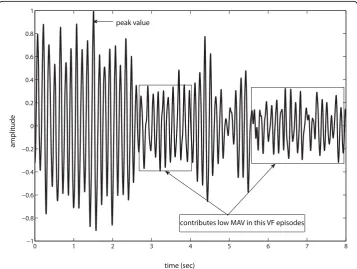
as the threshold parameter, we need to properly choose the analysis window duration. To understand the reason behind the necessity to appropriately choose the analysis
window duration, consider a normalized VF episode of 8-s length from cu01mfile of
CU database shown in Figure 2. If we choose an 8-s episode length, then it may
0 1 2 3 4 5 6 7 8
−1 −0.8 −0.6 −0.4 −0.2 0 0.2 0.4 0.6 0.8 1
time (sec)
contributes low MAV in this VF episodes peak value
amplitude
include a damped VF signal, as shown in figure 2, where most of the signal samples fall in the low amplitude range, and the MAV becomes low (e.g., 0.2577). Therefore, it is necessary to make the analysis window length small. Choosing an analysis window of too small duration (say, 1-s) creates the same problem as observed in the TCI
method. Here, we choose the 2-s window for analysis. After calculating the MAV of
this 2-s analysis window, we shift the analysis window by 1-s successively for other
seg-ments of 2-s within the 8-s ECG episode and calculate the MAVagain. After
comple-tion of shifting the analysis window to cover the whole decision frame, we average all
the MAVs found in each stage and finally MAV= 0.34 is found which is higher than
that obtained for the 8-s analysis window. In this way, by appropriately selecting the
analysis window length in calculating the MAV , we can overcome the effect of
damped behavior of the ECG signal.
Observation of other nonVTVF ECG waveforms such as Premature Ventricular Con-traction (PVC), Premature Atrial ConCon-traction (PAC), Supraventricular Tachycardia
(SVT) etc. reveals that these abnormalities also have low MAV compared to VT and
VF. For example, PVC arrhythmia has small MAV because a PVC beat contains only
wide QRS complex and no P waves or T waves are associated with this abnormal beat
[31]. Thus, we can use MAVas the performance index to discriminate the VTVF from
other arrhythmias.
In ECG analysis, it is important that we choose the episode length or decision frame appropriately. Decision frame should be taken in such a way that is neither too short to make a false alarm nor too long to cause severe cardiac arrest. Decreasing the epi-sode length from its optimum value results in a low accuracy but quick detection. On the contrary, increasing the episode length improves the accuracy up to a certain level but requires longer detection time.
The whole process of separating VT plus VF from other arrhythmias can be described as in the following:
1. Choose a segment of ECG signal of Le-second duration. This segmented ECG
signal ofLe-second duration should be stored for the second stage.
2. The segment of the ECG signal is preprocessed using the well-known filtering process as used in [32], which is carried out in a MATLAB routine, calledfiltering. m[33]. The filtering algorithm works in four successive steps.
•First, the mean value is subtracted from the signal.
•Second, a moving average filter is applied in order to remove the power line noise.
•Third, a drift suppression is carried out by a high pass filter with a cut-off fre-quency of 1 Hz.
• In the last step, a low pass Butterworth filter with a cut-off frequency of
30 Hz is applied in order to suppress the high frequency noise like intersper-sions and muscle noise.
All filters in the preprocessing step is implemented using the Matlab routine‘filtfilt’ function.
3. Then, choose a smaller segmentx(n) from the ECG signal ofLe-second duration
2Fs. For example, the sampling frequency of the ECG signal of the MITDB is 360
smaples/sec. Thus the length of the smaller segmentNis 2 × 360 = 720 samples.
4. Next, divide the smaller segmentx(n) by the maximum absolute value found in
that segment.
5. Calculate theMAVusing (1).
6. Shift the window by 1-s successively for other segments of 2-s within theLe
-sec-ond ECG episode and go through step (4) to (5).
7. Make decision on everyLe-second ECG episode (Le≥2) by averaging theLe- 1
consecutive values ofMAVobtained from theLe- 1 consecutive 2-s segments with
1-s step. The average value,MAVafor anLe-second episode is calculated as
MAV
Le MAV
a
i L
i e =
− =
−
∑
11
1 1
(2)
whereMAViis the value ofMAVin thei-th 2-s stage.
We calculate the MAVaof the three pathologies shown in Figure 1 and are obtained
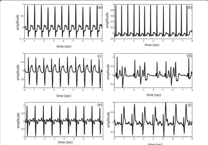
as 0.0765 (NSR), 0.3954 (VT) and 0.4116 (VF). To verify the effectiveness of the MAV index for separating the non-VTVF arrhythmias from the VTVF arrhythmias, other nonVTVF representatives namely, left bundle branch block beat, nodal (junctional)
premature beat (rate ≈100 bpm), high rate supraventricular tachycardia (rate≈ 100
bpm), premature ventricular contraction, right bundle branch block beat and paced beat are chosen from the ECG databases. These six pathologies are demonstrated in
Figure 3 and their MAVa are 0.1649, 0.0954, 0.1372, 0.1475, 0.1571, 0.2166,
Figure 3MAVof different ECG signals. ECG waveform and theMAVa values of different nonVTVF
pathologies. (a) Left bundle branch block beat,MAVa= 0.1649; (b) Nodal (junctional) premature beat,MAVa
= 0.0954; (c) High rate supraventricular tachycardia,MAVa= 0.1372; (d) Premature ventricular contraction,
respectively. Certainly, there is a clear separation of these MAVavalues with those
obtained from VT and VF episodes.
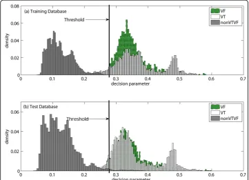
If MAVais greater than a certain thresholdMAVd, VTVF is detected. To determine
the thresh-old value, training dataset is used. Figure 4 shows the probability
distribu-tion of MAVa of the training dataset and the test dataset. The threshold value is
selected from the probability distributions of the training dataset shown in Figure 4(a) and we have chosenMAVd= 0.27 forLe= 8-s to ensure high specificity and also good
sensitivity. It is also noticed from Figure 4(b) that when we apply this threshold to the test dataset, high accuracy is still obtained.
Separation of VF from VTVF
Now that we have separated VTVF from other arrhythmias. In this stage, we separate VF from VT. Before we explain our motivation for using the EMD technique, we briefly describe what EMD is.
EMD Preliminaries
EMD is a signal decomposing method which is fully data-driven and does not require any a priori basis function [27,34]. The aim of the EMD is to decompose the signal into a sum of intrinsic mode functions (IMFs). An IMF is a function that satisfies two conditions: (1) in the whole data set, the number of extrema and the number of zero crossings must either be equal or differ at most by one; and (2) at any point, the mean value of the envelop defined by the local maxima and the envelop defined by the local minima is zero. An IMF represents the oscillatory mode embedded in the data as a counter-part to the simple harmonic function used in Fourier analysis [35].
Figure 4Probability histogram ofMAVa. Probability histogram of the decision parameterMAVa. (a)
Given a signal x(n), the starting point of the EMD is the identification of all the local maxima and minima. All the local maxima are then connected by a cubic spline [36] curve as the upper envelop eu(n). Similarly, all the local minima are connected by a
spline curve as the lower envelop el(n). The mean of the two envelops is denoted as
m1(n) = [eu(n)+el(n)]/2 and is subtracted from the signal. Thus the first componenth1
(n) is obtained as
x n( )−m n1( )=h n1( ) (3)
The above procedure to extract the IMF is called the siftingprocess. Ideally,h1(n)
should be an IMF, as the construction ofh1(n) seems to have been made to satisfy all
the requirements of IMF. Since h1(n) still contains multiple extrema in between zero
crossings, the sifting process is performed again onh1(n). This process is applied
repe-titively to the proto- IMF hk(n) until the first IMFc1(n), which satisfies the IMF
condi-tion, is obtained. Couple of stopping criteria are used to terminate the sifting process [27]. A commonly used criterion is the value of standard deviation, SD, computed from the two consecutive sifting:
SD= | ( )( ) ( )|
( )( )
h k n h k n
h k n
n N
1 1 1 2
12 1
0
− −
−
=
∑
(4)where, N is the total number of samples in x(n). When the SD is smaller than a
threshold, the first IMFc1(n) is obtained. Thenc1(n) is separated from the rest of the
data by
x n( )−c n1( )=r n1( ) (5)
It is to be noted that the residue r1(n) still contains some useful information. We can
therefore treat the residue as a new signal and apply the same sifting process to obtain
ri−1( )n −c ni( )=r ni( ), i= …1, ,q (6)
The whole procedure terminates when either the component cq(n) or the residuerq
(n) becomes very small or when the residue rq(n) becomes a monotonic function.
Combining (5) and (6) yields the EMD of the original signal,
x n c ni r n
i n
q
( )= ( ) ( )
=
∑
+1
(7)
The results of the decomposition are q –intrinsic modes and a residue. The lower
order IMFs capture the fast oscillation modes while the higher order IMFs typically represent the slow oscillation modes present in the underlying signal [27,37]. An exam-ple illustrating the Empirical Mode Decomposition is given in the‘Appendix’section.
QRS complex is absent in VF and as a result this pathology has more symmetric envel-opes than do other abnormalities and thus possesses narrowband characteristics. There-fore, to separate VF from VT, the EMD technique can effectively use the factors of
narrowband/wideband characteristics and symmetry/asymmetry property of a signal’s
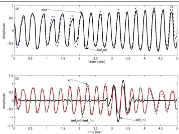
envelopes. Now, we apply the EMD technique on a VF episode to decompose it into IMFs and plot the original ECG signalx(n) along with its first IMF as shown in Figure 5 (a). From Figure 5(a) we can say that in case of VF, its first IMF is very much close to the original ECG signal. This is be-cause the VF has certain properties that well match the properties of the IMF as stated above. As the EMD technique cannot decompose an IMF signal further, therefore, in case of a VF episode, there is a unique relationship between the ECG signal and its first IMF. Here, unique relationship means that the ori-ginal ECG signal and its first IMF is very much similar. In some cases high frequency noise still remains in the ECG signal after preprocessing. Therefore, when we apply EMD to decompose the VF signal, the first IMF captures this high frequency noise as the fast oscillation mode illustrated in Figure 5(b). To overcome this effect we consider the sum of the first two IMFs instead of using only the first one. We can observe from Figure 5(b) that unique relationship still exists between the ECG signal and the sum of first two IMFs for the VF episode. In case of VT, this unique relationship or similarity between the ECG signal and the sum of its first two IMFs does not hold as illustrated in Figure 6 for both noise free and noise corrupted VT signals.
To exploit the property of unique relationship between the ECG signal and the sum of its first two IMFs that exists in case of the VF only, sum of the first two
IMFs from the ECG signal is subtracted and the MAV of the difference signal is
calculated. Since, the dynamic range of the ECG signal varies from database to
data-base, we normalize this MAVwith respect to the original ECG signal. In case of a
VF episode, the normalized MAV or NMAV of the difference signal is very small
than that of a VT episode. Here, we choose a 2-s analysis window as in the previous case. But in this case, the performance index (NMAV ) is less sensitive to the analy-sis window length.
The process of detecting VF from VTVF can then be described as below:
1. First, choose a segmentx(n) of duration 2-s andNsamples from the previously saved ECG signal ofLe-second duration.
2. At this stage, the ECG signal is preprocessed in three successive steps. •First, the mean value is subtracted from the signal.
•Second, a drift suppression is carried out by a high-pass filter with a cut-off frequency of 1 Hz.
•In the last step, a low-pass Butterworth filter with a cut-off frequency of 20 Hz and order 12 is applied to suppress the high frequency information.
3. Apply EMD onx(n) and determine
imf12( )n =imf n1( )+imf n2( )
where,imf1(n) andimf2(n) denotes the first and second IMFs, respectively.
4. Then, calculate the difference between the original signal and sum of its first two IMFs,
e n( )=x n( )−imf12( )n
0 0.5 1 1.5 2 2.5 3 3.5 4 4.5 5 −1
−0.5 0 0.5 1
time (sec)
Amplitude
(a)
0 0.5 1 1.5 2 2.5 3 3.5 4 4.5 5 −1
−0.5 0 0.5 1
time (sec)
Amplitude
(b)
imf1(n)+imf2(n)
imf
1(n)+imf2(n)
x(n)
x(n)
5. The normalizedMAVofe(n) used as the index for discriminating VF from VT is calculated as NMAV N e n n N
N x n
n N =
( )
= − ∑( )
= = ∑ 1 0 1 1 0 16. Shift the window by 1-s successively for other segments of 2-s within theLe
-sec-ond ECG episode and go through step (ii) to (iv).
7. Make decision on everyLe-second ECG episode (Le≥2) by averagingLe- 1
con-secutive values ofNMAVobtained fromLe- 1 consecutive 2-s data segments with
1-s step. The average valueNMAVafor anLe-second episode is calculated as
NMAV Le NMAV a i L i e = − = −
∑
1 1 1 1 (8)whereNMAViis the value ofNMAVin thei-th 2-s stage.
Applying the above stated process, theNMAVaare obtained as 0.08 (for Figure 5(b)),
0.97 (for Figure 6(a)) and 0.93 (for Figure 6(b)). IfNMAVais less than a certain
thresh-old NMAVd, VF is detected, otherwise VT is detected. The threshold valueNMAVdis
selected by a process as described before using the training dataset. As in this stage we separate VF from VT, therefore, the training and test datasets include only VF and VT episodes. This threshold value is then applied to the test dataset. Figure 7 shows the
0.1 0.2 0.3 0.4 0.5 0.6 0.7 0.8 0.9 1 1.1 0 0.01 0.02 0.03 0.04 decision parameter density
(a) Training Database
0 0.2 0.4 0.6 0.8 1 1.2 1.4 0 0.005 0.01 0.015 0.02 0.025 0.03
(b) Test Database
decision parameter density VT VF VT VF Threshold Threshold
Figure 7Probability histogram ofNMAVa. Probability histogram of the decision parameterNMAVa. (a)
probability distribution of NMAVaof the training dataset and the test dataset. From
the training dataset, we have chosenNMAVd= 0.65 forLe= 8-s to ensure that both
VF and VT detection accuracies are good. It is also noticed from Figure 7(b) that the threshold value calculated from the training dataset can be applied to the test dataset maintaining almost the same accuracy as found from the training dataset.
Classification of VT and VF according to the AHA recommendations
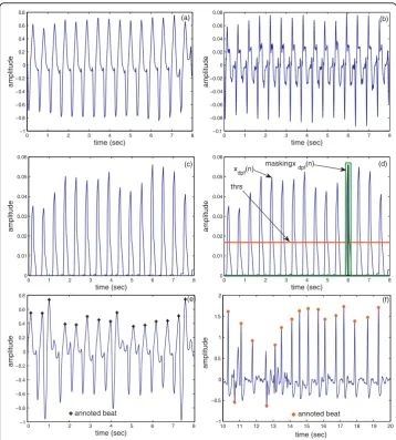
As only the certain classes of VTs and VFs require high-energy shock for treatment, it is necessary to classify the VT and VF according to the heart rate and amplitude, respectively. Since, the heart rate calculation is complicated than the amplitude deter-mination, hence at first we propose a technique to determine the heart rate. The heart rate in bpm is defined as the number of QRS complexes that occur in 60 sec. To determine the heart rate of an ECG signal, first derivative of the ECG signal is utilized. The reason behind the choice of the first derivative of the ECG signal is to utilize the high slope of the QRS complex. Figs. 8(a) and 8(b) show the VT signal and its first derivative. Figure 8(b) illustrates that when QRS complexes occur, correspondingly there is a high value (both in positive and negative part) in the first derivative signal. We consider only the positive part of the first derivative signal. Then this signal is fil-tered to enhance the QRS complexes further. From this filfil-tered signal shown in Figure 8(c), the heart rate is easily calculated. The whole process of determining the heart rate of the ECG signal is described below:
1. First, choose a segmentx(n) of durationLe-second and Nsamples from the
pre-viously saved ECG signal and then perform preprocessing as stated in Section. 2. Calculate the first derivative (xd(n)) of x(n).
x nd( )=x n( )−x n( −1)
The waveform ofxd(n) is shown in Figure 8(b).
3. Keep only the positive part ofxd(n).
x n x n if x n
otherwise
dp
d d
( ) ( ) ( )
;
=⎧⎨ ≥
⎩ 0
0
4. Apply the moving average filter onxdp(n) and findxdpf(n).
xdpf n x n k
k k
( )= ( − )
= =
∑
0where,a=Fs/10 andFsis the sampling frequency. Ifais not an integer, then it is
rounded to the nearest integer value. The waveform ofxdpf(n) is shown in Figure 8(c).
5. Determine the maximum value (C) and the corresponding peak index (I) ofxdpf
(n) and calculate the threshold value (Th) fromC.
C x n
T C
dpf
h =
= ×
max{ ( )}
6. Store the peak index (I) and maskxdpf(n) around this position.
xdpf (I− :I+)=0
where,g=Fs/8; ifgis not an integer, then it is rounded to the nearest integer value.
7. Now, calculate again the maximum value (C) ofxdpf(n) and go through step (vi)
until C goes below theTh.
8. Determine the total number of peaks (Np) those are aboveThand calculateHR.
H N
L bpm
R p
e = ×60
If the heart rate of the VT signal is greater than 180 bpm, then this VT is called the shockable VT. As the decision of shockable or intermediate VT is dependent on the
0 1 2 3 4 5 6 7 8
−1 −0.8 −0.6 −0.4 −0.2 0 0.2 0.4 0.6 0.8 (a) time (sec) amplitude
0 1 2 3 4 5 6 7 8
−0.1 −0.08 −0.06 −0.04 −0.02 0 0.02 0.04 0.06 0.08 time (sec) amplitude (b)
0 1 2 3 4 5 6 7 8
0 0.01 0.02 0.03 0.04 0.05 0.06 time (sec) amplitude (c)
0 1 2 3 4 5 6 7 8
0 0.01 0.02 0.03 0.04 0.05 0.06 time (sec) amplitude (d) thrs
xdpf(n) masking xdpf(n)
−1 −0.8 −0.6 −0.4 −0.2 0 0.2 0.4 0.6 0.8
0 1 2 3 4 5 6 7 8
time (sec)
amplitude
(e)
annoted beat
10 11 12 13 14 15 16 17 18 19 20
−1 −0.5 0 0.5 1 1.5 2 time (sec) amplitude (f) annoted beat
Figure 8Heart rate calculation. ECG waveforms in different stages of the heart rate determination scheme (a) Preprocessed ECG signal,x(n); (b) First derivative,xd(n); (c) Filtered ECG signal,xdpf(n); (d)
Determination of the threshold level and masking ofxdpf(n). (e)-(f) Two episodes are taken to check the
heart rate of the episode, hence, we calculate the total number of QRS beats in a sode. Now, to check the efficiency of the heart rate determination algorithm, two epi-sodes selected are shown in Figs. 8(e)-(f). At first, the total number of QRS beats in these episodes are determined from the annotation. Then, the proposed derivative based heart rate determination algorithm is used to calculate the total number of QRS beats and it is found to be 15 beats for Figure 8(e) and 17 beats for Figure 8(f). In both cases, the total number of QRS complexes obtained by using our algorithm are the same as determined from the annotation. Thus, this heart rate determination method, though simple, may be used to calculate the heart rate of an ECG episode. However, in more complicated cases any standard heart rate determination algorithm re-ported in the literature [38,39] may be adopted to classify the VT. On the other hand, the amplitude of the VF signal is determined by taking the maximum value of the absolute VF signal within a episode. If the amplitude is greater than 200μV, than this VF is called the coarse VF.
Quality Parameters
The quality parameters, we have used for the assessment of algorithms, are sensitivity, speci city, positive predictivity, and accuracy. For ‘VTVF’detection, the first four para-meters are defined by
Sensitivity No of detected VTVF
No of true VTVF
= . " "
. " "
Specificity No of detected nonVTVF
No of true nonVTVF
= . " "
. " "
Positive Predictivity Pos Pred
No of detected VTVF No of ca
( . .)
. " "
.
=
sses classified by algorithm as VTVF" "
Accuracy No of true decisions
No of all decisions
= .
.
For ‘VF’and‘shockable rhythm’detection, the definition of these four quality para-meters contain‘VF’and ‘shockable rhythm’in place of ‘VTVF’, respectively. While cal-culating these four quality parameters to judge the effectiveness of an algorithm, in case of any unsatisfactory results obtained, the values of the respective thresholds were adjusted in order to obtain the best possible results.
Results and Discussion
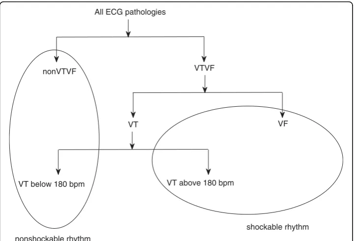
The full classification of different ECG pathologies is shown in Figure 9. To compare our algorithm with other reported algorithms in the literature, our classification approach can be interpreted as three different ECG arrhythmias identification schemes; such as
1. VTVF and nonVTVF
2. VF and nonVF (nonVTVF+VT)
Since the annotated files do not contain enough low-amplitude signals (fine VF), therefore, this type of signal is not addressed in this identification scheme and the VF signals in the shockable rhythms are actually coarse VF. Now, this section is divided into three subsections and each subsection presents the results of each identification scheme.
Detection of VTVF from other arrhythmias
First, we test the separability of our algorithm between the two classes of ECG signals, i.e., ‘VTVF’and‘nonVTVF’against the annotated decisions suggested by the cardiologists in the respective databases. We compare our algorithm with the complexity measure algorithm [10] and the results are shown in Table 1. Comparative results illustrate that our algorithm shows better performance than the complexity measure algorithm. Also notice that the accuracy of the proposed MAV scheme is significantly higher than that of the complexity measure algorithm. Thus our simple and fast algorithm can separate VTVF from nonVTVF with higher specificity and sensitivity simultaneously. In this case, we had to change the threshold value of the CPLX algorithm from that defined in [10] to obtain higher sensitivity.
Detection of VF from other arrhythmias
VF occurs at the clinically crucial stage of human being. As mentioned earlier, while detecting VF from the other arrhythmias in the first stage, we should make the specifi-city high because a low specifispecifi-city may risk patient’s life by generating a false alarm to
nonVTVF
All ECG pathologies
VT VF
VT below 180 bpm VT above 180 bpm
VTVF
shockable rhythm
nonshockable rhythm
Figure 9Classification of different ECG signals. Classification of different types of ECG pathologies.
Table 1 Quality parameters of VTVF detection
Algorithm Quality Parameters for VTVF detection
Sensitivity (%) Specificity (%) Pos. Pred. (%) Accuracy (%)
MAV 93.69 99.39 89.46 99.07
provide a high energy shock as treatment to save his/her life. But our proposed sequential algorithm leads to a high specificity. Quality parameters of our proposed algorithm with some other well-known algorithms are shown in Table 2. It is clear that our algorithm shows higher sensitivity compared to all other algorithms with very good specificity (99.32%). To obtain higher specificity, we had to change the critical threshold parameter of the HILB and PSR methods from that defined in the respective papers. To compare different methods independent of the value of the decision thresh-olds, the critical threshold parameter in the decision stage of the algorithm is varied. By varying the threshold, we can vary specificity and sensitivity as shown in Table 3. This table illustrates that our proposed method performs much better than the other VF detection algorithms.
Detection of shockable rhythms from other arrhythmias
This subsection presents the results of our last identification scheme which classifies the ECG pathologies into two groups: shockable and non-shockable rhythms. To com-pare our algorithm with the reported algorithm in [5], some modifications in the
threshold values are made to accommodate unequal episode lengths (Le). Our
pro-posed algorithm considers Le= 8-s whereLe= 10-s was considered in [5].
Modifica-tions are shown in Table 4. For example, if Count1 < 250 forLe= 10-s, then forLe=
8-s Count1 < 250 10 * 8 orCount1 < 200.
Here, as we concentrate only on the shockable and non-shockable rhythms, some clas-sification errors may not result in detection errors. For example, from Figure 10 we see that a classification error occurs when a VT above 180 bpm is falsely detected as VF in the second stage. Since a VT above 180 bpm (one type of shockable rhythms) is falsely mapped into the VF group, which is also in the class of shockable rhythms, therefore, this classification error does not make any detection error as long as shockable rhythm Table 2 Quality parameters of different VF detection algorithms forLe= 8-s
Algorithm Quality Parameters for VF detection
Sensitivity (%) Specificity (%) Pos. Pred. (%) Accuracy (%)
TCI 94.64 65.08 8.46 66.05
SPEC 41.42 99.57 76.67 97.65
HILB 71.76 98.87 68.41 97.98
PSR 63.69 99.05 69.57 97.88
TCSC 80.19 98.53 65.66 97.96
MAV & EMD 86.49 99.32 81.27 98.90
Table 3 Performance comparison of different algorithms for a fixed specificity and forLe= 8-s
Algorithm Sensitivity if Specificity =
99% 98% 96%
TCI 0.33 0.73 5.73
SPEC 65.2 69.35 74.93
HILB 65.32 84.79 91.58
PSR 62.17 77.53 92.40
TCSC 65.07 84.23 93.94
is our concern. Using the modified threshold values mentioned in Table 4, the results obtained are presented in Table 5. As can be seen, our algorithm performs better than the count [5] algorithm in every index in detecting the shockable rhythms correctly.
Conclusions
A novel method for the identification of life threatening cardiac abnormalities from other arrhythmias has been presented. Performing sequential signal processing, we have detected these cardiac abnormalities with good accuracy. It has been shown that the proposed algorithm based on the MAV parameter and EMD technique can detect the VT plus VF signals correctly from other arrhythmias, and the accuracy level remains higher than that of other reported techniques. The effectiveness of the pro-posed technique has been demonstrated using standard databases over a vast range of
both normal and abnormal ECG records. The MAVindex successfully separates the
VTVF arrhythmias from different types of abnormalities. And the other parameter
NMAV which is calculated using the IMFs of the EMD technique can successfully
Table 4 Modifications in the threshold values proposed in [5] (C1 =Count1,C2 =
Count2,C3 =Count3) Condition
No.
forLe= 10-s forLe= 8-s
1 C1 < 250,C2 > 950 andC1 ×C2/C3 < 210 C1 < 200,C2 > 760 andC1 ×C2/C3 < 168 2 250≤C1 < 400,C2 < 600 andC1 ×C2/C3 <
210
200≤C1 < 320,C2 < 480 andC1 ×C2/C3 < 168
3 C1≥250 &C2 > 950 C1≥200 &C2 > 760
4 C2≥1100 C2≥880
VTVF nonVTVF
VF
VT below 180 VT above 180
VT
VT above 180
VT below 180 VF
nonVTVF
False classification and False detection
False classification and correct detection Correct classification and correct detection
separate VF from VTVF. Finally, a fast and simple heart rate determination technique is used to separate the high rate VT. Consistent results have been obtained by applying our algorithm on different well-known databases namely, MIT-BIH database, CU data-base and MIT-BIH Malignant Ventricular Arrhythmia datadata-base. Determination of the threshold parameters from the training dataset and then their successful application on the test dataset proves that the proposed parameters are universal. Some signal Table 5 Quality parameters for the detection of shockable rhythms usingLe= 8-s
Algorithm Quality parameters for the detection of shockable rhythms Sensitivity (%) Specificity (%) Pos. Pred. (%) Accuracy (%)
MAV & EMD 91.09 99.42 90.71 99.21
Count [5] 88.90 99.29 85.99 98.93
0 1 2 3 4 5
−10 −8 −6 −4 −2 0 2 4 6 8x 10⁻³
0 1 2 3 4 5
−8 −6 −4 −2 0 2 4 6 8 10x 10−3
0 1 2 3 4 5
−3 −2 −1 0 1 2 3x 10
−3
0 1 2 3 4 5
−5 −4 −3 −2 −1 0 1 2 3 4x 10
−3
amplitude
amplitude
amplitude of first IMF
e (n)u x(n)
e (n)l m (n) 1
m (n)12 e (n)u2
h (n)1
e (n)l2
time (sec) time (sec) time (sec) time (sec)
(a)
(b)
(c)
(d)
0 1 2 3 4 5
−8 −6 −4 −2 0 2 4 6x 10⁻³
time (sec)
(e)
amplitude of second IMF
amplitude of residue
Figure 11Illustration of the EMD using an example. (a) The original signalx(n), two envelopeseu(n)
andel(n), and the mean of the envelopem1(n); (b) The first componenth1(n), two envelopeseu2(n) andel2
episodes were very difficult for classification even by expert cardiologists. Accuracy of our proposed technique slightly falls due to these confusing episodes. The algorithm presented here has strong potential to be applied in clinical applications for accurate detection of life threatening cardiac arrhythmias.
Appendix
The steps involved in the EMD technique are described below using an example.
1. Determine the upper envelopeu(n) and the lower envelopel(n). These two
envel-opes are shown in Figure 11(a) along with the original signalx(n).
2. Determine the mean of the envelope, i.e.,m1(n) = [eu(n) +el(n)]/2. The variation
ofm1(n) is displayed in Figure 11(a).
3. Extract the first componenth1(n) using eqn. (3).
4. Ideally,h1(n) should be the first IMF. But, it is observed from Figure 11(b) that
theh1(n) does not satisfy the conditions of an IMF.
5. Now, treath1(n) asx(n) in step (1). Determine the two envelopes fromh1(n) and
the mean of these two envelopes (Figure 11(b)). After subtraction of the mean from theh1(n) a new signalh1(2)(n) is obtained. Now, check the conditions of an
IMF and also calculate the value of SD from eqn. (4), whereh1(1)=h1(n).
6. Continue the process untilh1(k-1)satisfies the conditions of the IMFs. When the
conditions are satisfied, the first IMF is found as shown in Figure 11(c). Now, the first IMF is subtracted from the initial signalx(n).
7. The second IMF (Figure 11(d)) is extracted following the steps (1) to (6) except that the subtracted signal is used instead ofx(n). No further decomposition is per-formed here as we need two IMFs for our analysis. The residue of the EMD is shown in Figure 11(e).
Acknowledgements
This work was supported in part by the National Research Foundation (NRF) of Korea funded by the Korean government (MEST) (No: 2009-0078310).
Author details 1
Department of Electrical and Electronic Engineering, Bangladesh University of Engineering and Technology, Dhaka-1000, Bangladesh.2Department of Biomedical Engineering, Kyung Hee University, Kyungki 446-701, Korea.
Authors’contributions
EM carried out the implementation of the idea, contributed in the development of new characteristic index for discriminating different pathology of signals, collected data from different standard databases for analysis, and drafted the manuscript. SY participated in the design of the study and interpretation of data, and was involved in critically revising the manuscript. MK conceived of the study, and participated in its design, analysis and interpretation of data, defined mathematical index to be used for discriminating arrhythmias, and helped to draft and finalize the manuscript. All authors read and approved the final manuscript.
Competing interests
The authors declare that they have no competing interests.
Received: 19 April 2010 Accepted: 4 September 2010 Published: 4 September 2010
References
1. Amann A, Tratnig R, Unterkofler K:A new ventricular fibrillation detection algorithm for automated external defibrillators.Comput Cardiol2005,32:559-562.
2. Amann A, Tratnig R, Unterkofler K:Detecting ventricular fibrillation by time-delay methods.IEEE Trans Biomed Eng 2007,54:174-177.
3. Barro S, Ruiz R, Cabello D, Mira J:Algorithmic sequential decision-making in the frequency domain for life threatening ventricular arrhythmias and imitative artifacts: a diagnostic system.J Biomed Eng1989,11:320-328. 4. Thakor NV, Zhu YS, Pan KY:Ventricular tachycardia and fibrillation detection by a sequential hypothesis testing
5. Jekova I, Krasteva V:Real Time detection of ventricular fibrillation and tachycardia.Physiol Meas2004,25:1167-1178. 6. Jekova I, Krasteva V, Ménétré S, Stoyanov T, Christov I, Fleischhackl R, Schmid JJ, Didon JP:Bench study of the
accuracy of a commercial AED arrhythmia analysis algorithm in the presence of electromagnetic interferences.
Physiol Meas2009,30:695-705.
7. Gauna SRd, Lazkano A, Ruiz J, Aramendi E:Discrimination between ventricular tachycardia and ventricular fibrillation using the continuous wavelet transform.Computers in Cardiology2004,31.
8. Caswell S, Thompson J, Jenkins J, DiCarlo L:Separation of ventricular tachycardia from ventricular fibrillation using paired unipolar electrograms.Cornputen in Cardiology1996.
9. Arafat MA, Sieed J, Hasan MK:Detection of ventricular fibrillation using empirical mode decomposition and Bayes decision theory.Computers in Biology and Medicine2009,39(11):1051-1057.
10. Zhang XS, Zhu YS, Thakor NV:Detecting ventricular tachycardia and fibrillation by complexity measure.IEEE Trans Biomed Eng1999,46(5).
11. Jekova I, Mitev P:Detection of ventricular fibrillation and tachycardia from the surface ECG by a set of parameters acquired from four methods.Physiol Meas2001,23:629-634.
12. Didon J, Dotsinsky I, Jekova I, Krasteva V:Detection of Shockable and Non-Shockable Rhythms in Presence of CPR Artifacts by Time-Frequency ECG Analysis.Computers in Cardiology2009,36:817-820.
13. Chen S, Thakor NV, Mover MM:Ventricular fibrillation detection by a regression test on the auto-correlation function.Med Biol Eng Comput1987,25.
14. Langer A, Heilman MS, Mower MM, Mirowski M:Considerations in the development of the automatic implantable defibrillator.Med Instrum1976,10.
15. Kuo S, Dillman R:Computer detection of ventricular fibrillation.Comput Cardiol1978.
16. RH Clayton AM, Campbell RWF:Comparison of four techniques for recognition of ventricular fibrillation from the surface ECG.Med Biol Eng Comput1993,31.
17. Heij S, Zeelenberg C:A fast real-time algorithm for the detection of ventricular fibrillation.Comput Cardiol1987, 707-710.
18. Jenkins J, Noh KH, Guezennec A, Bump T, Arzbaecher R:Diagnosis of atrial fibrillation using electrograms from chronic leads: Evaluation of computer algorithms.PACE1988,11:622-631.
19. Ripley KL, Bump TE, Arzbaecher RC:Evaluation of techniques for recognition of ventricular arrhythmias by implanted devices.IEEE Trans Biomed Eng1989,36:618-624.
20. Thakor NV, Natarajan A, Tomaselli G:Multiway sequential hypothesis testing for tachyarrhythmia discrimination.IEEE Trans Biomed Eng1994,41:480-487.
21. Chen SW, Clarkson PM, Fan Q:A robust sequential detection algorithm for cardiac arrhythmia classification.IEEE Trans Biomed Eng1996,43:1120-1125.
22. Lin D, DiCarlo LA, Jenkins JM:Identification of ventricular tachycardia using intracavity ventricular electrograms: Analysis of time and frequency domain patterns.PACE1988,11:1592-1606.
23. Throne RD, Jenkins JM, Winston SA, DiCarlo LA:A comparison of four new time-domain techniques for discriminating monomophic ventricular tachycardia form sinus rhythm using ventricular waveform morphology.
IEEE Trans Biomed Eng1991,38:561-570.
24. Arafat MA, Chowdhury AW, Hasan MK:A simple time domain algorithm for the detection of ventricular fibrillation in electrocardiogram.Signal, Image and Video Processing2009.
25. Werther P, Klotz A, Granegger M, Baubin M, Feichtinger HG, Amann A, Gilly H:Strong corruption of
electrocardiograms caused by cardiopulmonary resuscitation reduces efficiency of two-channel methods for removing motion artefacts in non-shockable rhythms.Resuscitation2009,80(11):1301-1307.
26. Jekova I:Comparison of five algorithms for the detection of ventricular fibrillation from the surface ECG.Physiol Meas2000,21:429-439.
27. Huang NE, Shen Z, Long SR, Wu MC, Shih HH, Zheng Q, Yen NC, Tung CC, Liu HH:The empirical mode decomposition and hilbert spectrum for nonlinear and nonstationary time series analysis.Proc R Soc Lond1998, 454.
28. Massachusetts Institute of Technology, MIT-BIH arrhythmia database.[http://www.physionet.org/physiobank/ database/mitdb].
29. Massachusetts Institute of Technology, CU database.[http://www.physionet.org/physiobank/database/cudb]. 30. Massachusetts Institute of Technology, MIT-BIH Malignant Ventricular Fibrillation database.[http://www.physionet.
org/physiobank/database/vfdb].
31. Jones SA:ECG NotesPhiladelphia: Nursing: Lisa Deitch 2005.
32. Amann A, Tratnig R, Unterkofler K:Reliability of old and new ventricular fibrillation detection algorithms for automated external defibrillators.Biomed Eng Online2005,4(60) [http://www.biomedcentral.com/content/pdf/1475-925x-4-60.pdf].
33. filtering.m.[https://homepages.fhv.at/ku/karl/VF/filtering.m].
34. Junsheng C, Dejie Y, Yu Y:Research on the intrinsic mode function (IMF) criterion in EMD method.Mechanical Systems and Signal Processing2006,20(4):817-824.
35. Flandrin P:Time-Frequency/Time-Scale AnalysisAcademic Press 1999.
36. Gregory JA:Shape preserving spline interpolation.Computer-Aided Design1986,18:53-57.
37. Sharpley RC, Vatchev V:Analysis of the Intrinsic Mode Functions.Constructive Approximation2006,24:17-47. 38. Afonso VX, Tompkins WJ:ECG Beat Detection Using Filter Banks.IEEE Transactions on Biomedical Engineering1999,
46(12):192-202.
39. Arafat MA, Hasan MK:Automatic Detection of ECGWave Boundaries using Empirical Mode Decomposition.Proc ICASSP2009, 461-464.
doi:10.1186/1475-925X-9-43