S O F T W A R E
Open Access
CPMCGLM: an R package for
p
-value
adjustment when looking for an optimal
transformation of a single explanatory
variable in generalized linear models
Benoit Liquet
1,2†and Jérémie Riou
3*†Abstract
Background: In medical research, explanatory continuous variables are frequently transformed or converted into categorical variables. If the coding is unknown, many tests can be used to identify the “optimal” transformation. This common process, involving the problems of multiple testing, requires a correction of the significance level.
Liquet and Commenges proposed an asymptotic correction of significance level in the context of generalized linear models (GLM) (Liquet and Commenges, Stat Probab Lett 71:33–38, 2005). This procedure has been developed for dichotomous and Box-Cox transformations. Furthermore, Liquet and Riou suggested the use of resampling methods to estimate the significance level for transformations into categorical variables with more than two levels (Liquet and Riou, BMC Med Res Methodol 13:75, 2013).
Results: CPMCGLMprovides to users both methods ofp-value adjustment. Futhermore, they are available for a large set of transformations.
This paper aims to provide insight the user an overview of the methodological context, and explain in detail the use of theCPMCGLMR package through its application to a real epidemiological dataset.
Conclusion: We present here theCPMCGLM Rpackage providing efficient methods for the correction of type-I error rate in the context of generalized linear models. This is the first and the only available package inRproviding such methods applied to this context.
This package is designed to help researchers, who work principally in the field of biostatistics and epidemiology, to analyze their data in the context of optimal cutoff point determination.
Keywords: R package, Generalized linear model, Resampling,p-value adjustment, Multiple testing, Union intersection test, Optimal cutoff point determination
Background
In applied statistics, statistical models are widely used to assess the relationship between an explanatory and a dependent variable. For instance, in epidemiology, it is common for a study to focus on one particular risk factor. Scientists may wish to determine whether the potential risk factor actually affects the risk of a disease, a biological
*Correspondence:[email protected]
†Benoit Liquet and Jérémie Riou contributed equally to this work.
3MINT UMR INSERM 1066, CNRS 6021, Université d’Angers, UFR Santé, 16
Boulevard Davier, 49085 Angers Cedex, France
Full list of author information is available at the end of the article
trait, or another outcome. In this context, statisticians use regression models with an outcome Y, a risk factor X (continuous variable of interest) and q − 1 adjust-ment variables. In clinical and psychological research, the usual approach involves dichotomizing the continuous variable, whereas, in epidemiological studies, it is more usual to create several categories or to perform continu-ous transformations [1]. It is important to note that the categorization of a continuous predictor can only be jus-tified when threshold effects are suspected. Furthermore, when the assumption of linearity is found to be untenable,
a fractional polynomial (FP) transformation should always be favoured.
For instance, let us consider a categorical transfor-mation of X. When the optimal set of cutoff points is unknown, the subjectivity of the choice of this set may lead to the testing of more than one set of values, to find the “optimal” set. For each coding, the nullity of the coeffi-cient associated with the new coded variable is tested. The coding finally selected is that associated with the small-est p-value. This practice implies multiple testing, and an adjustment of the p-value is therefore required. The CPMCGLMpackage [2] can be used to adjust thep-value in the context of generalized linear models (GLM).
We present here the statistical context, and the vari-ous codings available in this Rpackage. We then briefly present the available methods for type-I error correc-tion, before presenting an example based on the PAQUID cohort dataset.
Implementation Statistical setting Generalized linear model
Let us consider a generalized linear model withq explana-tory variables [3], in whichY = (Y1,. . .,Yn)is observed and the Yi’s are all identically and independently dis-tributed with a probability density function in the expo-nential family, defined as follows:
fYi(Yi,θi,φ)=exp
Yiθi−b(θi)
a(φ) +c(Yi,φ)
;
withE[Yi]=μi=b(θi),Var[Yi]=b(θi)a(φ)and where a(·),b(·), andc(·)are known and differentiable functions. b(·) is three times differentiable, and its first derivative b(·)can be inverted. Parameters(θi,φ)belong to⊂R2, whereθi is the canonical parameter andφ is the disper-sion parameter. TheCPMCGLMpackage allows the use of linear, Poisson, logit and probit models. The specifications of the model are defined with formula, family and link arguments, as aglm()function.
In this context, the main goal is evaluating the associa-tion between the outcomeYiand an explanatory variable of interestXi, adjusted on a vector of explanatory variables Zi. The form of the effect ofXi is unknown, so we may considerKtransformations of this variableXi(k)=gk(Xi) withk=1,. . .,K.
For instance, if we transform a continuous variable into a categorical variable withmkclasses, thenmk−1 dummy variables are defined from the function gk(·): Xi(k) = gk(Xi)=
Xi1(k),. . .,Xmk−1 i (k)
.mkdifferent levels of the categorical transformation are possible.
The model for one transformationkcan be obtained by modeling the canonical parameterθias:
θi(X,Z,k)=γZi+βkXi(k), 1≤i≤n;
where Zi =
1,Zi1,. . .,Ziq−1,γ = (γ0,. . .,γq−1)T is a vector of q regression coefficients, andβk is the vector
of coefficients associated with the transformationkof the variableXi.
Multiple testing problem
We consider the problem of testing
H0,k :βk=0 against H1,k:βk=0,
simultenaously for allk∈ {1,. . .,K}. For each transforma-tionk, one test scoreTk(Y)is obtained for the nullity of the vectorβk[4]. We ultimately obtain a vector of
statis-tics T = (T1(Y),. . .,TK(Y)). Introduce the associated p-value as
pk(y)=Pβk=0(|Tk(Y)| ≥ |Tk(y)|), 1≤k≤K,
whereyis the realization ofY.
Significance level correction
To cope with the multiplicity problem, we aim at testing [5]:
H0 :
K
k=1
H0,k against H1 : K
k=1
H1,k,
by which we mean thatXhas an effect onYif and only if at least one transformation ofXhas an effect onY. A natural approach is then to consider the maximum of the indi-vidual test statisticsTk(Y), or, equivalently, the minimum of the individualp-valuespk(Y), leading to the following p-values:
pmaxT(y)=PY∼P0
TmaxT(Y)≥TmaxT(y)
,
whereP0denote the distribution ofY under the null and TmaxT(·)=max1≤k≤K{|Tk(·)|}, or
pminP(y)=PY∼P0
pminP(Y)≤pminP(y) ,
wherepminP(·)=min1≤k≤K
pk(·)
.
Moreover, ifXhas an effect onY (e.g.H0is rejected), the best coding corresponds to the transformation k which obtains the highest individual test statistic realiza-tionTk(y), or, equivalently, the smallest individualp-value realizationpk(y).
Bonferroni method
The first method available in this package is the Bon-ferroni method. This is the most widely used correc-tion method in applied statistics. It has been described by several authors in various applications [6–10]. The Bonferroni method rejectsH0at levelα∈[ 0, 1] if
pminP(y)≤ α
whereKis related to the total number of tests performed by the user. However, this method is conservative, particu-larly when the correlation between test results is high and the number of transformations is high.
Exact method
The second method proposed in this package is the asymptotic exact correction developed by Liquet and Commenges for generalized linear models [11, 12]. This method is valid only for binary transformations, frac-tional polynomial transformations with one degree (i.e. FP1) and Box-Cox transformations. It is based on the joint asymptotic distribution of the test statistics under the null. Indeed, thep-valuepmaxTcan be calculated as follows:
pmaxT(y) = 1−PY∼P0
TmaxT(Y) <TmaxT(y)
= 1−PY∼P0(T1(Y) <T
maxT(y);. . .;
TK(Y) <TmaxT(y)).
We then calculated the probability PY∼P0
T1(Y) < TmaxT(y);. . .;TK(Y) < TmaxT(y) by numerical integra-tion of the multivariate Gaussian density (e.g., the asymp-totic joint distribution of (Tk)1≤k≤K). Several programs have been written to solve this multiple integral. In this package, we used the method developed by Genz and Bretz in 2009 [13], available in the mvtnorm R package [14].
Minimum p-value procedure
The approach based on pminP, called the minimum p-value procedure, allows to combine statistical tests for different distributions. It is therefore possible to combine dichotomous, Box-Cox, fractional polynomial and trans-formations into categorical variables with more than two levels. However, the distribution ofpminPis unknown and we use resampling-based methods. These procedures take into account the dependence structure of the tests for evaluation of the significance level of the minimum p-value procedure. These procedures can therefore be used for all kinds of coding.
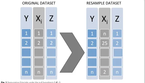
Permutation test procedure The first resampling-based method is a permutation test procedure. This procedure is used to build the reference distribution of statistical tests based on permutations. From a theoretical point of view, the statistical test procedures are developed by consider-ing the null hypothesis to be true, i.e. in our context, under the null hypothesis,Xihas no impact onY. Under the null hypothesis, if the exchangeability assumption is satisfied [15–20], then resampling can be performed based on the permutation ofXithe variable of interest in our dataset. The procedure proposed by Liquet and Riou could be summarized by the following algorithm [6]:
1 Apply the minimump-value procedure to the
original data for theK transformations considered.
We notepminthe realization of the minimum of the
p-value;
2 UnderH0,k,Xihas no effect on the response variable
Y, and a new dataset is generated by permuting the
Xivariable in the initial dataset. This procedure is
illustrated in the following Fig.1;
3 GenerateB new datasetss∗b,b= {1, ...,B}by
repeating step 2B times;
4 For each new dataset, apply the minimump-value
procedure for the transformation considered. We
notep∗minb the smallestp-value for each new dataset.
5 Thep-value is then approximated by:
pminP= 1 B
B
b=1 I
p∗bmin<pmin
,
whereI{·}is an indicator function.
This procedure can be used to control for the type-I error.
Parametric bootstrap procedure The second resampling-based method is the parametric bootstrap procedure, which yields an asymptotic reference distribution. This procedure makes it possible to control for type-I error with fewer assumptions [21]. This procedure is summa-rized in the following algorithm [6]:
1 Apply the minimump-value procedure to the
original data for theK transformations considered.
We notepminthe realization of the minimum of the
p-value;
2 Fit the model under the null hypothesis, using the
observed data, and obtainγˆ, the maximum
likelihood estimate (MLE) ofγ;
3 Generate a new outcomeYi∗for each subject from
the probability measure defined underH0,k.
4 Repeat this for all the subjects to obtain a sample denoteds∗= {Yi∗,Zi,Xi}
5 GenerateB new datasetss∗b,b=1,. . .,Bby
repeating step 3B times ;
6 For each new dataset, apply the minimump-value
procedure for the transformation considered. We
notep∗minb the smallestp-value for each new dataset.
7 Thep-value is then approximated by:
pminP= 1 B
B
b=1 I
p∗bmin<pmin
.
Codings
Fig. 1Permutation Principle under the null hypothesisH0,k
Dichotomous coding
Dichotomous coding is often used in clinical and psy-chological research, either to facilitate interpretation, or because a threshold effect is suspected. In regression models with multiple explanatory variables, it may be seen as easier to interpret the regression coefficient for a binary variable than to understand a one-unit change in the continuous variable. In this context, dichoto-mous transformations of the variable of interest X are defined as:
X(k)=
1 if X≥ck; 0 if X<ck,
whereckdenotes the cutoff value for the transformationk (1≤k≤K).
In this R package, the dicho argument of the CPMCGLM() function allows the definition of desired cutoff points based on quantiles in avector. An example of thedichoargument is provided below:
Code 1: Definition of 3 dichotomous transformations
dicho <- c( 0.2, 0.5, 0.7)
In this example, the user wants to try three dichoto-mous transformations of the variable of interest. For the first transformation, the cutoff point is the second decile; for the second, it is the median, and for the third, the seventh decile. The user can also opt to use our quantile-based method. The choice of this method leads to use of
the nb.dicho argument. This argument makes it pos-sible to use a quantile-based method, by entering the desired number of transformations. If the user asks for three transformations, the program uses the quartiles as cutoff points. If two transformations are requested, the program uses the terciles, and so on. This argument is also defined as follows.
Code 2: Three dichotomous transformations nb.dicho <- 3
It is important to note that only one of these argu-ments (dichoandnb.dicho) can be used in a given CPMCGLM()function.
Coding with more than two classes
In epidemiology, it is usual to create several categories, often four or five. These transformations into categorical variables are defined as follows:
X(k)= ⎧ ⎪ ⎪ ⎪ ⎪ ⎪ ⎪ ⎨ ⎪ ⎪ ⎪ ⎪ ⎪ ⎪ ⎩
m−1 ifX≥ckm−2; ..
. ...
j if ckj >X≥ckj−1; ..
. ... 0 if X<ck0,
whereckjdenotes thejthcutoff point(0≤j≤m−2), for
the transformationk(1≤k≤K).
using quantiles. This argument must take the form of a matrix, with a number of columns matching the maxi-mum number of cutoff points used in almost all trans-formations, and a number of rows corresponding to the number of transformations tried. An example of this argu-ment definition is presented below:
Code 3: Four categorical transformations
categ <- matrix(NA, nrow=4, ncol=3) categ[1,1:2] <- c(0.3, 0.7)
categ[2,1:2] <- c(0.4, 0.6)
categ[3,1:3] <- c(0.25, 0.5, 0.75) categ[4,1:3] <- c(0.4, 0.6, 0.8)
In this example, the user will realize four transforma-tions. Two involve transformation into three classes, and two into four classes. It is important to note that binary transformations could not be defined here. The maximum number of cutoff points used in almost all transformations is three. The matrix therefore has the following dimen-sions:(4×3). For the first transformation, we will define a transformation into a three-class categorical variable with the third and seventh deciles as cut-points, and so on for the other transformations.
The user could also use a quantile-based method to define the transformations. In this case, the user would need to define the number of categorical transformations in thenb.categ argument. If two transformations are requested, then this method will create a two-class cat-egorical variable using the terciles as cutoff points, and a three-class categorical variable using the quartiles as cutoff points. If the user asks for three transformations, the first and second transformations remain the same, and the program creates another categorical variable with four classes based on the quintiles, and so on. For four transformations, the argument is defined inRas follows:
Code 4: Four categorical transformations
nb.categ <- 4
However, users may also wish to define their own set of thresholds. For this reason, the function also includes the argumentcutpoint, which can be defined on the basis of true values for the transformations desired. This argu-ment is a matrix, defined as the arguargu-mentcateg. The dif-ference between this argument and that described above is that it is possible to define dichotomous transformations for this argument and quantiles are not used.
Code 5: Three categorical transformations
cutpoint <- matrix(NA, nrow=3, ncol=3) cutpoint[1,1] <- c(20)
cutpoint[2,1:2] <- c(15, 25) cutpoint[3,1:3] <- c(10, 20, 30)
Box-Cox transformation
Other transformations are also used, including Box-Cox transformations in particular, defined as follows [22]:
X(k)=
λ−1k (Xλk−1) if λk>0 logX if λk=0,
This family of transformations incorporates many tradi-tional transformations:
• λk= 1.00: no transformation needed; produces
results identical to original data
• λk= 0.50: square root transformation
• λk= 0.33: cube root transformation
• λk= 0.25: fourth root transformation
• λk= 0.00: natural log transformation
• λk= -0.50: reciprocal square root transformation
• λk= -1.00: reciprocal (inverse) transformation
Theboxcoxargument is used to define Box-Cox trans-formations. This argument is a vector, and the values of its elements denote the desired λk. An example of the boxcoxargument for a reciprocal transformation, a nat-ural log transformation, and a square root transformation is provided below:
Code 6: Three Box-Cox transformations
boxcox <- c( -1, 0, 0.5 )
Fractional polynomial transformation
Royston et al. showed that traditional methods for ana-lyzing continuous or ordinal risk factors based on cate-gorization or linear models could be improved [23, 24]. They proposed an approach based on fractional polyno-mial transformation. Let us consider generalized linear models with canonical parameters defined as follows:
θi(X,Z)=γZi+βXi, 1≤i≤n;
whereZi =
1,Zi1,. . .,Ziq−1
,γ = (γ0,. . .,γq−1)T is a vector ofqregression coefficients, andβis the coefficient associated with theXivariable.
Consider the arbitrary powersa1 ≤ . . . ≤ aj ≤ . . . ≤ am, with 1≤j≤m, anda0=0.
If the random variable X is positive, i.e. ∀i ∈
{1,. . .,n},Xi >0, then the fractional polynomial transfor-mation is defined as:
θm
i (X,Z,ξ,a)=γZi+ m
j=0
ξjHj(Xi),
where for 0≤ j ≤ mξjis the coefficient associated with the fractional polynomial transformation:
Hj(Xi)=
Xi(aj) ifaj=aj−1 Hj−1(Xi)ln(Xi) ifaj=aj−1
However, if non-positive values ofXcan occur, a prelim-inary transformation ofXto ensure positivity is required. The solution proposed by Royston and Altman is to choose a non-zero originζ <Xiand to rewrite the canon-ical parameter of the model for fractional polynomial transformation as follows:
θm
i (X,Z,ξ,a)=γZi+ m
j=0
ξjHj(Xi−ζ),
ζ is set to the lower limit of the rounding interval of samples values for the variable of interest.
Royston and Altman suggested usingmpowers from a predefined setP[25]:
P= {−max(3,m);. . .;−2;−1;−0.5; 0; 0.5; 1; 2;. . .; max(3,m)}.
TheFPargument is used to define these transformations. This argument is a matrix. The number of rows corre-spond to the number of transformations tested, and the number of columns is the maximum number of degrees tested for a single transformation. An example of theFP argument:
Code 7: fractional polynomial transformations
# Three transformations of degrees 1, 4 and 2.
FP <- matrix(NA,ncol=4,nrow=3) FP[1,1] <- -2
FP[2,] <- c(0.5,1,-0.5,2) FP[3,1:2] <- c(-0.5,1)
In this example, the user performs three transforma-tions of the variable of interest. The first is a fractional polynomial transformation with one degree and a power of −2. The second transformation is a fractional poly-nomial transformation with four degrees and powers of 0.5, 1,−0.5, and 2. The third transformation is a fractional polynomial transformation with two degrees and powers of−0.5, and 1.
Motivating example
We revisited the example presented in the article of Liquet and Commenges in 2001 based on the PAQUID database [11], to illustrate the use of theCPMCGLMpackage, in the context of logistic regression.
PAQUID database
PAQUID is a longitudinal, prospective study of individ-uals aged at least 65 years on December 31, 1987 liv-ing in the community in France. These residents live in two administrative areas in southwestern France. This elderly population-based cohort of 3111 community res-idents aimed to identify the risk factors for cognitive decline, dementia, and Alzheimer’s disease. The data were obtained in a nested case-control study of 311 subjects from this cohort (33 subject with dementia and 278 controls).
Scientific aims
The analysis focused on the influence of HDL(high-density lipoprotein)-cholesterol on the risk of dementia. We considered the variables age, sex, education level, and wine consumption as adjustment variables. Bonarek et al initially considered HDL-cholesterol as a contin-uous variable [26]. Subsequently, to facilitate clinical interpretation, they decided to transform this variable into a categorical variable with different thresholds, and different numbers of classes. This strategy implied the use of multiple models, and multiple testing. A correction of type-I error taking into account the various transfor-mations performed was therefore required to identify the best association between dementia and HDL-cholesterol.
Methods
We applied the various types of correction method described in this article to correct the type-I error rate in the model defined above. These corrections are easy to apply with theCPMCGLMpackage. The following syntax provided the desired results for one categorical coding, three binary codings, one Box-Cox transformation withλ=0, and one fractional polynomial transformation with two degrees and powers of -0.5, and 1:
Code 8: PAQUID Example
# Load Package require(CPMCGLM)
# fractional polynomial definition FP1 <- matrix(NA,ncol=2,nrow=1) FP1[1,] <- c(-0.5,1)
# Call of CPMCGLM function fit <- CPMCGLM( formula=
DEM1_8~ HDL_8+ as.factor(SEXE) + AGE8+ as. factor(certif) + as.factor(VIN0),family ="binomial", link="logit",data=PAQUID, varcod="HDL_8", N=10000,boxcox=c(0),nb. dicho=3,nb.categ=1,FP=FP1)
# print fit fit
# summary fit summary(fit)
By using the "dicho", and "categ" arguments, the function could also be used as follows, for exactly the same analysis:
Code 9: PAQUID Example
# Load Package require(CPMCGLM)
# Definition of categorical transformations in a matrix
categ.mat <- matrix(NA, nrow=1, ncol=3) categ.mat[1,] <- c(0.25,0.5,0.75) # Call of CPMCGLM function
fit1 <- CPMCGLM(formula=
DEM1_8 ~ HDL_8+as.factor(SEXE)+ AGE8 +as. factor(certif)+as.factor(VIN0), family= "binomial", link="logit",data=PAQUID, varcod="HDL_8",N=10000,boxcox=c(0), dicho=c(0.25,0.5,0.75), categ=categ.mat ,FP=FP1)
# print fit fit1
Results
In R software, the results obtained with the CPMCGLM package described above are summarized as follows:
Code 10: Output of the CPMCGLM() function - PAQUID Example > fit
Call: CPMCGLM(formula = DEM1_8 ~ HDL_8 + as .factor(SEXE) + AGE8 + as.factor(certif ) + as.factor(VIN0), family = "binomial ", link = "logit", data = PAQUID, varcod = "HDL_8", nb.dicho = 3, nb. categ = 1, boxcox = c(0), N = 10000,FP= FP1)
Generalize Linear Model Summary Family: binomial
Link: logit
Number of subject: 311
Number of adjustment variable: 6
Resampling N: 1000
Best coding Method: Dichotomous transformation Value of the order quantile cutoff points: 0.75 Value of the quantile cutoff points: 1.615
Corresponding adjusted p value:
Adjusted pvalue naive 0.0010 Bonferroni 0.0051 bootstrap 0.0030 permutation 0.0030 exact: Correction not available for these codings
We can also use the summary function for the main results, which are described as follows for this specific result:
Code 11: Summary for output of the CPMCGLM() function -PAQUID Example
> summary(fit)
Summary of CPMCGLM Package
Best coding Method: Quantile Value of the quantile cutoff points: 0.75
Corresponding adjusted pvalue:
Adjusted pvalue naive 0.0010 Bonferroni 0.0051 bootstrap 0.0030 permutation 0.0030 exact: Correction not available for these codings
As we can see, for this example, the best coding was obtained for the logistic regression with dichotomous coding of the HDL-cholesterol variable. The cutoff point retained for this variable was the third quartile. Exact correction was not available for this application, due to the use of transformation into categorical variables with more than two classes. Resampling methods gave simi-lar results, and both the resampling methods tested were more powerful than Bonferroni correction. In conclusion, the correction of type-I error is required. Naive correction
is not satisfactory, and resampling methods seem to give the best results forp-value correction in this example.
Conclusion
We present hereCPMCGLM, anRpackage providing effi-cient methods for the correction of type-I error rate in the context of generalized linear models. This is the only avail-able package inRproviding such methods applied to this context. We are currently working on the generalization of these methods to proportional hazard models, which we will make available as soon as possible in theCPMCGLM package.
In practice, it is important to correct the multiplicity on all the codings that have been tested. Indeed, if this is not done, the type-I error is not controlled, and then it is possible to obtain some false positive results.
To conclude, this package is designed to help researchers who work principally in epidemiology to analyze with riguor their data in the context of optimal cutoff point determination.
Availability and requirements Project name:CPMCGLM
Project home page: https://cran.r-project.org/web/ packages/CPMCGLM/index.html
Operating system(s):Platform independent Programming language:R
Other requirements:R 2.10.0 or above License:GPL-2
Any restrictions to use by non-academics:none
Abbreviations
FP: Fractional polynomial; GLM: Generalized linear model; HDL: High-density lipoprotein; MLE: Maximum likelihood estimate; PAQUID: Personnes agées QUID
Acknowledgements
We thank Luc Letenneur for his help on the PAQUID dataset, and Marine Roux for her help during the review process.
Funding
No funding was obtained for this study.
Availability of data and materials
The data that are used to illustrate this package are available from Centre de recherche INSERM U1219, Université de Bordeaux, ISPED but restrictions apply to the availability of these data, which were used under license for the current study, and so are not publicly available. Data are however available from the authors upon reasonable request and with permission of Centre de recherche INSERM U1219 Université de Bordeaux, ISPED.
Authors’ contributions
BL and JR developed the methodology, the R code, performed the analysis on the dataset as well as wrote the manuscript. Both authors read and approved the final manuscript.
Ethics approval and consent to participate
Consent for publication
Not applicable.
Competing interests
The author(s) declared no potential conflicts of interest with respect to the research, authorship, and/or publication of this article.
Publisher’s Note
Springer Nature remains neutral with regard to jurisdictional claims in published maps and institutional affiliations.
Author details
1Université de Pau et Pays de l’Adour, UFR Sciences et Techniques de la Cote
Basque-Anglet UMR CNRS 5142, Allée du Parc Montaury, 64600 Anglet, France. 2ARC Centre of Excellence for Mathematical and Statistical Frontiers and
School of Mathematical Sciences at Queensland University of Technology, Brisbane, Australia.3MINT UMR INSERM 1066, CNRS 6021, Université d’Angers, UFR Santé, 16 Boulevard Davier, 49085 Angers Cedex, France.
Received: 11 March 2018 Accepted: 18 March 2019
References
1. Royston P, Altman DG, Sauerbrei W. Dichotomizing continuous predictors in multiple regression: a bad idea. Stat Med. 2006;25(1):127–41. 2. Riou J, Diakite A, Liquet B. CPMCGLM: Correction of thePvalue After
Multiple Coding. 2017. R package.http://CRAN.R-project.org/package= CPMCGLM.
3. McCullagh P, Nelder JA. Generalized Linear Models, Second Edition. Chapman & Hall/CRC Monographs on Statistics & Applied Probability. London: Taylor & Francis; 1989.
4. Rao CR. Large sample tests of statistical hypotheses concerning several parameters with applications to problems of estimation. In: Mathematical Proceedings of the Cambridge Philosophical Society, vol. 44. Cambridge University Press; 1948. p. 50–57.
5. Berger RL. Multiparameter hypothesis testing and acceptance sampling. Technometrics. 1982;24(4):295–300.
6. Liquet B, Riou J. Correction of the significance level when attempting multiple transformations of an explanatory variable in generalized linear models. BMC Med Res Methodol. 2013;13(1):75.
7. Delorme P, Micheaux PL, Liquet B, Riou J. Type-ii generalized family-wise error rate formulas with application to sample size determination. Stat Med. 2016;35(16):2687–714.
8. Simes R. An improved Bonferroni procedure for multiple tests of significance. Biometrika. 1986;73(3):751–4.
9. Worsley KJ. An improved bonferroni inequality and applications. Biometrika. 1982;69:297–302.
10. Hochberg Y. A sharper bonferroni procedure for multiple test procedure. Biometrika. 1988;75:800–2.
11. Liquet B, Commenges D. Correction of thep-value after multiple coding of an explanatory variable in logistic regression. Stat Med. 2001;20: 2815–26.
12. Liquet B, Commenges D. Computation of thep-value of the minimum of score tests in the generalized linear model, application to multiple coding. Stat Probab Lett. 2005;71:33–38.
13. Genz A, Bretz F. Computation of Multivariate Normal and T Probabilities. Lecture Notes in Statistics. Heidelberg: Springer; 2009.
14. Genz A, Bretz F, Miwa T, Mi X, Leisch F, Scheipl F, Hothorn T. mvtnorm: Multivariate Normal and T Distributions. 2016. R package version 1.0-5.
http://CRAN.R-project.org/package=mvtnorm.
15. Romano JP. On the behavior of randomization tests without a group invariance assumption. J Am Stat Assoc. 1990;85:686.
16. Xu H, Hsu JC. Applying the generalized partitioning principle to control the generalized familywise error rate. Biom J. 2007;49(1):52–67. 17. Kaizar EE, Li Y, Hsu JC. Permutation multiple tests of binary features do
not uniformly control error rates. J Am Stat Assoc. 2011;106(495):1067–74. 18. Commenges D, Liquet B. Asymptotic distribution of score statistics for
spatial cluster detection with censored data. Biometrics. 2008;64(4): 1287–9.
19. Commenges D. Transformations which preserve exchangeability and application to permutation tests. J Nonparametric Stat. 2003;15(2):171–85.
20. Westfall PH, Troendle JF. Multiple testing with minimal assumptions. Biom J. 2008;50(5):745–55.
21. Good PI. Permutation Tests. New York: Springer; 2000. 22. Box GE, Cox DR. An analysis of transformations. J R Stat Soc Ser B
Methodol. 1964211–52.
23. Royston P, Altman DG. Regression using fractional polynomials of continuous covariates: parsimonious parametric modelling. Appl Stat. 1994429–67.
24. Royston P, Ambler G, Sauerbrei W. The use of fractional polynomials to model continuous risk variables in epidemiology. Int J Epidemiol. 1999;28(5):964–74.
25. Royston P, Altman DG. Approximating statistical functions by using fractional polynomial regression. J R Stat Soc Ser D (The Stat). 1997;46(3): 411–22.
26. Bonarek M, Barberger-Gateau P, Letenneur L, Deschamps V, Iron A, Dubroca B, Dartigues J. Relationships between cholesterol,