Methods for confidence interval estimation of a ratio parameter with application to location quotients

Open Access

Research article

Methods for confidence interval estimation of a ratio parameter

with application to location quotients

Joseph Beyene*

_{and Rahim Moineddin}

Address: 1_{Department of Public Health Science, University of Toronto, Toronto, Ontario, Canada,} 2_{The Research Institute, Hospital for Sick} Children, Toronto, Ontario, Canada and 3_{Department of Family and Community Medicine, Research Program, University of Toronto, Toronto,} Ontario, Canada

Email: Joseph Beyene* - [email protected]; Rahim Moineddin - [email protected] * Corresponding author

Abstract

Background: The location quotient (LQ) ratio, a measure designed to quantify and benchmark the degree of relative concentration of an activity in the analysis of area localization, has received considerable attention in the geographic and economics literature. This index can also naturally be applied in the context of population health to quantify and compare health outcomes across spatial domains. However, one commonly observed limitation of LQ is its widespread use as only a point estimate without an accompanying confidence interval.

Methods: In this paper we present statistical methods that can be used to construct confidence intervals for location quotients. The delta and Fieller's methods are generic approaches for a ratio parameter and the generalized linear modelling framework is a useful re-parameterization particularly helpful for generating profile-likelihood based confidence intervals for the location quotient. A simulation experiment is carried out to assess the performance of each of the analytic approaches and a health utilization data set is used for illustration.

Results: Both the simulation results as well as the findings from the empirical data show that the different analytical methods produce very similar confidence limits for location quotients. When incidence of outcome is not rare and sample sizes are large, the confidence limits are almost indistinguishable. The confidence limits from the generalized linear model approach might be preferable in small sample situations.

Conclusion: LQ is a useful measure which allows quantification and comparison of health and other outcomes across defined geographical regions. It is a very simple index to compute and has a straightforward interpretation. Reporting this estimate with appropriate confidence limits using methods presented in this paper will make the measure particularly attractive for policy and decision makers.

Background

Effects in comparative analysis are commonly expressed as ratios. One such example is the Location Quotient (LQ), a ratio statistic widely used by geographers,

econo-mists and regional planners to measure the degree of rel-ative concentration of an activity on a map [1,2]. The LQ, which is sometimes referred to as concentration ratio, allows the comparison of an area's share of a specific activ-Published: 12 October 2005

BMC Medical Research Methodology 2005, 5:32 doi:10.1186/1471-2288-5-32

Received: 17 June 2005 Accepted: 12 October 2005 This article is available from: http://www.biomedcentral.com/1471-2288/5/32

© 2005 Beyene and Moineddin; licensee BioMed Central Ltd.

ity with the share of a base aggregate. Furthermore, LQ can produce a rough benchmark in the analysis of localization in an area [3].

In general, statistical inference is more complicated for a ratio of parameters than measures that are expressed as linear combinations. In epidemiological studies, for example, association of risk factors with occurrence of dis-ease in a given study population can be quantified using absolute measures such as the risk difference or by apply-ing relative measures such as the relative risk or odds ratio [4]. Both the relative risk and the odds ratio require more caution from an inferential point of view than the simple risk difference. One of the difficulties in dealing with ratios arises in computing variance estimators.

Despite its popularity as a relative measure, the location quotient is often interpreted and reported primarily as a point estimate without an accompanying measure of pre-cision. However, statistical reasoning and any inferential conclusion one may draw from a sample statistics should reflect uncertainty inherent in the estimation procedure, and appropriate methods that allow proper interpretation of study findings should be used. One way of proper anal-ysis is to construct confidence limits around the sample estimates.

The objective of this paper is to present a number of alter-native approaches that can be used to construct confi-dence limits for measures involving ratios quantities in general and the location quotient in particular.

Methods

A location quotient is a way of measuring the relative con-tribution of one specific area to the whole for a given out-come. Let x_i and n_i denote the outcome and population size of the ith _{area, respectively. Similarly, let x} = ∑_x

i and n = ∑n_i be the outcome and population size of the whole, respectively. The location quotient for the ith _{area is}

defined as

Depending upon the health outcome under study, the random variables in equation (1) may have different scales of measurements including continuous, binary or counts.

The interpretation of the LQ is as follows: (1) LQ_i = 1 which indicates that the outcome in the specific region is at the same level as the aggregate, (2) LQ_i > 1 indicating that the specific region is at a level greater than expected,

and (3) LQ_i < 1 which would indicate that the regional measure is at a level that is less than expected.

To fix notations, suppose interest lies in making inference

about a ratio parameter . In this paper, our focus is

on confidence interval estimation of θ. Let be an

estimate of θ, where the mean parameters for the esti-mates are given by E( ) = α and E( ) = β, respectively. Furthermore, let the estimated variance-covariance matrix

of the estimators ( , ) be given by

where V₁₁ and V₂₂ represent the variance of and , respectively, and V12 = V21denote the covariance between

and .

For the location quotient described in equation (1),

, .

It can easily be shown that

where the parameter p_i denotes the true incidence rate in the ith _{area [5].}

Using the notation introduced above, we now describe three analytical and computational approaches that can be used to construct confidence intervals for ratio param-eters, namely: (1) Delta method (2) Fieller's method and (3) profile-likelihood based interval on generalized linear model (GLM) technique.

The delta method

The delta method is a classic technique in statistics that is based on a truncated Taylor series expansion [6].

Accord-ing to the delta method, the variance of is estimated by LQ x n x n x x n n i i i i i

= = × . (1)

θ α β = ˆ ˆ ˆ θ α β = ˆ

α _βˆ

ˆ α _βˆ

V V V V 11 12 21 22       (2) ˆ

α _βˆ

ˆ

α _βˆ

ˆ

α = x

n i

i ˆ

β =

∑

∑

x n i

i

E p V p p

n

E

n p

n V n n p

i i i

i i i i k i ( ) , ( ) ( ) ( ) , ( ) α α β β = = − =

∑

2 ii i

i k

i i

p

Cov p p

For sufficiently large sample size, one may assume that has a Gaussian distribution with mean θ and variance σ2

from which a (1 - α)% delta-method based confidence interval can be obtained as

where z_α/2 is the (1 - α/2)% quintile of the standard nor-mal distribution (for instance, for a 95% confidence inter-val α = 0.05 and z_α/2 = 1.96) and is the square-root of the expression in equation (3).

The Fieller method

Fieller [7] introduced a novel way of expressing ratios as linear combination of random variables which made computation of confidence intervals of ratios relatively simple.

The justification for Fieller's method proceeds as follows.

Suppose and have a bivariate normal distribution with mean vector (α, β)' and variance-covariance matrix

as given in equation (2). If we let , then it follows

that α + θβ = 0. Now consider the linear combination + θ = 0. It is a well known fact of mathematical statistics that the distribution of a linear combination of normally distributed random variables is itself normal. In particu-lar, it can be shown that

where σ2 _{= (V}

11 + 2θV12 + θ2V22). This result implies that

is a standard normal random variable and its

square is a chi-squared variable with 1 degree of freedom,

χ12.

A (1 - α)% Fieller confidence interval is then obtained by finding the set of θ values satisfying the inequality

Equation (6) is a quadratic function in the parameter of interest θ and solving for θ leads to the confidence limits

where .

Both the delta method and Fieller's approach are quite generic and have been used in a wide range of applica-tions [8-10]. The implementation of these two approaches (using equations (4) and (7) respectively nei-ther require sophisticated programming nor specialized software.

Generalized linear modelling

A model that is widely applicable in a number of different distributional scenarios is generalized linear model (GLM) [11]. Among others, the normal, binomial and Poisson distributions are included in this rich family of models.

We consider a situation where we have k regions and need to estimate k location quotients along with the corre-sponding confidence limits. We formulate the generalized linear framework by re-expressing equation (1) as

log(p_i) = log(x/n) + β₁I₁ + … + β_kI_k, (8)

where p_i is estimated by and the link function relating

the outcome to the independent variables is a logarithmic transformation. The indicator variables I_j, j = 1,…,k take on the value 1 if the region is j and 0 otherwise.

The estimated regression coefficients in the above model provide a point estimate of the location quo-tient in each area in a logarithmic scale. Exponentiating these estimates give the location quotients in their natural scale. For example, if the region of interest is region 1, then the indicator variable I₁ will take the value 1 and the remaining indicator variables will be zero. In this case, equation (8) becomes log(x₁/n₁) = log(x/n) + β₁, and a simple re-arrangement shows that the estimated regression coefficient is expressed as . Exponentiating this result leads to , which is the location quotient for region-1.

There are a number of attractive features with this formu-lation. Firstly, the model can be fitted using standard sta-tistical software such as using the GENMOD procedure in the SAS statistical package [12]. The resulting estimators are maximum likelihood estimators that are well known to have desirable optimality properties. In fact the reason

ˆ

ˆ ˆ ˆ .

σ

β θ θ

2

2 11 12

2 22 1

2

=

(

)

ˆ θ

ˆ _{ˆ ,}

θ±zα2σ (4)

ˆ σ

ˆ

α _βˆ

θ α β = − ˆ α ˆ β

ˆ ˆ ~ ( , ),

α θβ+ N0σ2 (5)

Z= +α θβˆ ˆ

σ

ˆ ˆ

α βθ

θ θ α

+

(

)

+ + <

2

11 12 2 22

2 2

2

V V V z (6).

ˆ ˆ

ˆ( )

ˆ ˆ

θ θ

β θ θ

α + −     +       ± ₋ + + − k k V V z

k V V V k

1 1 2

12 22

2

11 12 2 22 VV V V 11 12 2 22 1 2 −    _         , (7)

k= z_α V

β 2 2 22 2 ˆ x n i i

ˆ , , ˆ β1"βk

ˆ _log

β1=  1 1

     x n x n

exp( )β₁ = x n1 1 = ₁

Table 1: Comparison of 95% confidence intervals for three location quotients (LQ1_{, LQ}2_{, LQ}3_{) using three methods (D = delta, F =} Fieller, P = Profile-likelihood). Varying incidence rates (p₁, p₂, p₃) were used along with 3 sets of population size configurations (a) n₁ = 50, n₂ = 80, n₃ = 60 (b) n₁ = 500, n₂ = 900, n₃ = 100 (c) n₁ = 2000, n₂ = 2500, n₃ = 1500. A total of 1000 simulated data sets were used to generate "benchmark" limits (designated as "S" under method)

p₁ p₂ p₃ Method

(a) 0.25 0.3 0.2 S 0.5903 1.3959 0.8787 1.4844 0.4332 1.1237 D 0.5789 1.3905 0.8860 1.4679 0.4380 1.1155 F 0.5664 1.4043 0.8815 1.4824 0.4239 1.1234 P 0.5715 1.4995 0.8109 1.5950 0.4375 1.2183 0.2 0.4 0.7 S 0.2249 0.6926 0.7125 1.0744 1.3548 1.8404 D 0.2235 0.6776 0.7168 1.0909 1.3309 1.8413 F 0.2156 0.6758 0.7126 1.0918 1.3464 1.8651 P 0.2409 0.7287 0.6719 1.1505 1.3096 1.8251 0.9 0.1 0.5 S 1.8387 2.3249 0.0956 0.3765 0.9383 1.3492 D 1.7335 2.3942 0.0901 0.3640 0.9040 1.3841 F 1.7718 2.4478 0.0846 0.3624 0.9044 1.3910 P 1.8297 2.2054 0.1088 0.4035 0.8607 1.4280 0.02 0.01 0.1 S 0.0000 1.6889 0.0000 1.0037 1.2667 3.1667 D -0.1536 1.1816 -0.0924 0.6015 1.4479 3.3499 F -0.5404 1.5539 -0.3073 0.7883 1.0254 4.2516 P 0.3015 1.0973 0.1272 0.6214 1.9683 3.1071

(b) 0.25 0.3 0.2 S 0.7924 1.0245 1.0156 1.1439 0.4483 1.0191 D 0.7917 1.0197 1.0167 1.1489 0.4517 1.0012 F 0.7911 1.0199 1.0167 1.1493 0.4504 1.0017 P 0.7731 1.0476 0.9765 1.1932 0.4736 1.0343 0.2 0.4 0.7 S 0.4766 0.6536 1.0807 1.1854 1.7154 2.2426 D 0.4789 0.6537 1.0755 1.1865 1.7326 2.2467 F 0.4781 0.6533 1.0757 1.1870 1.7370 2.2525 P 0.4715 0.6698 1.0411 1.2225 1.7240 2.2265 0.9 0.1 0.5 S 2.2140 2.3684 0.2129 0.2938 1.0390 1.5164 D 2.1557 2.4273 0.2084 0.2971 1.0277 1.5079 F 2.1629 2.4354 0.2078 0.2967 1.0281 1.5093 P 2.2196 2.3530 0.2060 0.3053 1.022 1.5138 0.02 0.01 0.1 S 0.5071 1.5517 0.2381 0.8333 2.5862 7.9550 D 0.5212 1.5436 0.2396 0.7928 2.6717 7.7130 F 0.4819 1.5835 0.2174 0.8136 2.5448 7.9803 P 0.5205 1.8078 0.2494 0.9322 2.6765 8.8046

we were able to take the anti-logarithm (using exponen-tial) to get back to the natural scale for the location quo-tients from the logarithmic scale was due to the invariance property of the maximum likelihood estimates. The

invar-iance property ensures that, if is the maximum

likeli-hood estimator of θ, then g( ) is a maximum likelihood estimator of g(θ).

Secondly, confidence intervals for model parameters are by products of the modelling procedure. One of the inter-vals that can be extracted from fitting the generalized lin-ear model is the profile-likelihood based interval. This approach is an iterative procedure which in general gives more accurate confidence limits, especially for small sam-ple sizes [13]. In addition, significance levels are gener-ated automatically that can be used along side the confidence intervals in order to test whether or not the LQ for a given region is significantly different from the null value of one (H0: LQ = 1) or to make comparisons across

different regions.

Thirdly, as mentioned earlier, the GLM family encom-passes a large number of commonly used statistical distri-butions. Thus one can use this framework for modelling indices that are based on health outcome measurements with different scales including continuous scale and cate-gorical outcomes.

Results

Simulation results

A simulation study was carried out to investigate the per-formance of the methods for calculating confidence limits for the location quotient. Three areas with varying popu-lation sizes and incidence rates were considered. Table 1 summarizes confidence limits for the resulting three loca-tion quotients based on 1000 simulated data sets within each configuration. The average 2.5%-ile and 97.5%-ile values, shown in Table 1 along the rows designated by method "S", were used as "benchmarks" to compare the performance of the delta (D), Fieller (F), and profile-like-lihood (P) methods.

Panel (a) in Table 1 shows results when area population sizes are relatively small with n₁ = 50, n₂ = 80, n₃ = 60, For this scenario, the results from the different approaches can differ, specially when the incidence rates are also small. For instance, when the three incidence rates are set to p₁ = 0.02, p₂ = 0.01, and p₃ = 0.10, both the delta and Fieller intervals resulted in negative lower limits, which would obviously be inappropriate for location quotients. In such cases, the profile-likelihood method may be preferable. On the other hand, we observe a remarkable agreement among the different methods when population sizes are relatively large with n₁ = 2000, n₂ = 2500, n₃ = 1500. In this

case, the accuracy of the results is quite good even when the incidence rates are small, i.e., the last 4 rows of Table 1. Panel (b) provides results for moderate population sizes with n₁ = 500, n₂ = 900, n₃ = 100. Overall, the three meth-ods lead to quite similar confidence intervals in this situ-ation, with the delta method and Fieller's intervals being more close to each other.

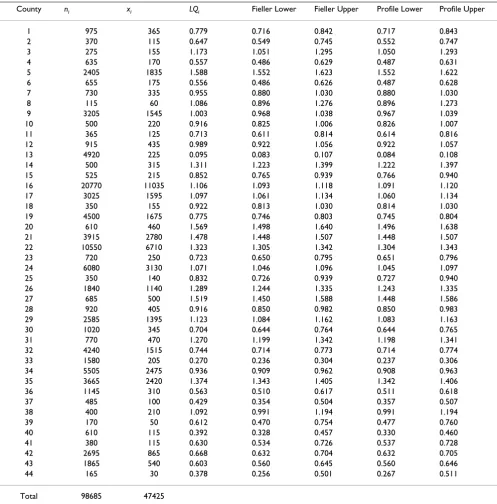
Application to health utilization data

In this section, the different methods of estimating confi-dence interval for the location quotient are illustrated using a health utilization data set from Ontario, Canada. Data were extracted from the Ontario Health Insurance Plan (OHIP) database for all ambulatory specialist visits due to rheumatoid arthritis in the fiscal year 1996. The vis-its were assigned to census divisions based on where the patient was registered and not where services were received. Forty four censuses divisions were used for anal-ysis. For each county, the LQ is defined as the ratio of two proportions with the numerator representing the number of visits to rheumatologists in the census division divided by the total number of specialist visits in the census divi-sion, and the denominator defined as the number of visits to rheumatologists for the province divided by the total number of specialist visits in the province.

For a given county, a location quotient of less than one indicates that the utilization of health care services is under represented compared to the provincial utilization rate. On the other hand, a location quotient of greater than one suggests that health care services utilization is greater than expected. A location quotient of one indicates lack of under or over concentration of utilization in the census division.

Table 2 shows the data, along with the estimated location quotients and confidence intervals. The intervals based on the delta and Fieller's methods were identical to three dec-imal places. Therefore only the Fieller's lower and upper limits are shown in Table 2 and compared with the inter-vals based on the profile-likelihood results in the general-ized linear models.

There is a remarkable agreement in the confidence inter-vals from both the Fieller and profile-likelihood approaches due to the fact that the denominator of the ratio is estimated with sufficiently high precision, which would be the case for applications with large sample sizes. Small relative differences are observed when sample sizes are small, as in counties 39 and 44 in Table 2.

The LQ was significantly greater than 1, which is the entire confidence interval falls above 1, for 32% (14/44) of the census divisions, indicating significantly higher utiliza-tion of health care services for rheumatoid arthritis than

the provincial rate. Similarly, 52% (23/44) of the census divisions showed a significantly lower utilization rate. The remaining 16% experienced a utilization rate compatible with the provincial rate.

Discussion

The location quotient (LQ) is one of several spatial meas-ures that is widely used to examine spatial variation of area characteristics [14]. However, a frequently occurring 'gap' is the widespread use of LQ as a point estimate with-out an accompanying confidence interval. In this paper, we have demonstrated that confidence intervals for ratio Table 2: Location quotients for health utilization data, with 95% lower and upper confidence limits using (1) Fieller's and (2) Profile-likelihood methods (see text for details about the data and methods)

County ni xi LQi Fieller Lower Fieller Upper Profile Lower Profile Upper

1 975 365 0.779 0.716 0.842 0.717 0.843

2 370 115 0.647 0.549 0.745 0.552 0.747

3 275 155 1.173 1.051 1.295 1.050 1.293

4 635 170 0.557 0.486 0.629 0.487 0.631

5 2405 1835 1.588 1.552 1.623 1.552 1.622

6 655 175 0.556 0.486 0.626 0.487 0.628

7 730 335 0.955 0.880 1.030 0.880 1.030

8 115 60 1.086 0.896 1.276 0.896 1.273

9 3205 1545 1.003 0.968 1.038 0.967 1.039

10 500 220 0.916 0.825 1.006 0.826 1.007

11 365 125 0.713 0.611 0.814 0.614 0.816

12 915 435 0.989 0.922 1.056 0.922 1.057

13 4920 225 0.095 0.083 0.107 0.084 0.108

14 500 315 1.311 1.223 1.399 1.222 1.397

15 525 215 0.852 0.765 0.939 0.766 0.940

16 20770 11035 1.106 1.093 1.118 1.091 1.120

17 3025 1595 1.097 1.061 1.134 1.060 1.134

18 350 155 0.922 0.813 1.030 0.814 1.030

19 4500 1675 0.775 0.746 0.803 0.745 0.804

20 610 460 1.569 1.498 1.640 1.496 1.638

21 3915 2780 1.478 1.448 1.507 1.448 1.507

22 10550 6710 1.323 1.305 1.342 1.304 1.343

23 720 250 0.723 0.650 0.795 0.651 0.796

24 6080 3130 1.071 1.046 1.096 1.045 1.097

25 350 140 0.832 0.726 0.939 0.727 0.940

26 1840 1140 1.289 1.244 1.335 1.243 1.335

27 685 500 1.519 1.450 1.588 1.448 1.586

28 920 405 0.916 0.850 0.982 0.850 0.983

29 2585 1395 1.123 1.084 1.162 1.083 1.163

30 1020 345 0.704 0.644 0.764 0.644 0.765

31 770 470 1.270 1.199 1.342 1.198 1.341

32 4240 1515 0.744 0.714 0.773 0.714 0.774

33 1580 205 0.270 0.236 0.304 0.237 0.306

34 5505 2475 0.936 0.909 0.962 0.908 0.963

35 3665 2420 1.374 1.343 1.405 1.342 1.406

36 1145 310 0.563 0.510 0.617 0.511 0.618

37 485 100 0.429 0.354 0.504 0.357 0.507

38 400 210 1.092 0.991 1.194 0.991 1.194

39 170 50 0.612 0.470 0.754 0.477 0.760

40 610 115 0.392 0.328 0.457 0.330 0.460

41 380 115 0.630 0.534 0.726 0.537 0.728

42 2695 865 0.668 0.632 0.704 0.632 0.705

43 1865 540 0.603 0.560 0.645 0.560 0.646

44 165 30 0.378 0.256 0.501 0.267 0.511

Publish with BioMed Central and every scientist can read your work free of charge "BioMed Central will be the most significant development for disseminating the results of biomedical researc h in our lifetime."

Sir Paul Nurse, Cancer Research UK

Your research papers will be:

available free of charge to the entire biomedical community

peer reviewed and published immediately upon acceptance

cited in PubMed and archived on PubMed Central

yours — you keep the copyright

Submit your manuscript here:

http://www.biomedcentral.com/info/publishing_adv.asp

BioMedcentral

parameters in general and location quotients in particular can be obtained using a number of complimentary approaches. Three techniques – the delta method, Fieller's interval, and profile-likelihood based interval from a gen-eralized linear model – are presented and illustrated. We also demonstrated that if the denominator of the ratio is estimated with sufficiently high precision, then the meth-ods introduced in this paper will produce very similar confidence intervals. The normal approximation to the binomial is used for the variance estimate for the calcula-tion by the delta and Fieller methods. Hence it is not sur-prising that these methods do not perform well for small sample sizes and extreme proportions.

The techniques we described are generic and can be applied to a wide range of settings where ratio parameters are in use. The generalized linear model (GLM) approach is particularly appealing since the parameters of interest (in our application the location quotients) are estimated directly along with confidence intervals and significance levels. These considerations can be important in practical applications where there are several parameters to be esti-mated. For instance, for the health utilization data set we analyzed in this paper, 44 location quotients and their confidence intervals had to be generated and the model-ling approach was the preferred method over the delta and Fieller's techniques.

Competing interests

The author(s) declare that they have no competing interests.

Authors' contributions

JB initiated, designed, and drafted the study. Both JB and RM participated in simulating, analyzing, and discussing the results and in writing the paper. All authors read and approved the final manuscript.

Acknowledgements

The authors would like to acknowledge helpful comments by the reviewers. JB acknowledges the support of the Research Institute at the Hospital for Sick Children.

References

1. Thrall GI, Borden E, Thrall S: Delineating Hospital Trade Areas.

GeoSpatial Solution 2002, 12:46-51.

2. Cortese CF, Leftwich JE: A technique for measuring the effect of economic base on opportunity for blacks. Demography 1975, 12:325-329.

3. Robinson GM: Methods and Techniques in Human Geography Toronto: John Wiley & Sons; 1998.

4. Fleiss JL: Statistical Methods for Rates and Proportions New York: John Wiley & Sons; 1981.

5. Moineddin R, Beyene J, Boyle E: On the location quotient confi-dence interval. Geographical Analysis 2003, 35:249-256.

6. Oehlert GW: A note on the delta method. American Statistician

1992, 46:27-29.

7. Fieller EC: The biological standardization of Insulin. Suppl to J R Statist Soc 1940, 7:1-64.

8. Cordell HJ, Elston RC: Fieller's theorem and linkage disequilib-rium mapping. Genet Epidemiol 1999, 17:237-252.

9. Polsky D, Glick HA, Willke R, Schulman K: Confidence intervals for cost-effectiveness ratios: a comparison of four methods.

Health Econ 1997, 6:243-252.

10. Silcocks P: Estimating confidence limits on a standardized mortality ratio when the expected number is not error free.

J Epidemiol Community Health 1994, 48:313-317.

11. McCullagh P, Nelder JA: Generalized Linear Models 2nd edition. New York: Chapman and Hall; 1989.

12. SAS Institute Inc: SAS/STAT User's Guide, Version 8 SAS Institute, Cary, NC; 1999.

13. Knight K: Mathematical statistics New York: Chapman and Hall/CRC Press; 2000.

14. Thrall GI, Fandrich J, Elshaw-Thrall S: Location quotient: Descrip-tive geography for the community reinvestment act. Geo Info Systems 1995, 5:18-22.

Pre-publication history

The pre-publication history for this paper can be accessed here: