Open Access
Research article
How does correlation structure differ between real and fabricated
data-sets?
Noori Akhtar-Danesh*
1and Mahshid Dehghan-Kooshkghazi
2Address: 1School of Nursing & Department of Clinical Epidemiology and Biostatistics, McMaster University, Hamilton, Canada and 2Population
Health Research Institute, Department of Medicine, McMaster University, Hamilton, Canada
Email: Noori Akhtar-Danesh* - [email protected]; Mahshid Dehghan-Kooshkghazi - [email protected] * Corresponding author
Abstract
Background: Misconduct in medical research has been the subject of many papers in recent years. Among different types of misconduct, data fabrication might be considered as one of the most severe cases. There have been some arguments that correlation coefficients in fabricated data-sets are usually greater than that found in real data-sets. We aim to study the differences between real and fabricated data-sets in term of the association between two variables.
Method: Three examples are presented where outcomes from made up (fabricated) data-sets are compared with the results from three real data-sets and with appropriate simulated data-sets. Data-sets were made up by faculty members in three universities. The first two examples are devoted to the correlation structures between continuous variables in two different settings: first, when there is high correlation coefficient between variables, second, when the variables are not correlated. In the third example the differences between real data-set and fabricated data-sets are studied using the independent t-test for comparison between two means.
Results: In general, higher correlation coefficients are seen in made up data-sets compared to the real data-sets. This occurs even when the participants are aware that the correlation coefficient for the corresponding real data-set is zero. The findings from the third example, a comparison between means in two groups, shows that many people tend to make up data with less or no differences between groups even when they know how and to what extent the groups are different.
Conclusion: This study indicates that high correlation coefficients can be considered as a leading sign of data fabrication; as more than 40% of the participants generated variables with correlation coefficients greater than 0.70. However, when inspecting for the differences between means in different groups, the same rule may not be applicable as we observed smaller differences between groups in made up compared to the real data-set. We also showed that inspecting the scatter-plot of two variables can be considered as a useful tool for uncovering fabricated data.
Background
Misconduct in medical research has been the subject of many papers in recent years [1–5]. The usual types of mis-conduct include fabrication and falsification of data,
pla-giarism, deceptive reporting of results, suppression of existing data, and deceptive design or analysis [4,6]. At the same time, there has been much effort to reveal fraudulent data and to equip statisticians with some techniques for
Published: 29 September 2003
BMC Medical Research Methodology 2003, 3:18
Received: 26 June 2003 Accepted: 29 September 2003
This article is available from: http://www.biomedcentral.com/1471-2288/3/18
detecting such data [7,8]. In a recent paper, the roles of biostatisticians in preventing and detecting of fraud in clinical trials have been discussed and different methods for detecting fraudulent data have been suggested [6]. For instance, it has been shown in many articles that the standard deviation for fabricated data is less than that of the corresponding real data [8] and there are arguments that the correlation coefficient between two variables in a fabricated data-set is usually greater than that of the real data-set [6]. However, we could not find any paper about the correlation structure of fabricated data in the literature.
In this article we study an extreme case of fraud, i.e. data fabrication, which could have much more effect on con-clusions drawn from medical research than any other type of fraud. Particularly, we emphasise on some simple tech-niques that might be useful for detecting fabricated data. The techniques are based on the relationship between var-iables. These methods could be useful not just because of the ethics that must be observed in the research process but because of the possible consequences that fabricated data could have on health care practice.
Methods
In this work three examples of real data-sets are consid-ered. For the first two data-sets our main objective is to find out how closely the correlation structures of real data-sets could be reconstructed with fabricated data. In order to investigate the correlation structure of fabricated data, summary statistics of two real data-sets were shown to the faculty members at Shiraz Medical School and Jahrom Medical School in Iran. These faculty members were from the departments of clinical and basic sciences including Community Medicine, Microbiology, Physiology, Paedi-atrics, Internal Medicine, etc. Statisticians and epidemiol-ogists were not asked to participate in this study. We met each faculty member in person and spent about 10 to 30 minutes to explain our objectives and the summary statis-tics of the two real data-sets. Then, they were asked to make up similar data-sets for 40 hypothetical subjects using forms provided as if they were attempting fraud by fabricating data for a real study.
The sample size of 40 hypothetical subjects is based on the following considerations. To detect a correlation coef-ficient greater than 0.40 with type 1 error 0.05 and power 0.80 a sample size of 37 is sufficient (9). We felt that our colleagues would be willing to make up as many as 40 data-points, so there would be good power to detect cor-relation of 0.40. The results proved that this sample size was enough for most cases.
Respondents were asked to make up their data within the same range indicated by the real data-sets. Thirty-four
people returned their completed forms within one week, providing 34 data-sets for each example which are ana-lysed in this article.
In Example 3 the mean of a continuous variable is com-pared between two groups. This does not deal directly with the correlation coefficient between two continuous variables, but provides a further instance of how made up data-sets can be differentiated from the corresponding real data-set. This can be regarded as an example of asso-ciation between a continuous and a categorical variable. Each respondent was asked to make up data for 30 hypo-thetical subjects in each group. Based on the observed means and standard deviations of the real data-set, type 1 error of 0.05, and power of 0.80, a sample size of 25 in each group is sufficient. To be more conservative we chose sample size 30 in each group.
In all examples the made up data-sets were produced "by hand".
For each example the results from the made up data-sets are compared with results of 2500 appropriate computer-generated data-sets. These simulated random samples are drawn with replacement either based on the specifications of the corresponding real data-set and the theory of nor-mal distribution (Example 1 and Example 3) or from the real data-set (Example 2).
Results
In this section the differences between the real and made up data-sets are shown in term of the association between variables.
Example 1
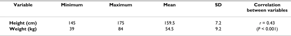
In this example we consider two variables which are highly correlated. Table 1 shows some descriptive statis-tics of the height and weight of 65 female students aged 20–22 studying at Jahrom Medical School, autumn 2001. The correlation between the two variables is highly
signif-icant (r = 0.43, P < 0.001). We gave this table to the
par-ticipants and asked them to make up measurements of height and weight for 40 hypothetical female students as if they were fabricating data for a real study.
Correlation coefficients of the 34 made up data-sets ranged from -0.097 to 0.996 (mean = 0.33, SD = 0.33). Figure 1 shows the scatter-plots of these data-sets. Most participants produced data-sets with correlation coeffi-cients greater than that of the real data-set.
standard deviations of height and weight observed in the real data-set (see Table 1) and the theory of the bivariate normal distribution. For each simulated data-set correla-tion between height and weight was tested against the null
hypothesis of ρ = 0.43 and the corresponding p-value was
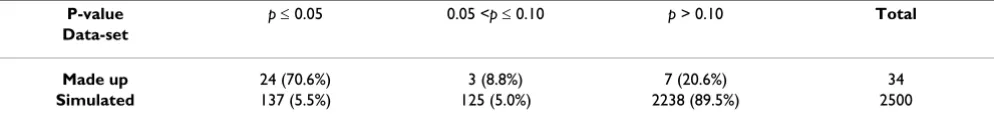
recorded. A comparison between the correlation coeffi-cients of these simulated sets and the made up data-sets are shown in Table 2. Using a Fisher's exact test indi-cates that the correlation structures are different between made up data-sets and the simulated data-sets (P <0.0001).
In addition, 19 (56%) of these made up data-sets had cor-relation coefficients greater than 0.43. The corcor-relation coefficient in 18 (53%) data-sets was greater than 0.70, and in ten (29%) was 0.90 or higher. In comparison, only 5.5% of the simulated data-sets had correlation coeffi-cients statistically different from 0.43. Thus, the made up (fabricated) data-sets yielded considerably higher correla-tion coefficients than the corresponding real or randomly generated data-sets.
Example 2
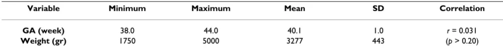
In this example two variables are considered which are not expected to be correlated or at least very modestly cor-related. Figure 2 shows the scatter-plot of birth weight by gestational age (GA) in 637 newborn boys. Gestational age ranges from 38 to 44 weeks. These data were collected from the birth records of four hospitals in Shiraz, Iran [10]. It can be easily concluded from Figure 2 that these
variables are not correlated (r = 0.031, p = 0.437). Table 3
presents the summary statistics of gestational age and birth weight for these babies.
Table 3 was provided to the participants and they were asked to make up gestational age and birth weight for 40 hypothetical babies in the same range as shown by Table 3, as if they were fabricating the data instead of collecting the real data.
The correlation coefficients between gestational age and birth weight for the 34 made up data-sets were in the range -0.36 to 0.98. Of these data-sets 22 (65%) were sig-nificantly different from zero (see also Figure 3). A simu-lation study was carried out to determine whether these
made up sets resemble samples from the real data-set. We drew 2500 random samples of size 40 from the real data-set of which only 109 (4.4%) data-sets had cor-relation coefficients different from zero. A comparison between the results of the made up data-sets and 2500 random samples from the real data-set is given in Table 4. Fisher's exact test, indicates that correlations in fabricated data-sets are different than those in random samples from
the real data-set (P <0.0001).
Furthermore, in the 22 made up data-sets with correlation coefficients statistically different from zero, 20 (59%) of them had a positive correlation coefficient and only in two the correlation coefficient was negative. Indeed, in 13 (38%) of them the correlation coefficient was greater than 0.70 and in 5 (15%) more than 0.90.
Example 3
In a study conducted at McMaster University in Canada, 45 graduating students of nursing from a problem based learning (PBL) curriculum were compared with 31 stu-dents from a more conventional curriculum at the Univer-sity of Ottawa [11]. One variable on which they were compared was the students' perceived ability to
commu-nicate with patients or so-called communication skill. The
summary statistics of the communication skill for both groups are provided in Table 5.
This table was sent by e-mail to the all faculty members at the School of Nursing at McMaster University and they were asked to generate data-sets for 30 hypothetical stu-dents in each group based on the information of the table, as if they were making up data instead of assessing it from real subjects. Seventeen faculty members responded before the specified deadline. For these 17 data-sets the mean difference between groups ranged from -0.057 to 4.63. Only 9 (53%) of these differences were significantly different from zero. Figure 4 represents the box-plots for these made up data-sets along with the box-plot of the real data-set.
As Figure 4 shows, compared to the real data-set many participants produced data-sets with smaller mean differ-ences between groups which was surprising as we were expecting larger differences between groups. It could have
Table 1: Summary statistics of height and weight for 65 students
Variable Minimum Maximum Mean SD Correlation between variables
Height (cm) 145 175 159.5 7.2 r = 0.43
Scatter-plot of weight and height for data-sets made up by 34 individuals
Figure 1
Scatter-plot of weight and height for data-sets made up by 34 individuals
Weight
140 150 160 170 180 190
40
60
80
140 150 160 170 180 190
40
60
80
140 150 160 170 180 190
40
60
80
140 150 160 170 180 190
40
60
80
140 150 160 170 180 190
40
60
80
Weight
140 150 160 170 180 190
40
60
80
140 150 160 170 180 190
40
60
80
140 150 160 170 180 190
40
60
80
140 150 160 170 180 190
40
60
80
140 150 160 170 180 190
40
60
80
Weight
140 150 160 170 180 190
40
60
80
140 150 160 170 180 190
40
60
80
140 150 160 170 180 190
40
60
80
140 150 160 170 180 190
40
60
80
140 150 160 170 180 190
40
60
80
Weight
140 150 160 170 180 190
40
60
80
140 150 160 170 180 190
40
60
80
140 150 160 170 180 190
40
60
80
140 150 160 170 180 190
40
60
80
140 150 160 170 180 190
40
60
80
Weight
140 150 160 170 180 190
40
60
80
140 150 160 170 180 190
40
60
80
140 150 160 170 180 190
40
60
80
140 150 160 170 180 190
40
60
80
140 150 160 170 180 190
40
60
80
Weight
140 150 160 170 180 190
40
60
80
140 150 160 170 180 190
40
60
80
140 150 160 170 180 190
40
60
80
140 150 160 170 180 190
40
60
80
Height 140 150 160 170 180 190
40
60
80
Height
Weight
140 150 160 170 180 190
40
60
80
Height 140 150 160 170 180 190
40
60
80
Height 140 150 160 170 180 190
40
60
80
Height 140 150 160 170 180 190
40
60
happened by chance as the number of respondents was
small (n = 17). On the other hand, it might be the nature
of the fabricated data for comparing two treatment groups. In other words, observing large differences
between groups for fabricated data might not be a reason-able and justified expectation. All in all, those are the only made up data-sets of this type that we are aware of and
Table 2: Comparison between the significance levels of the correlations for the made up data-sets and 2500 random samples produced based on the specifications of Table 1*
P-value p ≤ 0.05 0.05 <p ≤ 0.10 p > 0.10 Total Data-set
Made up 24 (70.6%) 3 (8.8%) 7 (20.6%) 34
Simulated 137 (5.5%) 125 (5.0%) 2238 (89.5%) 2500
* data-sets with p-value ≤ 0.05 were compared with p-value > 0.05, (Fisher's exact test, p < 0.0001)
Scatter-plot of birth weight by gestational age for 637 newborn boys
Figure 2
Scatter-plot of birth weight by gestational age for 637 newborn boys
37
38
39
40
41
42
43
44
Gestational age
2000
3000
4000
5000
Birth
Table 3: Summary statistics of gestational age (GA) and birth weight for 637 newborn boys
Variable Minimum Maximum Mean SD Correlation
GA (week) 38.0 44.0 40.1 1.0 r = 0.031
Weight (gr) 1750 5000 3277 443 (p > 0.20)
Scatter-plot of birth weight and gestational age for 34 made up data-sets
Figure 3
Scatter-plot of birth weight and gestational age for 34 made up data-sets
Birth w
eight
36 38 40 42 44
2000
4000
36 38 40 42 44
2000
4000
36 38 40 42 44
2000
4000
36 38 40 42 44
2000
4000
36 38 40 42 44
2000
4000
Birth w
eight
36 38 40 42 44
2000
4000
36 38 40 42 44
2000
4000
36 38 40 42 44
2000
4000
36 38 40 42 44
2000
4000
36 38 40 42 44
2000
4000
Birth w
eight
36 38 40 42 44
2000
4000
36 38 40 42 44
2000
4000
36 38 40 42 44
2000
4000
36 38 40 42 44
2000
4000
36 38 40 42 44
2000
4000
Birth w
eight
36 38 40 42 44
2000
4000
36 38 40 42 44
2000
4000
36 38 40 42 44
2000
4000
36 38 40 42 44
2000
4000
36 38 40 42 44
2000
4000
Birth w
eight
36 38 40 42 44
2000
4000
36 38 40 42 44
2000
4000
36 38 40 42 44
2000
4000
36 38 40 42 44
2000
4000
36 38 40 42 44
2000
4000
Birth w
eight
36 38 40 42 44
2000
4000
36 38 40 42 44
2000
4000
36 38 40 42 44
2000
4000
36 38 40 42 44
2000
4000
Gestational age 36 38 40 42 44
2000
4000
Gestational age
Birth w
eight
36 38 40 42 44
2000
4000
Gestational age 36 38 40 42 44
2000
4000
Gestational age 36 38 40 42 44
2000
4000
Gestational age 36 38 40 42 44
2000
Table 4: Comparison between the made up data-sets and 2500 real random samples from 637 newborn boys of the p-values of the correlation between GA and birth weight+
P-value p ≤ 0.05 0.05 <p ≤ 0.10 p > 0.10 Total Data-set
Fabricated 22 (64.7%) 1 (2.9%) 11 (32.4%) 34
Samples from the Real data-set 109 (4.4%) 113 (4.5%) 2278 (91.1%) 2500
+ data-sets with p-value ≤ 0.05 were compared with p-value > 0.05, (Fisher's exact test, p < 0.0001)
Table 5: Summary statistics of communication skill in two groups of students
Group (No.) Minimum Maximum Mean SD Comparison
PBL (45) 12 24 19.1 2.8 t = 3.66
Conventional (31) 8 22 16.6 3.4 p < 0.001
Box-plots of 17 made up and the real data-sets for the two different curriculum
Figure 4
Box-plots of 17 made up and the real data-sets for the two different curriculum
much more needs to be done to find out the true nature of fabricated data for comparing means between groups.
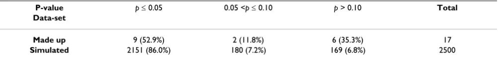
Again, 2500 data-sets were generated based on the specifi-cations of Table 5 and the theory of normal distribution. An independent t-test was used to compare the means between two groups in each data-set. Fisher's exact test indicates that the data structures between made up and simulated data-sets are different (Table 6, P = 0.0011).
Discussion
In this research we aimed to find out similarities and dif-ferences between real and made up data-sets regarding the association between variables. Although the made up data-sets for this research are not real cases of fabricated data, participants were asked to make up data as close as possible to real data, an inclination which is prominent in data fabrication.
In the first two examples we focused on the Pearson cor-relation coefficient. The third example is not directly about correlation between variables. However, it relates to the association between a categorical variable, dichoto-mous here, and a continuous variable.
About 30 percent of participants in Example 1 produced data with correlation coefficients greater than 0.90 between height and weight, where the correlation coeffi-cient for the real data-set was 0.43. In Example 2, 15 per-cent of participants produced data with correlation coefficient greater than 0.90 even though there was no correlation between birth weight and gestational age
(ges-tational age ≥ 38 weeks). Except in longitudinal data
where large correlation coefficients occur when the same variable is observed at close time-points, correlation coef-ficients above 0.80 are not often seen. Therefore, a high correlation coefficient could be regarded as a key point for suspicion when checking for fabricated data.
In Example 3, the expectation was that participants would produce data with larger mean differences between groups than in the corresponding real data, but they produced data with smaller differences. This could be because of the
small number of respondents (n = 17). On the other
hand, the expectation of observing greater differences between groups, consistent with what we observed for correlations between continuous variables, might not be applicable here. To our knowledge, little, if any, has been done on detecting fabricated data by comparing mean val-ues between groups. This article may be considered as the first step in this regard and much more is needed to be done.
As the last point, there was a considerable number of non-respondents in this survey. Although we never can expect to obtain 100 percent response rate, there were some other factors which could have affected this study. First, some people may hesitate to make up data even when they know that it is used just for research purposes. Sec-ond, our request for making up data-sets for Example 3 was circulated to the faculty members at the School of Nursing at the end of the winter semester. At that time fac-ulty members were busy with exams and marking, so would have had little time to participate in the study.
Conclusion
In this survey made up data-sets were used to find out the similarities and differences between fabricated and real data-sets. The results indicate that high correlation coefficients can be considered as a potential sign of data fabrication. However, for differences between mean val-ues in different groups, the same rule may not apply. We also showed that inspecting a scatter-plot of two variables can be a useful tool for uncovering fabricated data. As Bai-ley [8] concluded, statistical inference is necessary but may not be sufficient for detecting fabricated data. Some-times inspecting appropriate graphs could be much more informative than applying statistical techniques and tests.
Authors' contributions
NAD was mainly responsible for analysis and MDK for collecting data and data entry. Both contributed equally in designing the study and drafting the manuscript.
Acknowledgments
We are grateful to Dr Elizabeth Rideout for making available to us the data-set for Example 3. We also benefited from her invaluable comments on the first draft of this article. We are thankful to Professor Harry Shannon for his comments and reading the final draft. We are also thankful to the
refe-Table 6: Comparison between made up and simulated data-sets about communication skill++
P-value p ≤ 0.05 0.05 <p ≤ 0.10 p > 0.10 Total Data-set
Made up 9 (52.9%) 2 (11.8%) 6 (35.3%) 17
Simulated 2151 (86.0%) 180 (7.2%) 169 (6.8%) 2500
Publish with BioMed Central and every scientist can read your work free of charge
"BioMed Central will be the most significant development for disseminating the results of biomedical researc h in our lifetime."
Sir Paul Nurse, Cancer Research UK
Your research papers will be:
available free of charge to the entire biomedical community
peer reviewed and published immediately upon acceptance
cited in PubMed and archived on PubMed Central
yours — you keep the copyright
Submit your manuscript here:
http://www.biomedcentral.com/info/publishing_adv.asp
BioMedcentral
rees for their invaluable comments. We would like to thank our colleagues at Jahrom Medical School, Shiraz University of Medical Sciences, and School of Nursing at McMaster University for making up the data-sets. Our stu-dents at Jahrom Medical School kindly provided us their height and weight measurements for Example 1.
References
1. Horton R: The clinical trial: Deceitful, disputable, unbelieva-ble, unhelpful, and shameful – What next?Controlled Clinical Trials 2001, 22:593-604.
2. Neaton JD, Bartsch GE, Broste SD, Cohen JD and Simon NM: A case of data alteration in the multiple risk factor intervention trial (MRFIT). Controlled Clinical Trials 1991, 12:731-740.
3. Ranstam J, Buyse M and George SL et al.: Fraud in medical research: an international survey of biostatisticians. Controlled Clinical Trials 2000, 21:415-427.
4. Riis P: Scientific dishonesty: European reflections. Journal of Clinical Pathology 2001, 54:4-6.
5. White C: Plans for tackling research fraud may not go far enough. British Medical Journal 2000, 321:1487.
6. Buyse M, George SL and Evans S et al.: The role of biostatistics in the prevention, detection and treatment of fraud in clinical trials. Statistics in Medicine 1999, 18:3435-3451.
7. DeMets DL: Distinctions between fraud, bias, errors, misun-derstanding, and incompetence.Controlled Clinical Trials 1997,
18:637-650.
8. Bailey KR: Detecting fabrication of data in a multicenter col-laborative animal study. Controlled Clinical Trials 1991, 12:741-752. 9. Machin D, Campbell M, Fayers P and Pinol A: Sample Size Tables for
Clinical Studies Oxford: Blackwell Science; 1997.
10. Akhtar-Danesh N: The incidence of congenital malformation in Southern Iran, 1987–1988: an epidemiological survey. MSc thesis Shiraz University of Medical Sciences; 1988.
11. Rideout E, England-Oxford V and Brown B et al.: A comparison of problem-based and conventional curricula in nursing education. Advances in Health Sciences Education 2002, 7:3-17.
Pre-publication history
The pre-publication history for this paper can be accessed here: