Sensitivity Analysis of Synchronous Generators for Real-Time Simulation

(1)

University of New Orleans University of New Orleans

ScholarWorks@UNO

University of New Orleans Theses and

Dissertations Dissertations and Theses

Spring 5-13-2016

Sensitivity Analysis of Synchronous Generators for Real-Time

Simulation

Sowmya Munukuntla

University of New Orleans, [email protected]

Follow this and additional works at: https://scholarworks.uno.edu/td

Part of the Electrical and Electronics Commons, and the Power and Energy Commons

Recommended Citation Recommended Citation

Munukuntla, Sowmya, "Sensitivity Analysis of Synchronous Generators for Real-Time Simulation" (2016). University of New Orleans Theses and Dissertations. 2172.

https://scholarworks.uno.edu/td/2172

This Thesis is protected by copyright and/or related rights. It has been brought to you by ScholarWorks@UNO with permission from the rights-holder(s). You are free to use this Thesis in any way that is permitted by the copyright and related rights legislation that applies to your use. For other uses you need to obtain permission from the rights-holder(s) directly, unless additional rights are indicated by a Creative Commons license in the record and/or on the work itself.

(2)

Sensitivity Analysis of Synchronous Generators for Real-Time

Simulation

A Thesis

Submitted to the Graduate Faculty of the

University of New Orleans

in partial fulfillment of the

requirements of the degree of

Master of Science

in

Engineering

Electrical Engineering

By

Sowmya Munukuntla

B-Tech. Jawaharlal Nehru Technological University, 2012

(3)

Acknowledgement

Firstly, I would like to thank my parents and brother for their encouragement and unconditional support in every aspect of my life. Without their support, this would not be possible.

I sincerely acknowledge the support and encouragement received from my research and academic adviser Dr. Parviz Rastgoufard for his continuous

support through out my graduate study and research. His patience and

unfailing encouragement have been the major contributing factors in the completion of my thesis research.

I heartfully thank Dr. Ittiphong Leevongwat for his valuable suggestions and technical support throughout my thesis and research work. He was available in all the tough times and strongly supported and corrected the work throughout my academics.

I sincerely thank Dr. Ebrahim Amiri for his continuous moral support

throughout my study at the school. I thank him for keeping me motivated and boost up the confidence during my research.

I further sincerely appreciate and thank my friends Rastin Rastgoufard and Ram Mohan Snaboyina for their time and help in achieving the software knowledge. I also thank UNO-Entergy Power and Energy Research Laboratory (PERL) for giving me access to all the software needed.

Finally, I would like to thank all the faculty and staff members of the College of Engineering at University of New Orleans for their support and contribution in providing quality education.

(4)

List of Figures

2.1 Round Rotor Generator(GENROU) Model Block Diagram [3] . . . 13

2.2 Equivalent circuit of two-winding transformer . . . 17

2.3 Per unit equivalent circuit . . . 20

2.4 Equivalentπ transmission line . . . 22

3.1 Flow chart for performing Steady State Analysis . . . 27

3.2 Flow chart for performing Dynamic Analysis . . . 28

3.3 IEEE Type-1 Exciter Block Diagram [9] . . . 32

3.4 Transfer function block diagram with three step inputs . . . 36

3.5 Output of the transfer function block diagram with three step inputs . . . . 37

3.6 Overall transfer function with a step input . . . 37

3.7 Output of the overall transfer function with a step input . . . 38

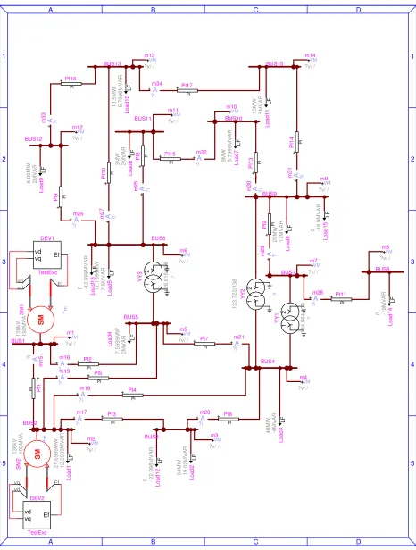
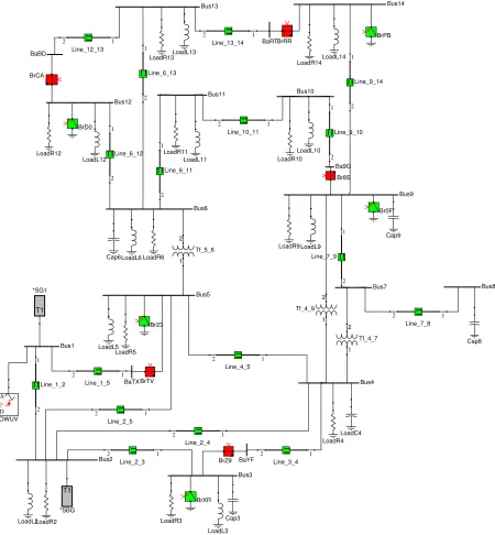
3.8 Variation of TF; Voltage at Bus 1, Bus 2, Bus 3 (in pu) with respect to time 42 3.9 Variation of KF; Voltage at Bus 1, Bus 2, Bus 3 (in pu) with respect to time 42 3.10 Variation of KA; Voltage at Bus 1, Bus 2, Bus 3 (in pu) with respect to time 43 3.11 Variation of TE; Voltage at Bus 1, Bus 2, Bus 3 (in pu) with respect to time 43 3.12 Variation of KE; Voltage at Bus 1, Bus 2, Bus 3 (in pu) with respect to time 43 3.13 Variation of TA; Voltage at Bus 1, Bus 2, Bus 3 (in pu) with respect to time 43 3.14 Variation of TR; Voltage at Bus 1, Bus 2, Bus 3 (in pu) with respect to time 44 4.1 IEEE 14 Bus Test System [8] . . . 48

5.1 IEEE 14 Bus Test System in PSS/E . . . 55

5.2 IEEE 14 Bus Test System in EMTP . . . 56

5.3 IEEE 14 Bus Test System in Hypersim . . . 57

5.4 IEEE Type-1 Exciter modeled in EMTP . . . 58

5.5 IEEE Type-1 Exciter modeled in Hypersim . . . 58

5.6 Overlapped voltages (in pu) at Bus-1, Bus-2, Bus-5 from PSS/E, EMTP and Hypersim for fault at Bus-5. . . 62

5.7 Overlapped voltages (in pu) at Bus-1, Bus-2, Bus-5 from PSS/E, EMTP, and Hypersim with variation of KF and TF in PSS/E for fault at Bus-5. . . 65

5.8 Overlapped voltages (in pu) at Bus-1, Bus-2, Bus-5 from PSS/E, EMTP, and Hypersim with variation of TE in PSS/E for fault at Bus-5. . . 66

5.9 Overlapped voltages (in pu) at Bus-1, Bus-2, Bus-5 from PSS/E, EMTP, and Hypersim with variation of KE in PSS/E for fault at Bus-5. . . 67

5.10 Overlapped voltages (in pu) at Bus-1, Bus-2, Bus-5 from PSS/E, EMTP, and Hypersim with variation of KA in PSS/E for fault at Bus-5. . . 68

5.11 Overlapped voltages (in pu) at Bus-1, Bus-2, Bus-5 from PSS/E, EMTP and Hypersim for fault at Bus-5. . . 69

(7)

5.13 Overlapped voltages (in pu) at Bus-1, Bus-2, Bus-6 from PSS/E, EMTP and

Hypersim for fault at Bus-6 with removal of shunt capacitor. . . 72

1 Overlapped voltages (in pu) at Bus-1, Bus-2, Bus-3 from PSS/E, EMTP and

Hypersim for fault at Bus-3. . . 80

(8)

List of Tables

3.1 Parameter values for calculating sensitivity . . . 41

3.2 Parameter’s range for the sensitivity analysis . . . 41

3.3 Parameter Ranking based on Sensitivity . . . 42

4.1 Bus Data . . . 49

4.2 Transmission Line Parameters . . . 50

4.3 Transformer Parameters . . . 50

4.4 Load Parameters . . . 51

4.5 Generator Parameters . . . 51

4.6 Generator (GENROU) Dynamic Parameters . . . 52

4.7 Exciter (IEEET1) Parameters . . . 53

5.1 Voltages (kV RMS) compared between PSSE, EMTP, and Hypersim . . . . 60

5.2 Currents (A RMS) compared between PSSE, EMTP, and Hypersim . . . 60

(9)

Abstract

The purpose of this thesis is to validate generator models for dynamic studies of

power systems using PSS/E (Power System Simulator for Engineering), EMTP

(ElectroMagnetic Transient Program), and Hypersim. To thoroughly evaluate

the behavior of a power system in the three specified software packages, it

is necessary to have an accurate model for the power system, especially the

generator which is of interest. The effect of generator modeling on system

response under normal conditions and under faulted conditions is investigated

in this work. A methodology based on sensitivity analysis of generator model

parameters is proposed aiming to homogenize the behavior of the same power

system that is modeled in three software packages. Standard IEEE 14-Bus

system is used as a test case for this investigation. Necessary changes in the

exciter parameters are made using the proposed methodology so that the

system behaves identical across all three software platforms.

Keywords: PSS/E, EMTP, Hypersim, Real-Time Modeling, Generator Modeling, Exciter Modeling, Exciter Parameters, Sensitivity Analysis, IEEE

(10)

Chapter 1 Problem Statement and Historical

Review

1.1 Introduction

In a power system network consisting of generation, transmission and distribution, synchronous

generators are the major power generating units where as motors are the major loads which

makes the synchronous machine an important element in the power system. In order to have

a more reliable power system and quick response for the faults in the system, more accurate

modeling of the synchronous machine is necessary.

Two groups of investigators developed ways to accurately model a synchronous generator

starting from later part of twentieth century during which there was an increased interest

in modeling of synchronous machines. One group among the two tried to compare the

performance of the synchronous machine models with the measured performance of the

machines with a fault applied on the system. The other group developed an alternate method

of finding the machine parameters which can be used in the models so that the performance

matches the actual measurements.

There are quite different kinds of power system software used by the Engineers but every

software platform has their own limitations. Few software packages only allow the modeling

of the components of the power system such as PSS/E, PSLF, PowerWorld. Few others have

(11)

other software platforms where a physical device can be connected to the test system using

the Input-Output devices which interlink the software with the equipment and a real time

study can be performed. The software packages such as Hypersim, RTDS, Opal-RT real time

simulator can perform such kind of real time analysis. When there is a need to study the

system behavior with a hardware connected in the loop with in a laboratory environment, a

real-time simulator is useful which can capture the behavior in micro seconds.

In order to learn the system behavior or the transient analysis to be performed on a

power system with an equipment to be connected such as FACTS devices, relays, e.c.t., an

accurate modeling of both the power system and the equipment to be tested is necessary if

the modeling software is used without which the accuracy in the results can not be achieved.

A question ”Is the model used to study the behavior of the equipment accurate and capture

all the dynamics of the system?” is raised when a model of the equipment is used within

the software package. In order to answer the above question, the test system needs to be

modeled in the desired software packages and the dynamic analysis is performed on the test

system assuming a disturbance in the system, once the dynamic behavior is identical in both

the software packages the equipment is to be connected, at the same time the mathematical

model of the equipment is assumed and a comparative analysis is performed to actually

identify the accuracy of the modeling of the equipment performing the computer analysis.

For performing and analyzing the dynamic behavior of the system at least on dynamic

model of the system needs to be included. There are certain components in the power

system which can be modeled in both steady state and dynamic models such as Transformers,

Transmission Lines, Synchronous Machines, and Loads.

(12)

the dynamic behavior of the electric power system, specially synchronous generators. With

the increasing demands on the power systems along with the growth in size and complexity,

this work becomes increasingly important. This thesis analyzes the dynamic and transient

stability of a power system to severe disturbances in the power system. This analysis is

performed in three power system software packages (PSS/E, EMTP and Hypersim) and

the behavior of the generator to specific three phase bus fault is compared and necessary

modifications of the excitation system parameters are made so that the system behaves

similar in the three software packages. This analysis and modifications are helpful for the

selection of approximate parameters of the generator when a set of parameters suitable for

the system in one software package is given.

1.2 Types of Models

There are different types of modeling in a power system. Depending on various situations

and requirements, type of models used for power system study varies [14]. Following gives

some basic idea of different types of models used in studies.

• Steady State Models are phasor based, and useful for power flow and fault studies.

• Dynamic Models are phasor based and used in stability programs to study dynamic power system phenomena in the time frame longer than about 0.05 seconds. They

consist of a series of power flow solutions with parameters automatically adjusted

between each solution.

(13)

in time frames much shorter than applicable to stability models. The outputs of these

models are instantaneous values of current and voltage in small time steps (much smaller

than one power frequency cycle).

Dynamic stability can be categorized based on the following considerations:

• Physical nature of the resulting instability.

• Size of considered disturbance. This leads to small-signal and transient stability of the

system.

• Devices, processes, and time span that must be taken into consideration in order to

determine stability.

• The most appropriate method of calculation and prediction of stability.

1.2.1 Application of generator models in stability studies

Power system stability studies are generally conducted for one of the following purposes:

• Power system planning and design: To aid in decisions regarding future transmis-sion network requirements, equipment specifications, and selection of parameters for

control and protective systems.

• Power system operation: To determine operating limits and determine the need for arming emergency controls or special protection schemes.

(14)

As the present study deals with the selection of parameters of the control blocks, this

research can be categorized under power system planning and design.

1.3 Historical Background

The importance of real time modeling, simulation and analysis of a power system is recognized

by many utilities later when they found that the analysis made with the steady state tests

are not accurate since the power system is reduced to an equivalent lumped impedance

network. [15] Later after the development of EMTP in 1960’s, utilities started using EMTP

in a real time mode for digital power system modeling. The authors in [15] uses three PC’s,

one for receiving the test source, one for recording the data and the other for connecting to

the hardware.

The modeling of the generator control systems including speed governor and excitation

control system with a particular interest in simulation of an existing realistic size AC network

is shown in [3]. As there is no access to the dynamic modeling of the components in all the

power system software in use, it becomes impossible for the user to manipulate the model

or settings. So the author implemented the dynamic modeling of the generator along with

the exciter and the governor in MATLAB and validated the work using PSS/E software

with the similar components and parameters used. A severe fault i.e., a three phase bus

fault is applied on a test system and a subsequent transmission line removal is applied and a

comparative analysis is performed.

Modeling of IEEE 14-bus system in dynamic mode and finding the series of results

(15)

is achieved in [18]. The static and dynamic load margins associated with the test system,

beyond which the system goes to unstable mode is obtained by PV curve analysis and the

eigen values and eigen vectors are found so as to know the ability of the system to maintain

stable operating condition even under large perturbations using the transient stability analysis

module of Power System Toolbox (PST).

The importance of using modern Real-Time Simulators for various studies in general and

voltage stability in particular is discussed and the results showing the patterns of voltage

stable and unstable operating conditions of the 10 bus system are showed and analyzed in [25].

This paper also states that with the increased computing ability, power system planers and

operation planning analyzers may perform ”what if” scenarios for different system conditions

and configurations, with the obvious benefit of increasing system security with the use of

Real-Time Simulator.

[7] shows different ways and proposed a new method to increase the speed of calculations

(fast dynamics) using EMTP simulator without loosing the accuracy. The author used a

differentially extended network which is the combination of the differential network and the

original network for illustrating the work. In this work the author uses the IEEE 14-Bus

System as the test case to simulate the rotor angle oscillations in transient stability studies.

For the validation purposes the system is also simulated using PSCAD/EMTDC, which is a

traditional EMTP type simulator.

The modeling and the transient stability analysis of the IEEE 14 test bus system using

Matlab Power System Toolbox (PST) package is implemented in [17] with a three-phase fault

located at two different locations, to analyze the effect of fault location and critical clearing

(16)

insulators, it is suggested that the faulted part to be isolated rapidly from the rest of the

system so as to increase stability margin and hence decrease damage.

To analyze the effect of the distance of the fault location and critical clearing time on

the system stability, a three-phase fault has been applied at five different locations in the

IEEE 14-Bus system [13]. The stability of the system has been observed based on the

simulation graphs of terminal voltage, machines rotor angle, machines speed and output

electrical power. This paper presents a transient stability analysis of the test system using

Dynamic Computation for Power Systems (DCPS) software package. The author states that

from the simulation results the tCCT decreases as the fault location becomes closer to the

main generator.

In [5], the dynamic analysis is performed with the variation of the turbine of the wind

generator. This study is similar to the present study with a difference of the fault/variation

in the system creating system dynamics. Simulations use the PSS/E dynamic program,

real power system planning databases and vendor-specific WTG (Wind Turbine Generator)

stability models. Experiments for normal operation and fault conditions have shown that

wind variation can cause WTGs to go into low-frequency oscillations (in particular, with

frequency below the first natural frequency of the mechanical drive train) and/or to trip.

EMTP simulations are performed for validation purposes.

The effect of detailed models of Hydro Turbine on simulation results of power system

analysis is studied in [10]. All these different detailed hydro turbine models are implemented

in power system simulation and the results of all these different models on power system

transient stability analysis and small signal stability analysis are analyzed in the paper and

(17)

stability analysis.

The computer representation of the excitation systems used in modeling of the power

system is shown [22] in which the different types of exciters approved and widely used in the

modeling of a power system are explained with the control block diagrams. The author [22]

states that the type 1 excitation system is representative of the majority of modern systems

now in service and presently being supplied.

The paper [21] focuses on the accuracy of the calculated transients of the synchronous

machines when digital simulations are performed. This paper has attempted to take a closer

look at the assumptions that go into a transient stability study of a large system. While it is

theoretical in nature it does point out some pitfalls and possible improvements. This analysis

points out a possible answer to the question of which machines should be represented in

detail for a study.

The detailed description of all the different types of exciters available in a power system

network including the parameters, definition of the parameters in different models, equivalent

models using control blocks is shown in [1]. The acceptable range for each parameter in all

the types of exciters is shown. This development is made to meet necessary requirements for

the transmission system operators, which exchange data in the areas of system operations,

network planning and integrated electricity markets.

The procedure for performing load rejection tests for salient pole synchronous generator

and sudden short-circuit test for cylindrical rotor synchronous generator and to obtain the

values of the synchronous generator electrical operational parameters which are important

data to perform generator and electrical power system dynamic studies is explained in [24].

(18)

provide reliable operational parameters of synchronous generators.

The paper [20] gives the detailed explanation of the procedure to evaluate the dynamic

parameters of the synchronous machine. The paper states that the parameters of the generator

d-axis can be identified with sufficient accuracy when processed according to the voltage

variation where as the data of the stopped generator frequency response test allows identify

the main parameters of the d and q axis and the resistances of the stator and the rotor. The

procedure for identifying those parameters performing the tests is explained.

According to the historical review of the papers, it can be seen that comparing the

transient stability analysis in real time across the steady state dynamic analysis is never

performed. Also evaluating the dynamic parameters of the synchronous generators required

for real time studies by performing the sensitivity analysis on the excitation system is not

developed. This research mainly focuses on the method of finding the parameters of the

synchronous generator by performing the sensitivity analysis and narrowing down the number

of parameters to be tweaked in order to achieve a set of parameter values used for both the

steady state and real time platforms during the performance of transient analysis.

1.3.1 Scope of Work

The aim of the research is to analyze the behavior of the test system with the dynamic model

of the synchronous generator by comparing the system bus voltages when a three phase

bus fault is applied on the system and cleared after certain time using three different power

system modeling and simulation tools. chapter 2 describes the mathematical background of

(19)

for the research because a mathematical model is used to predict and analyze the behavior

of any component in a power system network. chapter 3 is considered as the backbone of

the thesis as this chapter explains the main focus of the thesis and describes the complete

methodology developed and used in the research. chapter 4 lists all the components and

their parameters used in the study. This chapter describes the development of IEEE 14-bus

system model.The case study and the results from the test system are presented in chapter 5

(20)

Chapter 2 Mathematical Background

2.1 Introduction

In power systems different types of modeling of the equipment are available based on the

type and requirements. Here a question ”Why an algebraic model is used to describe the

power system in steady state?” is raised. One way of answering this is ”In power system

there are always small load changes, switching actions and other transients occuring so that

in a strict mathematical sense most of the variables are varying with the time. However,

these variations are most of the time so small that an algebraic i.e., not time varying model

of the power system is justified.”

This chapter deals with the general mathematical modeling of all the electrical equipment

used in the test system used for the study.

2.2 Generator Modeling

There are different modeling types of a synchronous generator depending on the requirement

and the type of analysis. The requirement for a synchronous machine consists of the structure

(21)

mechanical part of the machine. In general, a synchronous machine is modeled as a constant

voltage source with an equivalent impedance connected. There used to be complex modeling of

the synchronous generator in the early days. Later on simplified modeling of the synchronous

machine was developed which greatly simplifies the modeling by considering a reference frame

rotating with the rotor. In this analysis, all the voltages and currents of the armature are

converted into two axis. The first set is aligned with the field winding magnetic axis, also

called as the rotor direct axis (d-axis) and the second set is aligned 90 electrical degrees to

the d-axis. This axis is known as the rotor quadrature axis (q-axis). This analysis is often

referred to as the d-q-0 or Park transformation. Figure 2.1 shows the generator rotor circuit

with the modified outputs.

The modified armature voltages and currents are then converted into their pu form and fed

to the excitation system of the generator which controls the voltage output of the generator

when there is a disturbance in the system and the voltage level varies.

By considering a synchronous machine with three-phase armature winding and a cylindrical

rotor which is the one used in this thesis, the flux current relations for this machine can be

written in the form shown in Equation 2.1.

            ψa ψb ψc

ψf d

            =            

La Lab Lab Lmcosθ

Lab La Lab Lmcos(θ− 2₃π)

Lab Lab La Lmcos(θ+ 2₃π)

Lmcosθ Lmcos(θ−2₃π) Lmcos(θ+2₃π) Lf

            ×            

−ia

−ib

−ic

if d

(22)

(23)

and the voltage equations can be written as shown in Equation 2.2.             va vb vc

ef d

            =            

Ra 0 0 0

0 Ra 0 0

0 0 Ra 0

0 0 0 Rf d

            ×            

−ia

−ib

−ic

if d

            + d dt             ψa ψb ψc

ψf d

            (2.2)

Subscripts a, b, c, and fd refer to the three armature phases and the field winding respectively.

The time dependence of the inductance matrix of Equation 2.1 can be clearly seen when one

substitutes the fact that under steady-state operating conditions the rotor angle has the time

dependence

θ = (Np

2 )ωmt=ωt (2.3)

whereωm is the rotor mechanical angular velocity andω is the rotor electrical angular velocity.

With S representing a variable to be transformed, the d-q-0 transformation can be written

as         Sd Sq S0         = r 2 3        

cosθ cos(θ− 2π

3 ) cos(θ+

2π

3 )

−sinθ −sin(θ−2π

3 ) −sin(θ+

2π 3 ) 1 √ 2 1 √ 2 1 √ 2         ×         Sa Sb Sc         (2.4)         Sa Sb Sc         = r 2 3        

cosθ −sinθ √1

2

cos(θ− 2π

3 ) −sin(θ−

2π

3 )

1 √ 2

(24)

Applying Equation 2.5 on Equation 2.1 and Equation 2.2 gives             ψd ψq

ψf d

ψ0             =            

La−Lab 0

q

3

2Lm 0

0 La−Lab 0 0

q

3

2Lm 0 Lf 0

0 0 0 Lal

            ×            

−id

−iq

if d

−i0

            (2.6)

Equation 2.6 can be rewritten as

            ψd ψq

ψf d

ψ0             =            

Ld 0 Laf 0

0 Lq 0 0

Laf 0 Lf 0

0 0 0 Lal

            ×            

−id

−iq

if d

−i0

            (2.7)

The voltage equations can be written as

vd=−idRa−(

Np

2 )ωmψq+

dψq

dt (2.8)

vq =−iqRa+ (

Np

2 )ωmψq+

dψq

dt (2.9)

ef d=if dRf +

dψf d

dt (2.10)

v0 =−i0Ra+

dψ0

dt (2.11)

The above equations for the flux and voltages after d-q-0 or park transformation are fed to

(25)

2.3 Exciter Modeling

The main purpose of the excitation system connected to the synchronous generator in the

power system is to provide the proper field voltage and to maintain the desired active and

reactive power at the generation terminals. The excitation system is also known as the

Automatic Voltage Regulator (AVR) since it regulates the voltage at the terminals of the

generator rapidly when there is a voltage deviation in the system during both normal and

emergency conditions so that there is no drop in the voltage for a long time creating a

blackout in the system. The most commonly used AVR models are those defined by the

IEEE, specially Type-1 exciter model (IEEET1) [23].The differential equations of the IEEE

Type 1 AVR model can be written in a matrix form convenient for the system simulation as

following             ˙ VR ˙ VA ˙ VF ˙ Vr             =             − 1

TR 0 0 0

−KA TA − 1 TA − KA TA 0

0 _TFKF_TE − 1

TF −

KF(KE+Se) TFTE

0 _TE1 0 −KE+Se

TE             ×             VR VA VF Vr             +             KR TRVt KA

TA(Vref + Vs KA) 0 0             (2.12)

where Se = f(Vr) is the exciter saturation function. The synchronous generator field

voltageEf d is related to the excitation voltageVr by :

Ef d =KfVr (2.13)

where Kf =

Lsf d √

(26)

between stator and field windings, Rf d: resistance of the field winding). All the variables

must be in the per unit-system. The one per-unit (1 p.u.) generator voltage is defined as

rated voltage. The one per-unit (1 p.u.) exciter output voltage is that voltage required to

produce rated generator voltage on the generator air gap line. Hence in the per-unit system

Ef d equals Vr.

2.4 Transformer Modeling

Transformers are the devices which transfers power from one circuit to other and enables

the usage of different voltage levels across the system, also controls the voltage and reactive

power flow [19]. Transformers use the electromagnetic induction process for the transfer of

the electric energy between the circuits.

ᵒ ᵒ

Z_p Z_s

i͂_p i͂_s

X_mp

v

͂_s

͂

v

_p

n_p:n_s

Ideal Transformer

P S

Figure 2.2: Equivalent circuit of two-winding transformer

Zp =Rp+jXp; Zs=Rs+jXs

Rp, Rs = primary and secondary winding resistances

(27)

np, ns = number of turns of primary and secondary winding

Xmp = magnetizing reactance referred to the primary side

The per unit equivalent circuit of the transformer with the choice of base quantities

on primary and secondary side is shown in Figure 2.2. Subscript p and s in the figure

represent primary and secondary side of the transformer. From the equivalent circuit with

the magnetizing reactance neglected, we get

¯

vp =Zp¯ip +

np

ns ¯

vs−

np

ns

Zs¯is (2.14)

¯

vs=

ns

np ¯

vp −

ns

np

Zp¯ip+Zs¯is (2.15)

Let

Zpo=Zp at nominal primary side tap position

Zso =Zs at nominal secondary side tap position

npo = primary side nominal number of turns

nso = secondary side nominal number of turns

Equation 2.14 and Equation 2.15 are represented in terms of the above nominal values as

¯

vp = (

np

npo

)2Zpo¯ip+

np

ns ¯

vs−

np

ns (ns

nso

)2Zso¯is (2.16)

¯

vs=

ns

np ¯

vp−

ns

np (np

npo

)2Zpo¯ip+ (

ns

nso

(28)

The nominal number of turns related to the base voltages as

npo

nso

= vpbase

vsbase

vpbase =Zpbaseipbase

vsbase=Zsbaseisbase

Using the above per unit quantities, Equation 2.16 and Equation 2.17 can be modified as

¯

vp = ¯n2pZ¯po¯ip + ¯

np ¯

ns ¯

vs−n¯2s ¯

np ¯

ns ¯

Zso¯is (2.18)

¯

vs= ¯

ns ¯

np ¯

vp−n¯2p ¯

ns ¯

np ¯

Zpo¯ip+ ¯n2sZ¯so¯is (2.19)

The bar indicates the per unit values.

¯

np =

np

npo

(2.20)

¯

ns=

ns

nso

(2.21)

(29)

ᵒ

Z

_p0

Z

_s0

i

_p

_i

s

-v

-

_s

-v

_p

n

_p

:

n

_s

P

S

Ideal

-n

-

2

p

-

n

- -

_s2

Figure 2.3: Per unit equivalent circuit

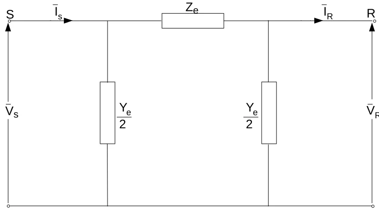
2.5 Transmission Line Modeling

Transmission lines are considered as the carriers of the power from the generating stations

to the load centers. There are different types of transmission lines classified based on

the capability of amount of power transfer, length of the line, the material used for the

construction of the line, e.c.t.,There are four basic elements by which the transmission line is

characterized, they are the series resistance (R), shunt conductance (G), series inductance

(L) and the shunt capacitance (C) of the transmission line.

The voltage and current equations at a distance x from the receiving end of a transposed

distributed parameter line per phase is given as

¯

V = V¯R+ZcI¯R

2 e

γx₊V¯R−ZcI¯R

2 e

−γx _(2.22)

¯

I = ¯

VR/Zc+ ¯IR

2 e

γx₋ V¯R/Zc−I¯R

2 e

−γx

(30)

where

Zc =

p

z/y,

γ =√yz =α+jβ

Zc is the characteristic impedance, γ is called the propagation constant, α is the attenuation

constant, and β is the phase constant.

These equations represents the complete description of the performance of the transmission

lines. This thesis considers only the π-transmission lines, so the equivalent circuit and the π

equivalent circuit of the transmission lines is discussed.

Equivalent circuit model:

In Equation 2.22 and Equation 2.23, by letting x=l and rearranging, we get

¯

VS = ¯VRcosh(γl) +ZcI¯Rsinh(γl) (2.24)

¯

IS = ¯IRcosh(γl) + ¯

VR

Zc

sinh(γl) (2.25)

The equivalent circuit based on the above equations is drawn as in Figure 2.4. Here S, R

represents the sending and receiving end of the transmission line. From the circuit, sending

end voltage is given as

¯

Vs =Ze( ¯IR+

Ye 2

¯

VR) + ¯VR (2.26)

Comparing Equation 2.24 and Equation 2.26, we get

(31)

Z_e ◦

◦

V_s V_R

I_s I_R

Y_e 2

S R

Figure 2.4: Equivalent π transmission line

and

ZeYe

2 + 1 = cosh(γl)⇒

Ye

2 =

1

Zc

tanh(γl

2) (2.28)

If the transmission line is considered negligible i.e., γl1, Ze and Ye can be approximated

as

Ze =Zcsinh(γl)≈Zcγl≈zl =Z (2.29)

and

Ye

2 =

1

Zc

tanh(γl

2)≈

1

Zc

γl

2 ≈

γl

2 =

Y

2 (2.30)

2.6 Load Modeling

Load modeling is one of the important part in terms of modeling a power system. Load is

(32)

generation. There are different types of loads exist in a network, like Industrial, Residential,

Commercial, e.c.t., Each type of load contains different elements such as Induction motors,

Furnaces, Compressors, Refrigerators, Lamps, e.c.t., Not all the loads are constant, there will

be a variation in the load level every hour. As there cannot be any constant load, it becomes

difficult to model a load. In general for planning purposes (load-flow analysis), the load can

be considered as a static load but when the dynamics of the system are included the dynamic

model of the load need to be included.

Static Modeling: A static load model expresses the characteristics of the load at any instant of time as algebraic functions of the bus voltage magnitude and frequency at that

instant. The active and reactive power components are considered separately. Traditionally,

the voltage dependency of load characteristics has been represented by the exponential model

as

P =PO( ¯V)a (2.31)

Q=QO( ¯V)b (2.32)

Here, P and Q are active and reactive components of the load and the voltage ¯V = V

VO, V

is the magnitude of bus voltage. Subscript o indicates the initial operating condition.

The parameters a and b represents constant power, constant current or constant impedance

for the values 0, 1, or 2 respectively. [19] gives the detailed explanation of the alternate

polynomial model which is used to represent the voltage dependency of loads.

(33)

representation of the wide range of characteristics exhibited by the various load components.

The load components that require dynamic load modeling includes induction motors, discharge

lamps, thermostat controlled loads, transformer with saturation, shunt capacitors, e.c.t., The

(34)

Chapter 3 Main Focus and Contribution

3.1 Introduction

The main focus of the thesis is to compare the performance of a test system in real time

against the steady state dynamic analysis. The steady state dynamic analysis is the usual

practice in any electric utility for planning purposes and never performs a real time study

by which the analysis can not be considered precise for the real time operation. In this

thesis the differences are shown by comparing both the real time and steady state dynamic

analysis. Furthermore, a methodology for equating the dynamic performance of the three

software packages (discussed below) by identifying and adjusting the parameters contributing

to output Overshoot, Ripples, and Settling time is introduced. For the comparison purposes,

the power system software used are

• PSS/E - For Steady State Dynamic Analysis

• Hypersim - For Real Time Analysis

• EMTP - For validation purposes

PSS/E:Power System Simulator for Engineering (PSS/E) is a software tool used for electrical

(35)

power system transmission network and generation performance in both steady-state and

dynamic conditions. PSS/E is a high-performance transmission planning software which

supported the power community with meticulous and comprehensive modeling capabilities

since its introduction in 1976.

EMTP:The ElectroMagnetic Transient Program (EMTP) was originally developed by

Professor Hermann W. Dommel in Germany in the late 1960’s [16]. Since then, EMTP has

been continuously developed through international contributions. In 2003, the Development

Coordination Group (DCG) released a new restructured version, EMTP-RV, developed under

the technical leadership of Hydro-Quebec. It features new and improved functionalities, as

well as state-of-the-art analysis tools.

Hypersim: Hypersim is the only real-time digital simulator with the power to simulate and

analyze very large-scale power systems with more than 2000 three-phase buses. Based on

decades of research by Hydro-Quebec on one of the worlds most complex transmission power

systems, Hypersim is an ever-improving solution with a proven track record. Hypersim is

used every day in extremely demanding situations and is constantly updated to increase

performance, reliability and ease of use. As a result, it is rapidly becoming the new standard

for very large power systems.

3.2 Methodology

The methodology of this thesis is based on performing sensitivity analysis of the transfer

function of the excitation system and identifying the parameters for each of the three dynamic

(36)

START

STOP

Power System Raw Data

Build Power System Model in Software

Assign values to the elements

Perform Power Flow Analysis in PSS/E

Compare the Results with Hypersim Load Flow Results

Matched??

YES

Modify the parameter values

NO

Figure 3.1: Flow chart for performing Steady State Analysis

is to be performed prior to performing the Dynamic simulations on any power system when

the power system software packages are used. The flow charts in Figure 3.1 and Figure 3.2

shows the step-by-step procedure for performing, modifying, and analyzing the Steady State

Analysis and Dynamic Analysis respectively. Following two sections clearly describes the

parameter considerations and the proposed methodology for the IEEE-14 Bus Test System

considered in the thesis.

3.3 Steady State Analysis

The steady state phasor models are used for power flow and fault studies. This type of

(37)

START

STOP

Power System Steady State PSS/E Model

Add Generator Dynamics

Assign values to the Exciter Parameters

Perform Dynamic Analysis in PSS/E

Compare the Results with Hypersim Dynamic Simulations

Matched??

YES

Modify the parameter values

NO

Figure 3.2: Flow chart for performing Dynamic Analysis

with impedances and loads, all represented at fundamental frequency. During the steady

state analysis, the power system model is considered as a balanced three-phase system with

balanced voltages and balanced loads. As the system is considered balanced, it becomes easy

for the analysis.

The general procedure of performing the steady state analysis as shown in Figure 3.1

is as follows. First the raw data of the voltage sources, loads, transmission lines, shunt

capacitors, transformers of a desired test system is considered as the base for the steady

state analysis. Then the single line diagram of the test system is to be modeled in the power

system software package. After building the model, the previously considered values are

assigned and then load flow analysis is to be performed on the system. If the results from

(38)

else the parameters of the network elements are modified accordingly such that the power

flow results like Bus voltage magnitudes, Bus voltage angles, Active power flow, Reactive

power flow matches.

In the thesis, IEEE-14 Bus system is considered as the test system and the test data is

shown in chapter 4. The test data is assigned to the models built in PSS/E, EMTP, and

Hypersim on which the power flow/load flow analysis (Newton Raphson method is used) is

performed. The results obtained from the three software packages is then compared. The

results are shown in chapter 5. In the present case, the steady state analysis results were

matched without any modifications of the parameters.

3.4 Dynamic Analysis

The dynamic analysis models uses a series of solved power flow cases with appropriate

adjustment of the system’s dynamic parameters between each power flow calculation. So the

first step in matching the dynamic response among the three platforms is to add a dynamic

element with its dynamic parameters. For the thesis dynamic generator model is considered

in the test case.

The procedure for the dynamic analysis considers the power flow model of the test case

as the base. A dynamic element on which the analysis is to be performed is added to the

base case. Appropriate parameters are assigned to the dynamic element and the dynamic

analysis is performed where the results are captured and compared with that obtained from

the other software packages. If the results are not quite similar, the parameters are to be

(39)

In the thesis, PSS/E analysis is considered as the reference for the results. After matching

the steady state results, the dynamics of a synchronous generator (GENROU) along with the

excitation system (IEEE Type-1) is added to the case under consideration. A three-phase

bus fault is applied on the system to see the response of the generator and the excitation

system. The windowed rms values of the bus voltages at the desired buses are captured

and are overlapped with the one obtained from the other two software packages. A large

difference is observed between PSS/E and EMTP, Hypersim when considered as a package

since EMTP and Hypersim gives similar results. So the parameters of the excitation system

of the generator are tweaked carefully so that the resulting waveform of the desired buses

matches with the one obtained from EMTP, Hypersim.

The details of the generator models, the procedure for tweaking the parameters is discussed

in the following sections.

EMTP and Hypersim can generate voltages even with the static voltage source whereas

PSS/E cannot run dynamics on any network without a dynamic model. Therefore, it is

mandatory to add dynamic models in the test case. Dynamic modeling of a generator is

considered here which includes

• Rotor model

• Excitation system model

• Governor model

• Stabilizer model

(40)

are slow in reacting to the sudden changes (faults) in the system and does not respond

quickly for the electromagnetic transients during faults, the governor and stabilizer models

are ignored. From generator rotor and exciter models, as the excitation system parameters

are tweaked, the procedure for the selection of the parameters to be tweaked, the exciter

transfer function, the sensitivity ranking of the parameters are required for finding the most

sensitive parameter for a small change in the system. This analysis is considered as the most

important part of the thesis as this simplifies the selection of the parameter to be tweaked.

The following section covers the calculation of the transfer function of the exciter, then follows

the sensitivity analysis.

3.4.1 Exciter Transfer Function

The exciter used in this thesis is IEEE Type-1 as shown in Figure 3.3. Transfer function i.e.,

input-output relationship of the excitation system is calculated in the present section for the

detailed study of sensitivity analysis of the system. IEEE Type-1 excitation system is one of

the 63 types of exciters approved by IEEE [9]. However, we have selected IEEE Type-1 to be

compatible with the software used for modeling and simulation of an actual electric utility

topology. The transfer function of the block diagram of Figure 3.3 is calculated as shown in

the following paragraphs. As the control block has more than one input, according to [15]

the transfer function is the algebraic sum of the transfer functions obtained by individual

inputs when the other inputs set to zero. This statement is valid only when the step response

(in S-domain) is to be obtained. As the three inputs for the excitation system in the thesis

(41)

step response of the excitation system is also shown and is verified with Matlab Simulink. In

the following calculations, first Ec alone is considered assumingVRef and Vs as zeros and is

followed by VRef and Vs.

Figure 3.3: IEEE Type-1 Exciter Block Diagram [9]

where

TR - Transducer time constant in Seconds

TA - AVR time constant in Seconds

TE - Exciter time constant in Seconds

TF - Field voltage feedback time constant in Seconds

KA - AVR gain in pu

(42)

KF - Field voltage feedback gain in pu

VRM ax - AVR limit max in pu

VRM in - AVR limit min in pu

E1 - Saturation voltage at point 1 in pu

E2 - Saturation voltage at point 2 in pu

S(E1) - Saturation atE1 in pu

S(E2) - Saturation atE2 in pu

Input: Ec

Step-1: Consider the blocks with gain KE and SE of the excitation voltage model. Here

though SE is a saturation function which is not a constant, we consider a value at particular

instant for the calculation of the transfer function and performing sensitivity analysis.

y1 =KE +SE (3.1)

Step-2: Consider the blocks with gain y1 and _sTE1 .

y2 =

1 sTE 1 + (_sTE1 ∗y1)

y2 =

1 sTE

1 + (_sTE1 ∗(KE +SE))

y2 = 1

sTE +KE +SE

(43)

Step-3: Consider the blocks with gain y2 and ₁₊KA_sTA.

y3 = KA

1 +sTA

∗ 1

sTE +KE+SE

(3.3)

Step-4: Consider the blocks with gain y3 and sKF

1+sTF.

y4 = y3 1 + ( sKF

1+sTF ∗y3)

y4 = KA∗(1 +sTF)

((1 +sTA)(1 +sTF)(sTE +KE+SE)) +KAsKF

(3.4)

Step-5: Consider the blocks with gain y4 and (− 1

1+sTR).

y5 = (− 1

1 +sTR

)∗y4

T.F1 =

−KA∗(1 +sTF)

(1 +sTR)∗(((1 +sTA)(1 +sTF)(sTE+KE +SE)) +KAsKF)

(3.5)

Input: VRef

The process of the reduction of the block diagram with VRef is the same as with Ec. Repeat

the steps 1 through 4 and the transfer function with VRef is given by Equation 3.6 which is

same as that in Equation 3.4.

T.F2 =

KA∗(1 +sTF)

((1 +sTA)(1 +sTF)(sTE +KE +SE) +KAsKF)

(44)

Input: VS

The process of the reduction of the block diagram with VS is the same as with Ec. Repeat

the steps 1 through 4 and the transfer function with VS is given by Equation 3.7 which is

same as that in Equation 3.4.

T.F3 =

KA∗(1 +sTF)

((1 +sTA)(1 +sTF)(sTE +KE +SE) +KAsKF)

(3.7)

Therefore, the total transfer function relating input-output of the excitation system

block diagram assuming all the three inputs are the same and has a magnitude one is the

combination of Equation 3.5, Equation 3.6 and Equation 3.7 and is given by Equation 3.8.

G(s) = Y(s)

U(s) =

KA∗(1 +sTF)∗(1 + 2sTR)

(1 +sTR)∗(((1 +sTA)(1 +sTF)(sTE+KE +SE)) +KAsKF)

(3.8)

The overall transfer function shown in Equation 3.8 is verified using Matlab Simulink.

Figure 3.4 and Figure 3.5 shows the actual block diagram of the IEEE Type-1 exciter with all

the inputs set to one and the output respectively. Figure 3.6 and Figure 3.7 are the overall

transfer function obtained in Equation 3.8 with a step input and the output of the transfer

function block respectively. In both the cases, a set of parameters are chosen and from the

results it is clearly seen that both the blocks gives the same output which verifies that the

calculation of the transfer function of the excitation system is accurate.

As discussed earlier in this section, the overall transfer function shown in Equation 3.8 is

not considered for the sensitivity analysis. As the overall transfer function for this exciter

(45)

and the clarification on the sensitivity analysis of the particular excitation system is given in

subsection 3.4.2.

Figure 3.4: Transfer function block diagram with three step inputs

3.4.2 Sensitivity Analysis of Excitation System

The sensitivity analysis of a function F(s) with respect to a parameter k can be defined as

the percent change in the function, F(s) to the percent change in the parameter, k. This

analysis basically reveals how sensitive is the gain of the transfer function to the changes of

a particular parameter. The larger the magnitude of the transfer function gain, the more

sensitive is the parameter. The sensitivity function can be written as

S_kF(s) = %changeinF(s) %changeink

S_kF(s,k) = ∂F(s, k)/F(s, k)

(46)

Figure 3.5: Output of the transfer function block diagram with three step inputs

(47)

Figure 3.7: Output of the overall transfer function with a step input

Equation 3.9 can also be written as

S_kF(s,k) = ∂lnF(s, k)

∂lnk (3.10)

where ln represents the natural log of the variable. From the basics, we know that

F(s, k) = N(s, k)

D(s, k) (3.11)

Substituting Equation 3.11 in Equation 3.10 and rearranging, we get

S_kF(s,k) = ∂lnN(s, k)

∂lnk −

∂lnD(s, k)

(48)

Using Equation 3.10, Equation 3.12 can be rewritten as

S_kF(s,k) =S_kN(s,k)−S_kD(s,k) (3.13)

In Equation 3.13 if the numerator or the denominator of F(s,k) is not a function of the

parameter k, the corresponding sensitivity in the right hand side of Equation 3.13 will vanish.

Also note that the sensitivity of Equation 3.13 depends on both the frequency s=σ+jω and

the parameter k. To quantify the measure of sensitivity, Equation 3.13 is evaluated at a

specific frequency s=s0 and at the nominal value of the parameterk =k0.

For the closed loop system, Equation 3.13 can be used with the appropriate numerator

and denominator functions. With the feedback function, H(s)6=0, the transfer function is

written as shown in Equation 3.14

T(s, k) = G(s, k)

1 +G(s, k)H(s, k) (3.14)

If there are any poles in the transfer function of Equation 3.14 that gives negative sign

in the sensitivity analysis, that indicates that the gain of the transfer function reduces as

the parameter is increased. However with the increase of this pole, the stability of the

system is increased while reducing the transfer function gain. When a parameter appears

in both numerator and the denominator of the closed-loop transfer function, changing the

parameter may cause a change in the magnitude of the transfer function while at the same

time impacting transient and steady-state response of the system including system stability,

(49)

metrics which may be used to quantify performance of a system in steady-state or while

in transient to a new operating state and they are all based on optimizing a performance

measure corresponding to different design criterion or operating conditions. Often using a

metric for minimizing the steady-state error of a system will cause undesired transients by

introducing a more oscillatory response. So while considering a sensitivity analysis on any

system model with parameters in both numerator and denominator and Equation 3.13 is to

be applied on the system, we may place the parameters into different categories if they are

independent from each other. This would simplify the sensitivity analysis. However if the

parameters are dependent, then we may observe changes in both steady state and transient

response of the system impacting system overshoot, oscillations, and or settling time.

As discussed earlier in this chapter,the transfer function of the exciter considered in this

thesis cannot be written as an input output relation. So the transfer function which has high

impact on the overall control block and in turn on the test system is considered. In this case

the transfer function related to the input EC (Equation 3.5) is considered the most effective

transfer function. Now the sensitivity analysis is applied on this transfer function. Though

this transfer function cannot give the exact ranking of the parameters, they can be grouped

into different categories by comparing the effect of the variation of the parameters obtained

by the software simulations with the calculated sensitivities. There are 7 parameters in the

transfer function (considering saturation function is not present for simplicity) which are

varied one at a time and find both the sensitivity from the calculations and that obtained

from plots. Here EMTP simulations are considered for the sensitivity analysis.

The parameters [22] shown in Table 3.1 are used for finding the sensitivity of the exciter

(50)

Table 3.1: Parameter values for calculating sensitivity

Parameter Value

KA 400

TA 0.05

TE 0.95

KE -0.17

KF 0.04

TF 1.00

TR 0.00

SE 0.00

By varying one parameter at a time and calculating the sensitivity, the ranking of the

parameters is given as shown in Table 3.3. Here all the parameters are varied according

to the range of the parameters shown in obtained from [1]. Hundred values are considered

within the range of the parameter values and out of the hundred different sensitivity ranking,

the rank for a particular parameter occuring highest number of times is considered as its

rank and the resulting parameter rankings are as given in Table 3.3.

Table 3.2: Parameter’s range for the sensitivity analysis

Rank Parameter

1 0 ≤TR <0.5

2 10 < KA < 500

3 0≤ TA <1

4 -1 ≤KE ≤ 1

5 0.04 < TE <1 6 0< KF < 0.3 7 0.04 < TF < 1.5

8 5 ≤TF/KF ≤ 15

From the 100 calculations of sensitivities, bothTF andKF shared rank 1 but asTF ranked

1 a little more number of times, it is considered as Rank-1. Though they are considered in

(51)

Table 3.3: Parameter Ranking based on Sensitivity

Rank Parameter

1 TF

2 KF

3 KA

4 TE

5 KE

6 TA

7 TR

are considered in the third group. For the validation of these groupings and the sensitivity

analysis, the simulations are performed in EMTP by varying the parameters of the exciter.

The response of the system voltages to the fault with the variation in the parameters are

captured. These are grouped according to the effect of the variation of the parameter value

on overshoot, oscillations and/or the settling time.

V_1 [Spreadsheet1]V_1 [Spreadsheet2]V_1 [Spreadsheet3]

7.2 7.6 8 8.4 8.8 9.2 9.6 10 10.4 10.8

Time (s) 0.4 0.6 0.8 1 1.2 V oltage (V)

7.2 7.6 8 8.4 8.8 Time (s) 9.2 9.6 10 10.4 10.8

0.4 0.6 0.8 1 1.2 Voltage (V)

7.2 7.6 8 8.4 8.8 9.2 9.6 10 10.4 10.8

Time (s) −0.4 0 0.4 0.8 1.2 V oltage (V)

[Spreadsheet1] T_F_0.5 − E:\Individual\sowmya\Thesis_04_04_2016_EMTP\EMTP_T_F [Spreadsheet2] T_F_1.4 − E:\Individual\sowmya\Thesis_04_04_2016_EMTP\EMTP_T_F [Spreadsheet3] original_T_F_1 − E:\Individual\sowmya\Thesis_04_04_2016_EMTP\EMTP_T_F

Printed for p 1

Figure 3.8: Variation of TF; Voltage at

Bus 1, Bus 2, Bus 3 (in pu) with respect to time

7.2 7.6 8 8.4 8.8 9.2 9.6 10 10.4 10.8

Time (s) 0.4 0.6 0.8 1 1.2 V oltage (V)

7.2 7.6 8 8.4 8.8 Time (s) 9.2 9.6 10 10.4 10.8

0.4 0.6 0.8 1 1.2 Voltage (V)

7.2 7.6 8 8.4 8.8 9.2 9.6 10 10.4 10.8

Time (s) −0.4 0 0.4 0.8 1.2 V oltage (V)

[Spreadsheet1] K_F_0.1 − E:\Individual\sowmya\Thesis_04_04_2016_EMTP\EMTP_K_F [Spreadsheet2] K_F_0.25 − E:\Individual\sowmya\Thesis_04_04_2016_EMTP\EMTP_K_F [Spreadsheet3] original_K_F_0.04 − E:\Individual\sowmya\Thesis_04_04_2016_EMTP\EMTP_K_F

Printed for p 1

Figure 3.9: Variation of KF; Voltage at

The graphs shown in the Figure 3.8 through Figure 3.14 are the windowed rms voltages

of Bus-1, Bus-2, and Bus-3 with a short circuit fault applied on Bus-3. Three different values

(52)

7.2 7.6 8 8.4 8.8 9.2 9.6 10 10.4 10.8

Time (s) 0.4 0.6 0.8 1 1.2 V oltage (V)

7.2 7.6 8 8.4 8.8 9.2 9.6 10 10.4 10.8

Time (s) 0.4 0.6 0.8 1 1.2 Voltage (V)

7.2 7.6 8 8.4 8.8 9.2 9.6 10 10.4 10.8

Time (s) −0.4 0 0.4 0.8 1.2 V oltage (V)

[Spreadsheet1] K_A_100 − E:\Individual\sowmya\Thesis_04_04_2016_EMTP\EMTP_K_A [Spreadsheet2] K_A_250 − E:\Individual\sowmya\Thesis_04_04_2016_EMTP\EMTP_K_A [Spreadsheet3] original_K_A_400 − E:\Individual\sowmya\Thesis_04_04_2016_EMTP\EMTP_K_A

Printed for p 1

Figure 3.10: Variation of KA; Voltage at

7.2 7.6 8 8.4 8.8 9.2 9.6 10 10.4 10.8

Time (s) 0.4 0.6 0.8 1 1.2 V oltage (V)

7.2 7.6 8 8.4 8.8 9.2 9.6 10 10.4 10.8

Time (s) 0.4 0.6 0.8 1 1.2 Voltage (V)

7.2 7.6 8 8.4 8.8 9.2 9.6 10 10.4 10.8

Time (s) −0.4 0 0.4 0.8 1.2 V oltage (V)

[Spreadsheet1] T_E_0.05 − E:\Individual\sowmya\Thesis_04_04_2016_EMTP\EMTP_T_E [Spreadsheet2] T_E_0.5 − E:\Individual\sowmya\Thesis_04_04_2016_EMTP\EMTP_T_E [Spreadsheet3] original_T_E_0.95 − E:\Individual\sowmya\Thesis_04_04_2016_EMTP\EMTP_T_E

Printed for p 1

Figure 3.11: Variation of TE; Voltage at

7.2 7.6 8 8.4 8.8 9.2 9.6 10 10.4 10.8

Time (s) 0.4 0.6 0.8 1 1.2 V oltage (V)

7.2 7.6 8 8.4 8.8 Time (s) 9.2 9.6 10 10.4 10.8

0.4 0.6 0.8 1 1.2 Voltage (V)

7.2 7.6 8 8.4 8.8 9.2 9.6 10 10.4 10.8

Time (s) −0.4 0 0.4 0.8 1.2 V oltage (V)

[Spreadsheet1] K_E_0 − E:\Individual\sowmya\Thesis_04_04_2016_EMTP\EMTP_K_E [Spreadsheet2] K_E_0.5 − E:\Individual\sowmya\Thesis_04_04_2016_EMTP\EMTP_K_E [Spreadsheet3] original_K_E_−0.17 − E:\Individual\sowmya\Thesis_04_04_2016_EMTP\EMTP_K_E

Printed for p 1

Figure 3.12: Variation ofKE; Voltage at

7.2 7.6 8 8.4 8.8 9.2 9.6 10 10.4 10.8

Time (s) 0.4 0.6 0.8 1 1.2 V oltage (V)

7.2 7.6 8 8.4 8.8 Time (s) 9.2 9.6 10 10.4 10.8

0.4 0.6 0.8 1 1.2 Voltage (V)

7.2 7.6 8 8.4 8.8 9.2 9.6 10 10.4 10.8

Time (s) −0.4 0 0.4 0.8 1.2 V oltage (V)

[Spreadsheet1] T_A_0 − E:\Individual\sowmya\Thesis_04_04_2016_EMTP\EMTP_T_A [Spreadsheet2] T_A_0.1 − E:\Individual\sowmya\Thesis_04_04_2016_EMTP\EMTP_T_A [Spreadsheet3] original_T_A_0.05 − E:\Individual\sowmya\Thesis_04_04_2016_EMTP\EMTP_T_A

Printed for p 1

Figure 3.13: Variation of TA; Voltage at

observing the graphs closely, they are grouped as following.

• TF,KF - Overshoot

• KA, TE - Oscillations

• KE,TA, and TR - Slight Overshoots, Slight Settling time.

From the plots and the grouping, it is clear that the transfer function considered has a high

Sensitivity Analysis of Synchronous Generators for Real-Time Simulation

ScholarWorks@UNO

ScholarWorks@UNO

Sensitivity Analysis of Synchronous Generators for Real-Time

Sensitivity Analysis of Synchronous Generators for Real-Time

Simulation

Simulation

Sensitivity Analysis of Synchronous Generators for Real-Time

Simulation

A Thesis

Submitted to the Graduate Faculty of the

University of New Orleans

in partial fulfillment of the

requirements of the degree of

Master of Science

in

Engineering

Electrical Engineering

By

Sowmya Munukuntla

B-Tech. Jawaharlal Nehru Technological University, 2012

Acknowledgement

Contents

List of Figures

List of Tables

Abstract

Chapter 1

Problem Statement and Historical

Review

1.1

Introduction

1.2

Types of Models

1.2.1

Application of generator models in stability studies

1.3

Historical Background

1.3.1

Scope of Work

Chapter 2

Mathematical Background

2.1

Introduction

2.2

Generator Modeling

2.3

Exciter Modeling

2.4

Transformer Modeling

v

v

ᵒ

ᵒ

ᵒ

ᵒ

Z

Z

i

i

-v

-

-v

n

:

n

P

S

-n

-

-

-

n

- -

2.5

Transmission Line Modeling

2.6

Load Modeling

Chapter 3

Main Focus and Contribution

3.1

_i