R E S E A R C H A R T I C L E
Open Access
Auxiliary variables in multiple imputation in
regression with missing X: a warning against
including too many in small sample research
Jochen Hardt
1*, Max Herke
1and Rainer Leonhart
2Abstract
Background:Multiple imputation is becoming increasingly popular. Theoretical considerations as well as simulation studies have shown that the inclusion of auxiliary variables is generally of benefit.
Methods:A simulation study of a linear regression with a response Y and two predictors X1andX2was performed on data with n = 50, 100 and 200 using complete cases or multiple imputation with 0, 10, 20, 40 and 80 auxiliary variables. Mechanisms of missingness were either 100% MCAR or 50% MAR + 50% MCAR. Auxiliary variables had low (r=.10) vs. moderate correlations (r=.50) with X’s and Y.
Results:The inclusion of auxiliary variables can improve a multiple imputation model. However, inclusion of too many variables leads to downward bias of regression coefficients and decreases precision. When the correlations are low, inclusion of auxiliary variables is not useful.
Conclusion:More research on auxiliary variables in multiple imputation should be performed. A preliminary rule of thumb could be that the ratio of variables to cases with complete data should not go below 1 : 3.
Keywords:Multiple imputation, Auxiliary variables, Simulation study, Small and medium size samples
Background
Missing data in statistical analyses is the rule rather than the exception. Many statistical methods can only analyse cases with complete data, so a way to deal with the miss-ing data needs to be found. The traditional approach was to only use cases complete data for the variables of interest is fully available, which is often referred to as the Complete Cases analysis (CC). However, not only is CC inefficient when models with many variables are to be examined, it can also introduce bias to regression coefficients when the mechanism that leads to missing data is anything other than missing completely at random [MCAR: 1]. Multiple imputation (MI) was introduced in the 1970s as a way to deal more efficiently with missing data [2]. It met with small to moderate resonance at first, but since 2008, Mackinnon [3] has observed a drastic in-crease in articles on applying multiple imputation to data
analyses published in four leading medical journals (BMJ, JAMA, Lancet, NEJM). However, CC is still utilized in the majority of publications–Karahaliouset al.[4] reviewed the methods utilized in prospective cohort studies with samples larger than n=1000 published during the first ten years of the century: of 82, only 5 utilized MI.
Basically, MI creates multiple datasets that are copies of the original complete data. The missing observations in these datasets are then imputed, using a stochastic al-gorithm that estimates values based on information con-tained within the observed values and creates different values in each dataset. The additional variance caused by differences in the imputed values between the various copies reflects the uncertainty of the imputation. The relative increase of variance due to substitution of miss-ing data can be calculated for any given data [5]. Statis-tics are performed separately for these datasets and coefficients are combined at the conclusion of the ana-lysis [5]. Finally, the degrees of freedom are adjusted. MI leads to results without bias for many missing at random [MAR: 1] conditions that introduce bias in CC, but there
* Correspondence:[email protected]
1Medical Psychology and Medical Sociology, Clinic for Psychosomatic
Medicine and Psychotherapy, University of Mainz, Duesbergweg 6, Mainz 55128, Germany
Full list of author information is available at the end of the article
are also situations in which MI produces bias and CC does note.g.[6,7].
In most cases, it has been demonstrated that MI is su-perior to CC and various other ways of dealing with missing datae.g.[8]. This has been proven in large sam-plese.g.[9,10] or when data in the response variables is missing, for example when there are dropouts in
repeated measurement designs e.g. [11]. In the latter
case, variables from different points in time are often highly correlated, enabling MI algorithms to generate good results. In such complex responses consisting of many correlated variables, substitution of missing data generally improves parameter estimation. When missing data occurs in a single response (typically analysed within the general linear model), any way of substituting a response will introduce noise rather than being helpful if auxiliary variables are not used [12].
An additional advantage of MI over CC is the possi-bility of including information from auxiliary variables into the imputation model. Auxiliary variables are vari-ables within the original data that are not included in the analysis, but are correlated to the variables of inter-est or help to keep the missing process random [MAR: 1]. Little [6] has calculated the amount of decrease in
variance of a regression coefficient Y on X1 when a
covariate X2 is added that has no missing data. White
and Carlin [7] have extended this proof to more than one covariate. In practice however, it is likely that auxil-iary variables themselves will have missing data. Collins et al. [13] performed a simulation study in which they tested the influence of auxiliary variables with missing data in a regression model. Particularly good results were obtained by including auxiliary variables when (a) the missing data were in the response, (b) the auxiliary vari-able changed the process leading to missing data from
“missing not at random” (MNAR) to MAR and when
(c) the correlation of the auxiliary variable to the response was very high, i.e. r=.9. In their study, the information gained due to auxiliary variables was generally larger than the noise that was introduced by irrelevant information. For this reason, they recommended using inclusive rather than restrictive strategies.
This is in line with recommendations by most experts: the imputation model should include all variables of the analysis, plus those highly correlated with responses or explanatory variables, and finally those variables that ex-plain the mechanism leading to missing datae.g. [2,14]. Enders [15, p. 127ff] demonstrated that when an auxil-iary variable which mediates between an outcome Y and an explanatory variable X is not included in the substitu-tion model, some bias in the estimates occurs and the power of the analyses decreases.
Another simulation study explored the role of aux-iliary variables in confirmatory factor analysis and also
concluded that the inclusion of auxiliary variables is beneficial [16]. However, from a practical point of view, inclusion of too many variables leads to a considerable increase in computation time or even causes programs to fail [17]. The latter happens with continuous linear vari-ables in most programs when the number of varivari-ables approaches the number of cases. In the study by Collins et al. [13], the ratio of subjects to included variables
never fell below 10 to 1 – although this could easily
occur in small sample research. For example, if a re-searcher had 100 subjects in a questionnaire survey com-prising 10 scales based on six items each plus some demographics, there would be more than 60 variables on the item basis and about sixteen variables on the scale basis. Repeated measurement designs may have even
more variables e.g. [18]. However, these face different
problems that will not be addressed here.
The aim of the present paper is to simulate various realistic situations that might occur in a medical survey. Within this frame, we have explored the effect of using auxiliary variables in the substitution model for missing data in explanatory variables of a linear regression model. A model was chosen with a response Y with two correlated continuous predictors X1and X2, both show-ing strong associations to Y total R2= .40: [19]. Varying proportions of missing data were introduced into this model and analyses using CC and MI were applied, the latter with varying numbers of auxiliary variables. To il-lustrate, an example is provided where data is missing from the items of a questionnaire scale.
Method
Simulation design
The analysis parameter was the non-standardized b1
-coefficient from the following formula:
Y¼αþb1X1þb2X2þe;
50% of the observations in the X1, X2, and Za variables were deleted by (v) one of three mechanisms.
MCAR
Observations in X1, X2 and Za were deleted completely at random.
MAR(Y)
No full MAR mechanism was applied here, because in real data, finding a variable that completely explains the process of missingness is unlikely. Thus, the observa-tions to be deleted in X1, X2 and Za were chosen de-pending on the unweighted sum of a random standard normal distribution and the standard normal distribu-tion of Y, with the highest sums introducing missing data in X1, X2 and Za. In terms of Allison (2000), this
mechanism consists of “50% MCAR and 50% MAR
(dependent on Y)”.
MAR(X)
A procedure similar to the one utilized in MAR(Y), but
the observations of X1 and Za were deleted depending
on the sum of X2 and a value from a random normal
distribution; the observations ofX2depended on X1and
a value from a random normal distribution. Since X1
and X2have a standard normal distribution as well, this
results in“50% MCAR and 50% MAR(dependent on X)”
as defined by Allison (2000). Again, the highest values introduced the missing data.
The generating process for MAR(Y) was:
After z-transformation of Y, let all X1,X2, Y and c be X1,X2, Y, c ~ N(0,1)
Summing:d=Y+c
Ranking: dj< dkfor each i, j from N
Deleting: X1,X2, Zais missing if d≥h: for h = 4%, 8%. . .64%
Similar for MAR(X):
Let all X1,X2, Y, Za, c ~ N(0,1) Summing:d1=X2+c,d2=X1+c Ranking: dj< dkfor each i, j from N
Deleting: X1,Zaif d1≥h: for h = 4%, 8%. . .64% X2if d2≥h: for h = 4%, 8%. . .64%
No MNAR condition was created, and no observations of Y were deleted in the present study. The deletion of observation was carried out separately for each variable. This means that there were cases in the analyses that had no observed values for X1and X2as well as for Za, only multiply imputed values. At first sight, one may question whether this makes sense. However, in a com-plex analysis where various regression analyses are
involved (e.g.searching for a mediator), this could be ne-cessary. Hence, our simulations encompassed this possibility.
Using multiple imputations by chained equations, m = 20 imputed data sets were created [1]. There was a recommendation by Little and Rubin that creating three to five data sets is usually enough. In more recent articles, probably due to increasing computational power, this recommendation has changed, suggesting the use of a greater number of imputed datasets in real
data analyses, i.e. 20 – 100 [17,22,23]. Values were
imputed via chained equations followed by predictive
mean matching (PMM) using the program “MICE”
[24,25]. This combination was chosen because it yielded the best results in previous simulation studies [26,27].
The combination of (i) three sample sizes, (ii) ten ways of handling missing data including the two levels of cor-relations (r=.1 or r=.5) in the auxiliary variables, (iv) two percentages of missing observations and (v) three mechanisms for deleting data resulted in 180 different simulations. The simulations were conducted with q=1000 replications each. Each simulation was started with a random seed and created different seeds for each replication for use with the random number generator. For each replication, a new complete dataset was gener-ated, and then the intended percentage of data was deleted. Depending on the simulated condition, this was either directly followed by fitting the linear regression model using the CC method, or by first creating multiple imputations and then following with regression analyses. The latter were conducted separately on each data set and pooled applying Rubin’s Rules. For the b1-coefficient, the raw bias (mean of estimated – true coefficient), its standard error (SE), the standardized bias (raw bias/SE) as well as the root mean square error (RMSE) over the q=1000 replications (i.e. qffiffiffiffiffiffiffiffiffiffiffiffiðbibq Þ2 as an estimate for pre-cision (biis the estimated b-coefficient for replication i, b
the coefficient in the complete data, i.e. 1, and q the
number of replications) are displayed in Tables 1, 2, 3. The presentation of results was oriented on Lee and Carlin’s [28], but the parameter for precision, coverage, was replaced by the RMSE.
Data generation and selection of program parameters
Data was generated in three steps. First, X1andX2were created in random order, drawn from a normal distribu-tion. Second, Y was generated by drawing from a normal distribution, setting b1 and b2-coefficients to 1, then obtaining the necessary errors and adding those to Y so that an R2 of .40 could be created. Third, the auxiliary variables Z were created in random order. Using the Choleski factorization, the variables were transformed to show the desired correlation matrix (all coefficients r = .1 or .5) was generated.
All simulations were performed using R [29]. The simulation data were generated utilizing R's methods for generating random, normally distributed variables, ap-plying the Choleski factorization and solving systems of linear equations [rnorm, chol, solve: 30], all taken from the base and stats packages. R's default random number generator "Mersenne-Twister" was used. The seeds used for each simulation were true random numbers provided
by random.orgviathe package“random”
[randomNum-bers: 31]. Multiple imputation was also performed in R using the package MICE V2.0: [25]. The script used to create the simulation data, induce missing data and per-form multiple imputations and regression analyses can be obtained from the authors.
Results
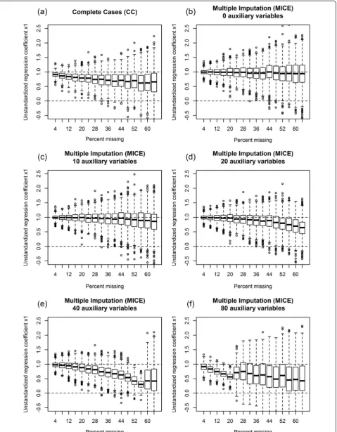
Figure 1 displays the non-standardized regression
coef-ficient b1 under MAR(Y) and n=100. It illustrates the
curve that occurs with increasing amounts of missing data with various numbers of auxiliary variables. The horizontal axis of the graph stands for the percentage of missing data; the vertical axis displays the
distribu-tions of the coefficient b1 over the 1000 replications
for each proportion of missing data. The box-and-whisker plots display the box as the usual 25%, 50%,
and 75%-quantiles of b1 with the whisker having a
maximum of 1.5 times the length of the box. Outlier values of b1 are displayed as circles. The line at value 1 represents the true regression coefficient when there are no missing data. All auxiliary variables in Figure 1
have moderate correlations of r=.5 to X1, X2, Y and
all Z.
Figure 1a displays the results of the CC analysis. A downward bias is clearly visible with increasing rates of missing values, as well as a decrease in precision. Figure 1b shows the same simulation after multiple imputations without any auxiliary variables, i.e. only Y,
X1 and X2 are in the imputation model (MI+0).
Com-pared to CC, there was almost no bias and precision was minimally higher.
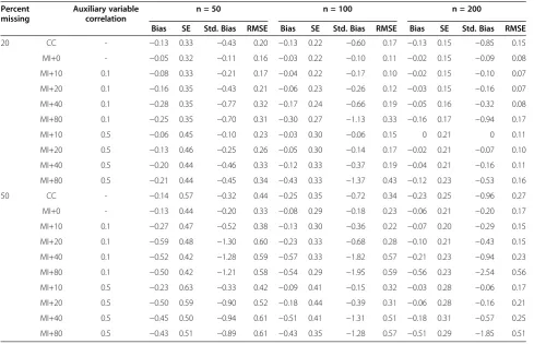
Table 1 Results of the simulations on linear regressions, MAR(Y)
Percent missing
Auxiliary variable correlation
n = 50 n = 100 n = 200
Bias SE Std. Bias RMSE Bias SE Std. Bias RMSE Bias SE Std. Bias RMSE
20 CC - −0.13 0.33 −0.43 0.20 −0.13 0.22 −0.60 0.17 −0.13 0.15 −0.85 0.15
MI+0 - −0.05 0.32 −0.11 0.16 −0.03 0.22 −0.10 0.11 −0.02 0.15 −0.09 0.08
MI+10 0.1 −0.08 0.33 −0.21 0.17 −0.04 0.22 −0.17 0.10 −0.02 0.15 −0.10 0.07
MI+20 0.1 −0.16 0.35 −0.43 0.21 −0.06 0.23 −0.26 0.12 −0.03 0.15 −0.16 0.07
MI+40 0.1 −0.28 0.35 −0.77 0.32 −0.17 0.24 −0.66 0.19 −0.05 0.16 −0.32 0.08
MI+80 0.1 −0.25 0.35 −0.70 0.31 −0.30 0.27 −1.13 0.33 −0.16 0.17 −0.94 0.17
MI+10 0.5 −0.06 0.45 −0.10 0.23 −0.03 0.30 −0.06 0.15 0 0.21 0 0.11
MI+20 0.5 −0.13 0.46 −0.25 0.26 −0.05 0.30 −0.14 0.17 −0.02 0.21 −0.07 0.10
MI+40 0.5 −0.20 0.44 −0.46 0.33 −0.12 0.33 −0.37 0.19 −0.04 0.21 −0.16 0.11
MI+80 0.5 −0.21 0.44 −0.45 0.34 −0.43 0.33 −1.37 0.43 −0.12 0.23 −0.53 0.16
50 CC - −0.14 0.57 −0.32 0.44 −0.25 0.35 −0.72 0.34 −0.23 0.25 −0.96 0.27
MI+0 - −0.13 0.44 −0.20 0.33 −0.08 0.29 −0.18 0.23 −0.06 0.21 −0.20 0.17
MI+10 0.1 −0.27 0.47 −0.52 0.38 −0.13 0.30 −0.36 0.22 −0.07 0.20 −0.29 0.15
MI+20 0.1 −0.59 0.48 −1.30 0.60 −0.23 0.33 −0.68 0.28 −0.10 0.21 −0.43 0.15
MI+40 0.1 −0.52 0.42 −1.28 0.59 −0.57 0.33 −1.82 0.57 −0.21 0.23 −0.94 0.23
MI+80 0.1 −0.50 0.42 −1.21 0.58 −0.54 0.29 −1.95 0.59 −0.56 0.23 −2.54 0.56
MI+10 0.5 −0.23 0.63 −0.33 0.42 −0.09 0.41 −0.15 0.32 −0.03 0.28 −0.06 0.17
MI+20 0.5 −0.50 0.59 −0.90 0.52 −0.18 0.44 −0.39 0.31 −0.06 0.28 −0.16 0.21
MI+40 0.5 −0.45 0.50 −0.94 0.61 −0.51 0.41 −1.31 0.51 −0.18 0.31 −0.57 0.25
Figure 1c displays the situation when ten auxiliary variables were added (MI+10). Here, a slight downward trend of the coefficient could be observed when the missing rate exceeded 40%. Precision was somewhat bet-ter than in MI+0. Figure 1d displays the same simulation with 20 auxiliary variables (MI+20). Up to a missing data rate of 20%, bias was small and precision did not im-prove compared to MI+10. However, with higher rates of missing data, bias increased. Figures 1e and f display the results after inclusion of 40 and 80 auxiliary vari-ables, respectively. They clearly indicate that the inclu-sion of too many variables did not improve the imputation process under these conditions; rather, it was disadvantageous. The inclusion of 40 variables may be acceptable when very few data (<10%) are missing, but it was clearly worse than using less auxiliary variables. The inclusion of 80 auxiliary variables did not make sense in this simulation; when 8% of the data was missing, there was already an extreme bias so that an analysis per-formed on that data set would be seriously impaired by the multiple imputation.
Table 1 displays the results of the main simulations under MAR(Y). The first column under each sample size displays the raw bias of b1over q = 1000 replications. It ranges between zero and -.59 in these simulations, no
upward bias was observed, here. Raw bias was not posi-tively affected by the inclusion of auxiliary variables in these simulations except for one case: 50% missing data, n=200 and 10 auxiliary variables, where it is reduced from -.06 for MI+0 to -.03 for MI+10. The second col-umn displays its standard error (SE) which decreases with the sample size and increases with the number of auxiliary variables. The third column displays the stan-dardized bias, i.e.the ratio of the former two. With few exceptions, the standardized bias increases with the number of auxiliary variables, indicating that including auxiliary variables is not beneficial in these simulations. The exceptions are: ten auxiliary variables with a correl-ation of r = .5 for n = 50, 100, and 200 with 20% missing data, ten auxiliary variables for n = 100 and 200 with 50% missing data, and 20 auxiliary variables for n = 200 in 20% as well as for 50% missing data. The fourth col-umn displays the root mean square error (RMSE), which shows lowest values in most cases for the MI+0 condi-tion. In sum, MI+0 performs much better than CC, but the inclusion of auxiliary variables is not a great advan-tage under the MAR(Y) condition realized here.
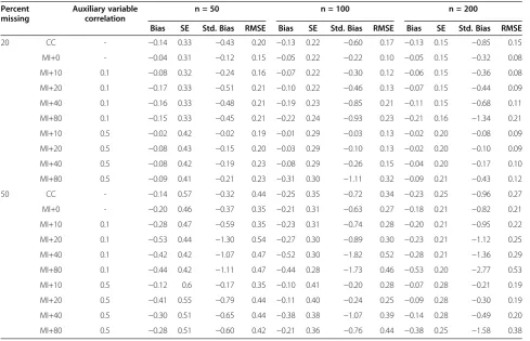
Table 2 displays a similar simulation, but an MAR(X) condition was realized. The basic patterns are similar to Table 1. MI generally performed better than CC, bias Table 2 Results of the simulations on linear regressions, MAR(X)
Percent missing
Auxiliary variable correlation
n = 50 n = 100 n = 200
Bias SE Std. Bias RMSE Bias SE Std. Bias RMSE Bias SE Std. Bias RMSE
20 CC - −0.14 0.33 −0.43 0.20 −0.13 0.22 −0.60 0.17 −0.13 0.15 −0.85 0.15
MI+0 - −0.04 0.31 −0.12 0.15 −0.05 0.22 −0.22 0.10 −0.05 0.15 −0.32 0.08
MI+10 0.1 −0.08 0.32 −0.24 0.16 −0.07 0.22 −0.30 0.12 −0.06 0.15 −0.36 0.08
MI+20 0.1 −0.17 0.33 −0.51 0.21 −0.10 0.22 −0.46 0.13 −0.07 0.15 −0.44 0.09
MI+40 0.1 −0.16 0.33 −0.48 0.21 −0.19 0.23 −0.85 0.21 −0.11 0.15 −0.68 0.11
MI+80 0.1 −0.15 0.33 −0.45 0.21 −0.22 0.24 −0.93 0.23 −0.21 0.16 −1.34 0.21
MI+10 0.5 −0.02 0.42 −0.02 0.19 −0.01 0.29 −0.03 0.13 −0.02 0.20 −0.08 0.09
MI+20 0.5 −0.08 0.43 −0.15 0.20 −0.03 0.29 −0.10 0.13 −0.02 0.20 −0.10 0.09
MI+40 0.5 −0.08 0.42 −0.19 0.23 −0.08 0.29 −0.26 0.15 −0.04 0.20 −0.17 0.10
MI+80 0.5 −0.09 0.41 −0.21 0.23 −0.31 0.30 −1.11 0.32 −0.09 0.21 −0.43 0.12
50 CC - −0.14 0.57 −0.32 0.44 −0.25 0.35 −0.72 0.34 −0.23 0.25 −0.96 0.27
MI+0 - −0.20 0.46 −0.37 0.35 −0.21 0.31 −0.63 0.27 −0.18 0.21 −0.82 0.21
MI+10 0.1 −0.28 0.47 −0.59 0.35 −0.23 0.31 −0.74 0.28 −0.20 0.21 −0.95 0.22
MI+20 0.1 −0.53 0.44 −1.30 0.54 −0.27 0.30 −0.89 0.30 −0.23 0.21 −1.12 0.25
MI+40 0.1 −0.42 0.42 −1.07 0.47 −0.52 0.30 −1.82 0.52 −0.28 0.21 −1.36 0.29
MI+80 0.1 −0.44 0.42 −1.11 0.47 −0.44 0.28 −1.73 0.46 −0.53 0.20 −2.77 0.53
MI+10 0.5 −0.12 0.6 −0.17 0.35 −0.10 0.41 −0.20 0.28 −0.07 0.28 −0.21 0.19
MI+20 0.5 −0.41 0.55 −0.79 0.44 −0.11 0.40 −0.24 0.25 −0.09 0.28 −0.30 0.19
MI+40 0.5 −0.30 0.51 −0.65 0.44 −0.38 0.38 −1.07 0.39 −0.14 0.28 −0.49 0.20
and SE tended to increase with the number of auxiliary variables, the same holds true for the RMSE. However, there is one difference to MAR(Y): the inclusion of ten auxiliary variables with r =.5 was helpful in all sample
sizes, 20 variables with n≥100, and 40 variables with
n = 200. Including more variables caused a downward bias of coefficients and precision decreased as was observed under MAR(Y). For auxiliary variables with low correlations, no such effect was observed.
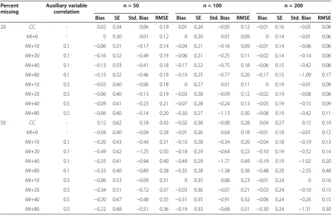
Table 3 displays a simulation where an MCAR condi-tion was realized. The basic patterns are different from Tables 1 and 2. Naturally, there was no bias under CC, so MI could not perform better than CC bias. Also, no benefit from including auxiliary variables could be observed regarding precision. However, including few auxiliary variables did not cause damage: ten auxiliary
variables did not introduce bias for n ≥ 100 for 20%
missing data, and for n = 200 also for 50% missing data–precision was only slightly worse then. Similar to the two MAR conditions, including too many auxiliary variables caused a downward bias of coefficients and a loss of precision.
A subset of simulations was replicated using different algorithms and programs. Some of the simulations were repeated using two different joint modelling algorithms,
Norm [23,32] and Amelia II [33]. Results were basically the same as those presented here, except that in small samples, the curves were less smooth when compared with the MICE algorithm. A similar result was reported by Taylor and Zhou [34]. Both programs, Amelia and Norm, broke down when the number of auxiliary vari-ables and the missing rate was high and the sample size low. For example, in samples of n = 100 and 20% miss-ing data, not more than about 40 auxiliary variables could be included. Three other programs based on the
MICE algorithm, STATA’s V12 [23], ICE [35] and
STA-TA’s“MI”[23] utilizing“chained (pmm)” and SPSS [36], basically led to the same results as R’s MICE. However, they also broke down when the number of auxiliary vari-ables (minus one) reached the number of cases with data. This is no disadvantage over MICE, given the results of the present simulation study. As this paper outlines, it makes no sense to reach a point where the number of variables is equal to the number of cases.
To explore if the present simulation results can be generalized to larger samples, we performed a simulation as defined above, having 50% missing data, MAR(Y), but 350 auxiliary variables, all r = .5, n = 1000. To reduce the computational time, only m = 5 imputed datasets were created and only 200 replications performed. Table 3 Results of the simulations on linear regressions, MCAR
Percent missing
Auxiliary variable correlation
n = 50 n = 100 n = 200
Bias SE Std. Bias RMSE Bias SE Std. Bias RMSE Bias SE Std. Bias RMSE
20 CC - 0.02 0.34 0.06 0.19 0.01 0.24 −0.05 0.12 −0.01 0.16 −0.05 0.08
MI+0 - 0 0.30 0.01 0.12 0 0.20 0.01 0.09 0 0.14 −0.01 0.06
MI+10 0.1 −0.06 0.31 −0.17 0.14 −0.04 0.21 −0.16 0.09 −0.01 0.14 −0.06 0.06
MI+20 0.1 −0.16 0.32 −0.49 0.19 −0.06 0.21 −0.25 0.11 −0.02 0.14 −0.14 0.06
MI+40 0.1 −0.13 0.33 −0.41 0.18 −0.17 0.22 −0.75 0.18 −0.06 0.15 −0.42 0.08
MI+80 0.1 −0.15 0.32 −0.46 0.19 −0.19 0.25 −0.77 0.20 −0.17 0.15 −1.09 0.17
MI+10 0.5 −0.03 0.40 −0.06 0.18 0 0.27 0.01 0.11 0 0.19 −0.01 0.08
MI+20 0.5 −0.06 0.40 −0.13 0.19 −0.03 0.28 −0.09 0.12 −0.02 0.19 −0.08 0.08
MI+40 0.5 −0.09 0.41 −0.23 0.21 −0.07 0.28 −0.24 0.13 −0.03 0.19 −0.15 0.09
MI+80 0.5 −0.06 0.40 −0.14 0.20 −0.30 0.27 −1.13 0.30 −0.08 0.19 −0.42 0.11
50 CC - 0.12 0.62 0.18 0.43 −0.02 0.38 −0.08 0.28 0.04 0.27 0.15 0.19
MI+0 - −0.04 0.40 −0.04 0.28 −0.01 0.26 0.04 0.18 −0.01 0.18 −0.01 0.12
MI+10 0.1 −0.20 0.43 −0.44 0.31 −0.10 0.28 −0.34 0.20 −0.04 0.18 −0.19 0.13
MI+20 0.1 −0.49 0.42 −1.25 0.50 −0.18 0.29 −0.64 0.22 −0.10 0.19 −0.52 0.14
MI+40 0.1 −0.35 0.41 −0.94 0.40 −0.49 0.29 −1.77 0.49 −0.19 0.19 −1.02 0.20
MI+80 0.1 −0.33 0.40 −0.89 0.38 −0.35 0.28 −1.38 0.38 −0.48 0.20 −2.55 0.48
MI+10 0.5 −0.06 0.53 −0.09 0.31 0 0.35 0.06 0.23 −0.01 0.24 0 0.16
MI+20 0.5 −0.34 0.51 −0.72 0.37 −0.03 0.36 −0.07 0.21 −0.03 0.24 −0.10 0.15
MI+40 0.5 −0.20 0.47 −0.48 0.35 −0.31 0.35 −0.91 0.32 −0.06 0.24 −0.26 0.15
Figure 1Regression coefficient b1in simulations with varying amounts of missing data, moderately correlated auxiliary variables
Results show a strong downward bias under MI+350
(bias = −.53, SE = .26, std. bias = −2.04, RMSE =
.54), even somewhat worse than under CC (bias =−.37,
SE = .25, std. bias = −1.48, RMSE = .39), compared to
MI+0 (bias = −.01, SE = .34, std. bias =−.03, RMSE =
.17).
Marshall et al. [27] compared various algorithms
(among them MICE and various joint modelling algo-rithms) in a simulation with eight predictors in a logistic regression with n=1000 subjects and did not find large differences. We would draw the conclusion that (1) the present effects of auxiliary variables were not the result of a specific program and that (2) in small samples, the MICE algorithm seems to perform better. However, in
large samples, one of the –usually much faster – joint
modelling algorithms would probably be preferable.
Example
In addition to the simulations, an example utilizing real data is provided. The data for this example is taken from an online survey, which was conducted in 2008 [37] in order to cross-validate a questionnaire, the SCL-27-plus. It is used to screen for symptoms of depression, agora-phobia, social anxiety, pain and vegetative symptoms. Questionnaires on quality of life [38] and parent–child relationships were also included [39]. For the present ex-ample, a score based on 8 items from the physical func-tioning scale of the quality of life (QOL) instrument was chosen as the response, and the pain score (six items) of the SCL-27-plus as a predictor (PAIN). In total, 48 add-itional items were used as auxiliary variables. Out of 500 cases, 100 were randomly chosen for this example. None of the cases had any missing data in QOL, PAIN or any auxiliary variable.
For the example, we conducted a simple regression analysis. The unstandardized b-coefficient for PAIN on
QOL was −1.97 with a standard error of 0.71 and a
t-value of −2.76 in the 100 cases with complete data. As
in the simulations, successively increasing numbers of observations (5%, 10%. . . 50% from all 40 items except the 8 for QOL were deleted using a 50% MAR(Y) and
50% MCAR mechanism – the higher the QOL, the
higher the probability the items were missing. After each step, two multiple imputations were performed and the impact on the following regression analysis examined. The first multiple imputation only used QOL and the six items of the score for PAIN for its imputation model (MI+0), the second used all other available variables as auxiliary variables for its imputation model (MI+48). The bivariate correlations between the variables were .23 on average, with the lowest being close to 0, and the highest .82. Program settings were identical compared to the simulated data.
When 5% of the observations were deleted, whether auxiliary variables were included or not made no visible difference. Both showed negligible bias with standard biases of−0.01 and 0.03, as compared to the value over the complete data. When the proportion of missing data rose, using no auxiliary variables for the imputation model did not increase bias. When 50% of the observa-tions were deleted and substituted, the relative bias was still less than 5% and the standard bias was only slightly increased to −0.08. Utilizing the 48 auxiliary variables introduced considerable bias with higher proportions of missing data. With 50% of the data missing, the standar-dized bias reached 0.99 and the mean b-coefficient was clearly biased towards zero.
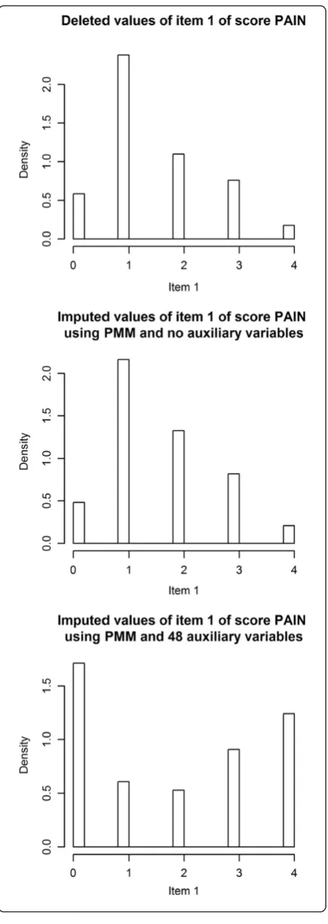
Figure 2 examined what happened when too many auxiliary variables were in the imputation model. The first item of the PAIN score is used for demonstration. The top figure shows the distribution of answers from 50 remaining cases when the other 50 were deleted. Be-cause the missing mechanism is partly MAR, the first distribution is not an approximation for the distribution of the complete data, but skewed. The second graph shows the distribution of the values that were imputed using no auxiliary variables. Virtually no difference from the first graph can be observed. The third graph shows the distribution of imputed values using all 48 auxiliary variables. It clearly deviates from the original data, with a much broader distribution.
Discussion
The results of the present simulation study can be sum-marized very briefly: In MI, inclusion of some auxiliary variables may help, too many can be harmful. Under MCAR, the inclusion of auxiliary variables was worthless and under MAR(Y), advantages were limited. The best results here were observed under the MAR(X) condition, where a reduction of bias plus an increase of precision could be reached by including a few auxiliary variables. Further, few auxiliary variables did not cause harm within the simulations realized here. The reason why too many variables introduce bias is probably that regression models become unstable when the ratio of cases to vari-ables gets low due to over-parameterization of the im-putation model. Standard textbooks usually recommend having at least ten cases per variable in regression mod-els. From the present simulations, we derived a prelimin-ary rule of thumb that is somewhat below the lower
limit of such recommendations–not to include a larger
rather than fewer auxiliary variables. These other recom-mendations should by no means be discredited by our simulation, they are correct - we merely want to show that the number of auxiliary variables that are included has an upper limit. We assume that the authors of these
recommendations consider it obvious that
over-parameterization needs to be avoided and therefore did not focus on it.
One of the main sources cited in these recommenda-tions is the simulation performed by Collins et al.[13]. We found five main differences between the Collins et al.simulations and ours.
(1) There were no missing values in our response; Collinset al.[13] observed the best effects of including auxiliary variables when the missing data were in the response. Hence, we included missing data in our response but still could not attribute a positive effect to auxiliary variables.
(2) Our auxiliary variables had correlations of r=.1 and r=.5, Collinset al.[13] used one variable with a correlation of r=.4 or r=.9. We were able to replicate the results from Collinset al.when including one variable with a correlation of r=.9. However, we did not want to use such high correlations because they are not likely to be observed in clinical research. When we performed simulations with correlations of r=.7 and higher, a stronger positive effect of including a few auxiliary variables could be observed. Particularly with relatively small amounts of missing data, we observed higher precision, with the drawback that larger amounts of missing data introduced bias. This data is not shown here because it is not realistic to assume such high correlations in real data. This result is congruent with a simulation performed by Enders and Peugh [40] who included six auxiliary variables into a factor analysis on samples with missing data rates of up to 25%. In this study, factor loadings were .60 - .70, and the correlations of the auxiliary variables were all r=.3. No substantial benefit from the auxiliary variables was observed. (3) Collinset al.had no missing data in the auxiliary variables themselves. Hence, we also performed a simulation where only the X’s had missing data. Results were very similar to the ones obtained by correlations of r=.7,i.e.a slightly positive effect of including a few auxiliary variables was observed. With relatively small amounts of missing data, a
higher precision was achieved, but again, with larger amounts of missing data, some bias occurred. (4) A further difference between our study and the
simulations performed by Collinset al.[13] was that in the latter, the auxiliary variable Z was associated with the likelihood for Y to be missing,i.e.an MNAR condition was introduced when the auxiliary variable was omitted. Hence, we performed a similar simulation, but in ours the value of Z was associated with the likelihood of X1andX2being missing. As a result, no positive effect of including this variable Z could be observed.
(5) Collinset al.[13] did not focus solely on a regression coefficient as we did here, but also examined means, standard deviations and
correlations. They observed stronger effects of the auxiliary variables on means and standard deviations than on regression coefficients.
From this, we can conclude that in estimating a linear
regression coefficient, (1) it doesn’t matter whether
missing values are in the explanatory variables only or also in the response, (2) inclusion of auxiliary variables is most helpful when the correlations to the X’s and Y are high (i.e.r≥|.5|), (3) auxiliary variables without missing data perform a little better than those that have missing data themselves, (4) a variable that explains the mechan-ism leading to missing data in the predictors need not necessarily be included in the imputation model and (5) regression coefficients are less sensitive to bias than means and standard deviations. Conclusion (4) in par-ticular came as a surprise to us, because it partially con-tradicts the intuitively appealing and well-accepted recommendation to keep the data MAR [14]. Further re-search is necessary to explore under which conditions it is beneficial to include a variable to keep the data MAR or whether including such a variable is disadvantageous. Conclusion (2) is similar to one provided by Enders [15], who has suggested that correlations greater than ± .40 are generally helpful.
A noteworthy effect was the drastic breakdown of the regression coefficient when too many variables were included, as displayed in Figures 1e and f. Therefore, we analyzed the distribution of the imputed values for Figure 1f when only 4% of the cases were missing (4 missing values × 20 imputed datasets × 1000 replica-tions = 80,000 data points). It turned out that there was an extreme variation in the imputed values–the standard deviation was 8 under this condition, instead of 1 as it was in the“observed”values. We repeated this analysis in our real data example with a higher percentage of miss-ing data and obtained the same result. An almost normal distribution of complete data changed to a U-shape by imputation with too many auxiliary variables.
In principle, this simulation study confirmed the ob-servation that under realistic conditions, a small amount of missing data (e.g.<5%) usually does not lead to severe bias or relevant loss in precision regardless which method of dealing with missing data is applied [27], in longitudinal studies, even larger missing rates can be tolerable [41]. However, when missing rates become higher and too many auxiliary variables are included in the imputation model, the regression coefficient can becomes seriously biased downward and imprecise (Figure 1e and f ). If multiple imputations are used at a ratio close to 1:1 of variables and cases, i.e. the point where chained equation programs often break down, even with small rates of missing data (i.e.5-10%), coeffi-cients can be seriously biased.
With the present simulations, we have tried to create conditions that are typical for data analyses in medicine
and life sciences, i.e. small to moderate sample sizes,
small to moderate correlations among the variables and small to moderate amounts of missing data. For small numbers of auxiliary variables, we saw an almost linear increase in bias and a decrease in precision with growing rates of missing data (Figure 1). However, as a rule of thumb, we suggest restricting the number of auxiliary variables to not more than 1/3 of the cases with complete
data, i.e. all cases minus those with missing data [5].
As an example, with 100 cases and 40% missing data, 60 cases have complete data. Hence, no more than 60/3 = 20 variables should be used in the imputation model. This holds true for continuous variables, and will not dramatically change when a few explanatory binary variables are in the model. Binary responses or datasets consisting mainly of binary or categorical variables with more than two categories will need a higher variables/ cases ratio–a simulation study on this is currently being planned? Using fewer variables should not be problem-atic, while using more variables would cause the risk for a serious downward bias of the regression coefficients. This was tested for samples of n=50, 100, and 200 under MCAR and two MAR mechanisms, including auxiliary variables with low or moderate correlations, and missing rates of up to 64%. Within the limits studied here, sample
size does not indicate a strong deviation from a “not
more than 1/3”rule, higher correlation of auxiliary vari-ables are better under MAR conditions, and MAR(X) profits more form auxiliary variables than MAR(Y).
The result can be plausibly extrapolated for larger
samples–our simulation with n=1000 and 350 variables
Situations may exist in which a substitution of very large
amounts of missing data (e.g. 90%) makes sense. In our
simulations, it did not. Marshallet al.[26,27] warned that using a multiple imputation that works well with less than 50% missing data introduces bias in a Cox regression when 75% of the data were missing. We do not recom-mend applying our rule to proportions of missing data larger than 64% without performing further simulations.
What to do when many variables are utilized in an ana-lysis with a limited sample size? Or if a statistician wants to impute the missing data in a set to make it freely us-able for public–in this case, he cannot know which stat-istical methods will be applied later. In such situations, including more variables than three times the number of
cases with complete data may be desirable –even
with-out considering any auxiliary variables. Then the choice of a program that allows a restriction of the number of predictors for each variable for which imputations are to
be done is recommended–mostly this would be a MICE
algorithm. This helps to avoid over-parameterization. Different possibilities in the various programs exist. Some (e.g.R’s mice, STATA) offer convenient ways to de-fine which variables are used as predictors for imputa-tions of other variables, others currently would make it difficult to do so (e.g.SPSS). If, further, the dataset con-sists of items belonging to different sub scales of a ques-tionnaire for example, it would make sense to use this information and to impute each subscale separately. If such a structure is not present, one should try to maximize the squared multiple correlations“using as few auxiliary variables as possible”[15], p. 133. With STATA
[23], such a selection needs to be done manually, R’s
mice provides a tool that automatizes this task quickpred: [25,42]. The predictor matrix can be displayed to see the selected variables and modified if desired.
Simulation studies should always be read with care. (1) We have only studied linear regression coefficients here. Other statistical parameters may be influenced dif-ferently by auxiliary variables. For example, in simula-tions by Hoo [16], positive effects on bias through inclusion of auxiliary variables were seen in some stand-ard errors in a confirmatory factor analysis, though the factor loadings themselves were not affected. (2) The present simulations are restricted to continuous data. Analysis of categorical data will introduce additional challenges. In that case, it is not only to be expected that the ratio variables/number of cases with complete data would be smaller, but the number of events per variable [43,44] will probably also become a parameter of interest. (3) In our simulations, all variables were dis-tributed normally and relations were perfectly linear. Both are not likely to happen in real data. Deviations from normal distribution may have a negative effect on the MI process, which should be examined in further
studies [45]. Problems of including quadratic or
inter-action effects were examined by Seaman et al. [46] and
van Buuren [42]. (4) In large surveys where thousands of cases are collected, even large numbers of variables may become a problem. This was not examined in detail here due to the limitations of computational power. Creating Figure 1f, for example, required more than 200 hours of computing time on a 6 physical core PC opti-mized for these simulations, and estimate of 350 vari-ables and 1000 cases about 60 hours. (5) We have displayed the distributions of the beta-coefficient only. This was done because research often focuses on the analysis of associations between variables. Simple point estimates of prevalence or means seem to benefit more from the inclusion of auxiliary variables. (6) Our simula-tions display downward bias. This is not necessarily
al-ways the case. Knol et al. [47] created four scenarios
where down- and upward bias occurred under CC.
Whether such upward bias, i.e. overestimation of an
as-sociation, can also occur under a multiple imputation is unknown.
To summarize, we have learned from the present simulation that in a typical life science survey, the in-clusion of auxiliary variables is often of little use; too many auxiliary variables may even be disadvantageous. Unless the correlations are high, we recommend keep-ing the number of variables in the imputation model as low as possible; even variables that explain the
mechanism leading to missing data don’t necessarily
need to be included. In our initial example, we used a researcher with 100 subjects that had ten scales based on six items each plus some demographics. This re-searcher was considering whether it would make more sense to substitute missing data on the item or on the scale level. Based on this example, our recommendation would be to impute in sub-models and to carefully se-lect the variables, rather than using one imputation model for all data.
Conclusion
Inclusion of too many auxiliary variables can ser-iously bias estimates in regression. We suggest a rule of thumb: that the number of cases with complete data should be at least three times the number of
variables – otherwise, restricting the number of
pre-dictors becomes an option. This holds true for data-sets containing mainly continuous and some binary variables. Performing MI in data sets consisting pre-dominantly of categorical variables, maybe even with many categories, will be even more difficult in small and medium samples.
Competing interests
The authors declare that they have no competing interests.
Authors’contributions
JH planned the paper and took a lead in writing it. MH carried out the simulations. RL planned the paper and corrected many details. All authors read and approved the final manuscript.
Author details
1Medical Psychology and Medical Sociology, Clinic for Psychosomatic
Medicine and Psychotherapy, University of Mainz, Duesbergweg 6, Mainz 55128, Germany.2Social Psychology and Methods, University of Freiburg,
Engelberger Straße 41, Freiburg 79106, Germany.
Received: 5 July 2012 Accepted: 28 November 2012 Published: 5 December 2012
References
1. Little RJ, Rubin DB:Statistical analysis with missing data. New York: Wiley; 2002. 2. Rubin DB:Multiple imputations after 18 plus years.JASA1996,
91:473–489.
3. Mackinnon A:The use and reporting of multiple imputation in medical research - a review.J Intern Med2010,268:586–593.
4. Karahalios A, Baglietto L, Carlin JB, English DR, Simpson JA:A review of the reporting and handling of missing data in cohort studies with repeated assessment of exposure measures.BMC Med Res Methodol2012,12:96. 5. Rubin DB:Multiple imputation for nonresponse in surveys. New York: Wiley &
Sons; 1987.
6. Little RJ:Regression with missing X's: a review.J Am Stat Assoc1992,
87:1227–1237.
7. White IR, Carlin JB:Bias and efficiency of multiple imputation compared with complete-case analysis for missing covariate values.Stat Med2010,
29:2920–2931.
8. Ambler G, Omar RZ, Royston P:A comparison of imputation techniques for handling missing predictor values in a risk model with a binary outcome.Stat Methods Med Res2007,16:277–298.
9. Eisemann N, Waldmann A, Katalinic A:Imputation of missing values of tumour stage in population-based cancer registration.BMC Med Res Methodol2011,11:129–142.
10. Marti H, Carcaillon L, Chavance M:Multiple imputation for estimating hazard ratios and predictive abilities in case-cohort surveys.BMC Med Res Methodol2012,12:24.
11. Soullier N, de La Rochebrochard E, Bouyer J:Multiple imputation for estimation of an occurrence rate in cohorts with attrition and discrete follow-up time points: a simulation study.BMC Med Res Methodol2010,
10:79–86.
12. Schenker N, Borrud LG, Burt VL, Curtin LR, Flegal KM, Hughes J, Johnson CL, Looker AC, Mirel L:Multiple imputation of missing dual-energy X-ray absorptiometry data in the national health and nutrition examination survey.Stat Med2011,30:260–276.
13. Collins LM, Schafer JL, Kam C-M:A comparison of inclusive and restrictive strategies in modern missing data procedures.Psychol Methods2001,
6:330–351.
14. Schafer JL, Graham JW:Missing data: our view of the state of the art.
Psychol Methods2002,7:147–177.
15. Enders CE:Applied missing data analysis. New York: Guilford; 2010. 16. Hoo JE:The effect of auxiliary variables and multiple imputation on
parameter estimation in confirmatory factor analysis.Educ Psychol Meas
2009,69:929–947.
17. White IR, Royston P, Wood AM:Multiple imputation using chained equations: Issues and guidance for practice.Stat Med2011,30:377–399. 18. Axen I, Bodin L, Kongsted A, Wedderkopp N, Jensen I, Bergstrom G:
Analyzing repeated data collected by mobile phones and frequent text messages. An example of low back pain measured weekly for 18 weeks.
BMC Med Res Methodol2012,12:105.
19. Cohen J:Statistical power analysis for behavioural sciences. Hillsdale, NY: Lawrence Erlbaum Associates; 1988.
20. Allison PD:Multiple imputation for missing data: a cautionary tale.Sociol Methods Res2000,28:301–309.
21. Horton NJ, Lipsitz JR:Multiple imputation in practice: Comparison of software pachages for regression models with missing variables.Am Stat
2001,55:244–254.
22. Graham JW, Olchowski AE, Gilreath TD:How many imputations are really needed? Some practical clarifications of multiple imputation theory.
Prev Sci2007,8:206–213.
23. StataCorp:Stata Statistical Software. Release 12. College Station, TX: StataCorp; 2011.
24. van Buuren S, Boshuizen HC, Knook DL:Multiple imputation of missing blood pressure covariates in survival analysis.Stat Med1999,
18:681–694.
25. Groothuis-Oudshoorn K, van Buuren S:Mice: multivariate imputation by chained equations in R.J Stat Software2011,45. http://www.jstatsoft.org/ v2045/i12003.
26. Marshall A, Altman DG, Holder RL:Comparison of imputation methods for handling missing covariate data when fitting a Cox proportional hazards model: a resampling study.BMC Med Res Methodol2010,
10:112.
27. Marshall A, Altman DG, Royston P, Holder RL:Comparison of techniques for handling missing covariate data within prognostic modelling studies: a simulation study.BMC Med Res Methodol2010,10:7.
28. Lee KJD, Carlin JBP:Recovery of information from multiple imputation: a simulation study.Emerg Themes Epidemiol2012,9:3. http://www.ete-online. com/content/pdf/1742-7622-1749-1743.pdf.
29. R Development Core Team:R: a language and environment for statistical computing. InBook R: a language and environment for statistical computing. City: R Foundation for Statistical Computing; 2011.
30. Becker RA:The new S language. Cole: Wadsworth & Brooks; 1988. 31. Eddelbuettel D:Random: an R package for true random numbers. 2006.
http://cranr-projectorg/web/packages/random/vignettes/random-intropdf. 32. Schafer JL:Analysis of incomplete multivariate data. New York: CRC Press; 1997. 33. Honaker J, King G:What to do about missing values in time serious cross
section data.American Journal of Political Science2010,2:561–581. 34. Taylor LM, Zhou XH:Multiple imputation methods for treatment
noncompliance and nonresponse in randomized clinical trials.Biometrics
2009,65:88–95.
35. ice: a program for multiple imputation: http://www.ats.ucla.edu/stat/stata/ library/ice.html.
36. SPSS Inc:SPSS V20. Chicago, IL: 2012.
37. Hardt J:The symptom-check-list-27-plus (SCL-27-plus): a modern conceptualization of a traditional screening instrument.German Medical Science - Psychosoc Med2008,5. http://www.egms.de/en/journals/psm/ 2008-2005/psm000053.shtml.
38. Hardt J, Stark H:Der Stark QoL- ein etwas anderer Fragebogen zur Lebensqualität. Poster zur 60. Arbeitstagungstagung der DKPM und 17. Jahrestagung der DGPM, Mainz, 18.-21. März.Psychol Med2009,20.
39. Hardt J, Dragan M, Kappis B:A short screening instrument for mental health problems: The Symptom Checklist-27 (SCL-27) in Poland and Germany.Int J Psychiatry Clin Pract2011,15:42–49.
40. Enders CK, Peugh JL:Using an EM covariance matrix to estimate structural equation models with missing data: choosing an adjusted sample size to improve the accuracy of inferences.Structural Equation Modeling2004,11:1–19.
41. Ranstam J, Turkiewicz A, Boonen S, Van Meirhaeghe J, Bastian L, Wardlaw D:
Alternative analyses for handling incomplete follow-up in the intention-to-treat analysis: the randomized controlled trial of balloon kyphoplastyversusnon-surgical care for vertebral compression fracture (FREE).BMC Med Res Methodol2012,12:35–47.
42. van Buuren S:Flexible imputation of missing data. Boca Raton: CRC Press (Chapman & Hall); 2012.
43. Peduzzi P, Concato J, Kemper E, Holford TR, Feinstein AR:A simulation study of the number of events per variable in logistic regression analsis.
J Clin Epidemiol1996,49:1373–1379.
44. Courvoisier DS, Combescure C, Agoritsas T, Gayet-Ageron A, Perneger TV:
Performance of logistic regression modeling: beyond the number of events per variable, the role of data structure.J Clin Epidemiol2011,
64:993–1000.
45. Yucel RM, Demirtas H:Impact of non-normal random effects on inference by multiple imputation: a simulation assessment.Comput Stat Data An
46. Seaman SR, Bartlett JW, White IR:Multiple imputation of missing covariates with non-linear effects and interactions: an evaluation of statistical methods.BMC Med Res Methodol2012,12:46.
47. Knol MJ, Janssen KJ, Donders AR, Egberts AC, Heerdink ER, Grobbee DE, Moons KG, Geerlings MI:Unpredictable bias when using the missing indicator method or complete case analysis for missing confounder values: an empirical example.J Clin Epidemiol2010,63:728–736.
doi:10.1186/1471-2288-12-184
Cite this article as:Hardtet al.:Auxiliary variables in multiple imputation in regression with missing X: a warning against including too many in small sample research.BMC Medical Research Methodology201212:184.
Submit your next manuscript to BioMed Central and take full advantage of:
• Convenient online submission
• Thorough peer review
• No space constraints or color figure charges
• Immediate publication on acceptance
• Inclusion in PubMed, CAS, Scopus and Google Scholar
• Research which is freely available for redistribution