A DESCENT PRP CONJUGATE GRADIENT METHOD FOR UNCONSTRAINED OPTIMIZATION
H. NOSRATIPOUR1, K. AMINI1, §
Abstract. It is well known that the sufficient descent condition is very important to the global convergence of the nonlinear conjugate gradient methods. Also, the direction generated by a conjugate gradient method may not be a descent direction. In this paper, we propose a new Armijo-type line search algorithm such that the direction generated by the PRP conjugate gradient method has the sufficient descent property and ensures the global convergence of the PRP conjugate gradient method for the unconstrained minimization of nonconvex differentiable functions. We also present some numerical results to show the efficiency of the proposed method.The results show the efficiency of the proposed method in the sense of the performance profile introduced by Dolan and Mor´e.
Keywords: Unconstrained optimization, Armijo-type line search, Conjugate gradient method, sufficient descent, Global convergence.
AMS Subject Classification: 90C30, 65K05
1. Introduction
The nonlinear conjugate gradient (CG) method plays a very important role for solving the unconstrained optimization problem
minf(x), x∈Rn (1)
wheref :Rn→Ris continuously differentiable. CG methods are usually designed by the
iterative form
xk+1 =xk+αkdk, (2)
wherexk is the current iterate point,αk>0 is a steplength anddkis the search direction
defined by
dk=
−gk ifk= 0
−gk+βkdk−1 ifk≥1 (3)
1 Razi University, Faculty of Science, Department of Mathematics, Kermanshah, Iran.
e-mail: [email protected]; ORCID: https://orcid.org/0000-0001-8801-9301. e-mail: [email protected]; ORCID: https://orcid.org/0000-0002-9264-3091.
§ Manuscript received: May 13, 2017; accepted: October 10, 2017.
TWMS Journal of Applied and Engineering Mathematics, Vol.9, No.3 cI¸sık University, Depart-ment of Mathematics, 2019; all rights reserved.
whereβk∈Ris known as the conjugate gradient parameter. A lot of versions of conjugate
gradient methods, correspond to the selection procedure of parameters βk, are already
known. Some of these selections are given as follows.
βkF R = kgkk 2
kgk−1k2
, (4)
βkDY = kgkk 2 (gk−gk−1)Tdk−1
, (5)
βP RPk = g
T
k(gk−gk−1)
kgk−1k2
, (6)
βkHS = g
T
k(gk−gk−1) (gk−gk−1)Tdk−1
, (7)
where k.k denotes the Euclidian norm [8, 12, 11, 17, 2, 5]. Although these methods are equivalent when f is a strictly convex quadratic function and αk is computed by the
following exact line search rule, i.e.
f(xk+αkdk) = min
α>0f(xk+αdk), (8)
but their behaviors for general objective functions may be far different. Their convergence properties have been studied by many authors, including [8, 12, 11, 17, 2, 5].
The global convergence of the PRP method is established whenf is strongly convex and the line search is exact [13]. Powell [15] has proved that for a general nonlinear function, the PRP is globally convergent if
(1) the stepsizexk+1−xk approaches zero,
(2) the line search is exact,
(3) the Lipschitz Assumption ofg holds.
In 1984, by using of a 3 dimensional example, Powell [14] showed that even withαk
ob-tained by an exact line search, the PRP method can cycle infinitely without approaching to a stationary point. Hence, this assumption that the stepsize tends to zero is needed for convergence. Under the assumption that the search direction is a descent direction, Yuan [20] has established the global convergence of the PRP method for strongly convex objec-tive functions along with the Wolfe line search. However, for the strong Wolfe line search, Dai [3] has introduced an example which shows that even when the objective function is strongly convex andσ∈(0,1) (the parameter of curvature condition) is sufficiently small, the PRP method may still fail by generating an ascent search direction.
In summary, the convergence of the PRP method for general nonlinear function is uncertain, Powell’s example shows that when the function is not strongly convex, the PRP method may not converge even with an exact line search. Based on insight gained from this example and to cope with possible convergence failure in the PRP algorithm, Powell [15] has suggested the following modification in the update parameter for the PRP method as
βkP RP+ = max{βkP RP,0}. (9) Gilbert and Nocedal [9] have shown that this choice guarantees the global convergence of the PRP+ algorithm. However, for the unconstrained minimization of strongly convex (nonquadratic) functions with exact line searches, Gilbert and Nocedal showed thatβkP RP
can be negative when the PRP method is convergent. This indicates that the choiceβkP RP+
functions and possibly decreases the rapid convergence of algorithm.
Another important approach for rectifying the convergence failure in the PRP algorithm is to retain the PRP update formula and modify the line search. In this regard, Grippo and Lucidi [10] by modifying Leone et al.’s line search [6] proposed an new line search as follows.
Given constants τ >0, σ ∈(0,1), δ >0 and 0< c1 <1< c2, their line search aims to find
αk= max{σjτ
|gTkdk|
kdkk2
; j = 0,1,· · ·}, (10)
such thatxk+1 =xk+αkdk withdk+1=−gk+1+βkP RP+1 dk satisfies
f(xk+1)≤f(xk)−δα2kkdkk2, (11)
and
−c2kgk+1k2 ≤gkT+1dk+1 ≤ −c1kgk+1k2. (12) Grippo and Lucidi [10] have proved the global convergence of the PRP conjugate gradient method equipped the line search rule (10)-(12) for the unconstrained minimization of nonconvex differentiable functions.
Dai [4] also has proposed a new line search for nonlinear conjugate gradient methods as follows.
Given λ∈ (0,1), δ ∈(0,1) and c1 ∈(0,1), determine the smallest integer m ≥0 such that if one defines
αk=λm, (13)
then
f(xk+αkdk)≤fk+δαkgkTdk, (14)
06=gTk+1dk+1≤ −c1kdk+1k2. (15) The global convergence of the PRP conjugate gradient method with this line search rule has been proved in [4].
The PRP method generally performs better than the other conjugate gradient methods in practice. However, it is not generally a descent method when Armijo-type line search is used, thus [10] and [4] for satisfying sufficient descent property added the extra relation (12) and (15) to Armijo-type line search, respectively. These strategies are valuable from the theoretical viewpoint.
It has been proved that these line search approaches are well defined and have the advantage that they can guarantee the global convergence of the original PRP method. However similarly to the strong Wolfe line search, they are computationally expensive. More precisely, to calculate a steplength to satisfy in the second condition any of these strategies (i.e., the inequalities (12) and (15)), it may be necessary to computegk+1 and
dk+1several times in each iteration. Hence, it is clear that the above mentioned line search rules are more computationally expensive.
The purpose of this paper is to overcome this drawback. To this end, using an estimated local Lipschitz constant of the derivative of objective function and choosing an adequate initial steplength sk, we modify and improve the two line search strategies proposed in
[4, 10] for computing a suitable steplength αk at each iteration by omitting the second
inequalities (12) and (15). We prove that, under some mild conditions, the PRP method along with the new line search rules generate search directions that satisfy the sufficient descent condition. Also, the PRP method is proved to be strong globally convergent.
The paper is organized as follows. In §2, we present a new Armijo-type line search. In
of the adaptive initial steplength sk and the new line search rules, we reported some
numerical results.
Notation. Throughout this paperg(x) =∇f(x) denotes the gradient of f(x). We write
k.k for the Euclidean norm of a vector. Furthermore, For all values, a subscript k means that this is the evaluation atxk or the value in thekth iteration, e.g., fk,gk.
2. New algorithm
In this section, we propose a modified Armijo-type line search that is used in con-junction with the PRP method. Its form is similar to that is given in relation (11) by Grippo and Lucidi but with different initial steplength sk which allows us to establish a
global convergence result. Throughout this paper, we consider the following assumptions in order to analyze the new algorithm:
(H1). The function f is continuously differentiable and bounded below on the level setL(x0) ={x∈Rn|f(x)≤f(x0)} .
(H2)The gradientg(x) of f(x) is Lipschitz continuous over an open convexS that con-tainsL(x0); i.e., there exists a positive constantL such that
kg(x)−g(y)k ≤Lkx−yk,
for allx, y∈S.
Considering the points listed in beginning of this section, we now present Algorithm 1 to describe the steps of the PRP method with a new Armijo-type line search as follows.
In the following, we assume an infinite sequence{xk}is generated, otherwise, Algorithm
1 stops at a stationary point of problem (1).
Lemma 2.1. Suppose that (H2) holds and Algorithm 1 generates an infinite sequence {xk}, then there exists c∈(0,1), such that
(c−2)kgkk2 ≤gkTdk≤ −ckgkk2. (16)
Proof. By induction, fork= 0,g0Td0 =−kg0k2, since 0< c <1, we have (c−2)kg0k2 ≤ −kg0k2 ≤ckg0k2,
so (16) holds. Fork≥1, from (3) and (6) we have
gTkdk=−kgkk2+βkP RPgTkdk−1. Using of hypothesis induction, we havegTk−1dk−1 <0 , then
|gTkdk+kgkk2|=|βkP RPgkTdk−1|
≤ kgkk
2|kg
k−gk−1k
kgk−1k2
kdk−1k
≤ Lαk−1kdk−1k
2
kgk−1k2
kgkk2
≤ Lsk−1kdk−1k
2
kgk−1k2
Algorithm 1: PRP method with an new Armijo-type line search
Input: x0∈Rn, constantsδ ∈(0,1), ρ∈(0,1), c∈(0,1), and a stoping tolerance >0;
Output: xb,fb; 1 begin
2 computef0 andg0;
3 k←0;
4 whilekgkk ≥do
5 computedk by (3) and (6);
6 setsk← 1−Lc
kgkk2
kdkk2;
7 α←sk;
8 bxk←xk+αdk;
9 whilef(xbk)> fk−α2|dkk2 do
10 α←ρα;
11 xbk←xk+αdk;
12 end
13 xk+1 ←xbk;fk+1 ←f(xbk);
14 computegk+1;
15 k←k+ 1;
16 end
17 xb ←xk;fb←fk; 18 end
So, by the definition ofsk, we have
|gkTdk+kgkk2| ≤(1−c)kgkk2
and
(c−2)kgkk2 ≤gTkdk≤ −ckgkk2.
Thus (16) holds and the proof is complete.
Lemma 2.2. Suppose that (H2) holds and Algorithm 1 generates an infinite sequence {xk}, then there exists c∈(0,1), such that
kdkk ≤(2−c)kgkk. (17)
Proof. Fork= 0, kd0k=kg0k, and so (17) holds. Fork≥1, from (3) and (6) we have
kdkk=k −gk+βkP RPdk−1k
≤ kgkk+
kgkkkgk−gk−1k
kgk−1k2
kdk−1k
≤(1 +Lαk−1kdk−1k 2
kgk−1k2
)kgkk
≤(1 +Lsk−1kdk−1k 2
kgk−1k2
)kgkk.
So, by the definition ofsk, we have
Thus (17) holds and the proof is complete.
Lemma 2.3. Suppose that (H1) and (H2) hold, then the line search (11) is well-defined.
Proof. By Taylor theorem, we can observe
f(xk+αdk) =fk+αgkTdk+O(α2kdkk2).
So, we deduce
lim
α→0+
fk−f(xk+αdk)−δα2kdkk2
α
= lim
α→0+
−αgkTdk−O(α2kdkk2)−δα2kdkk2
α
=−gTkdk>0.
Sinceα >0, it is concluded that there exists ´αk>0 such that
f(xk+αdk)≤fk−δα2kdkk2, ∀α∈[0,α´k].
Setting ˆαk = min(sk,α´k) yields
f(xk+αdk)≤fk−δα2kdkk2, ∀α∈[0,αˆk].
So, the new line search is well-defined and the proof is complete.
3. Convergence analysis
In this section, we prove the global convergence of Algorithm 1 under mild assump-tions.
Lemma 3.1. Suppose that (H1) and (H2) hold and Algorithm 1 generates an infinite sequence{xk}. then
η0 = inf
∀k≥0{αk}, (18)
is positive.
Proof. On the contrary, we suppose η0 = 0. So, there exists an infinite subset K ⊆
{0,1,2, ...}such that
lim
k∈K ,k→∞αk= 0. (19)
By the definition ofsk and (17), we have
sk ≥
1−c
L(2−c)2 >0. (20)
Thus, the sequence{sk}is positive and bounded from below. This along with (19) imply
that there is ´k such that
αk/ρ≤sk ∀k≥k and k´ ∈K.
On the other hand, from the line search rule (11), we observe that ˆα = αk/ρ doesn’t
satisfy (11), so
f(xk+ ˆαdk)> fk−δαˆ2kdkk2. (21)
This leads to
f(xk+ ˆαdk)−fk>−δαˆ2kdkk2. (22)
Using the mean value theorem on the left-hand side of the above inequality, there exists
θk∈(0,1) such that
so
−δαˆ2kdkk2<αgˆ (xk+ ˆαθkdk)Tdk.
Thus, we can deduce
−δαˆkdkk2 < gTkdk+ (g(xk+ ˆαθkdk)−gk)Tdk. (23)
By the Cauchy-Schwartz inequality and (23), we have
−δαˆkdkk2 < gTkdk+kg(xk+ ˆαθkdk)−gkkkdkk. (24)
Using of (H2) along withθk ∈(0,1) , we have
−δαˆkdkk2 < gTkdk+Lαθˆ kkdkk2 < gTkdk+Lαˆkdkk2. (25)
Thus, we obtain
ˆ
α≥ 1 L+δ
−gTkdk
kdkk2
. (26)
Sincedk is a descent direction, so we have
αk = ˆαρ≥
ρ L+δ
|gT kdk|
kdkk2
. (27)
It follows from (27), Lemma 2.1 and Lemma 2.2 that
αk≥
ρc
(L+δ)(2−c)2 >0 f or k≥k.´ (28) This contradicts (19). Therefore the proof is complete.
Theorem 3.1. Suppose that (H1) and (H2) hold and Algorithm 1 generates an infinite sequence{xk}. Then
lim
k→∞kgkk= 0. (29)
Proof. Cauchy-Schwartz inequality and Lemma 2.1 along with gTkdk≤0 imply that
kdkk ≥ckgkk. (30)
By Lemma 3.1, (11) and (30), we have
fk−fk+1≥δα2kkdkk2 ≥δη02c2kgkk2. (31)
This accompanied by assumption (H1) get
X
k≥0
kgkk2 <+∞.
Thus (29) is hold and the proof is complete.
4. Discussion
In Algorithm 1, we have proposed an Armijo-type line search rule equipped an adaptive initial steplength to be used in conjunction with the PRP method and established some convergence results. We note the proposed Armijo-type line search rule base on
f(xk+1)≤f(xk)−δα2kkdkk2, (32)
is also suitable for free-derivative methods. In comparison with the usual acceptance condition
the condition (32) enforces a greater reduction of f, for large values of αkkdkk, while it
becomes more tolerant when αkkdkk is small. In practical computations, to make the
steplengthαk easily accepted, it may be very useful to use the followingad hoc condition
f(xk+αkdk)≤fk+ max{δαkgkTdk,−γαk2kdkk2}, (34)
whereδ and γ are constants in (0, 1)[4]. In fact, in the right hand side of (34), the max term makes steplength to be more easily accepted than the acceptance conditions (32) and (33).
we wonder whether, when the condition (32) in Algorithm 1 is replaced to the condition (33) or the condition (34), the similar convergence results can be established. The answer is Yes, and it is interesting that the theoretical results obtained in previous Lemmas and Theorem 3.1 are still true. Moreover, if initial steplength in Algorithm 1 is replaced to
sk=ρk
|gkTdk|
kdkk2
, (35)
proposed in [10] withρk= 1−Lc, for allk, then the theoretical results obtained in previous
Lemmas and Theorem 3.1 are still true.
5. Numerical results
In this section, we report some computational performances of the new algorithm on a set including 75 unconstrained optimization test problems. The test problems and initial points have been selected from Andrei collection of unconstrained test functions [1]. We have performed our experiments in double precision arithmetic format in MATLAB
7.4 programming environment on a 2.54 GHz Intel single-core processor computer with 512 MB of RAM. Our results are reported for the following four PRP algorithms:
AN1: Algorithm 1;
AN2: Algorithm 1 with the acceptance condition (33);
Max: Algorithm 1 with the acceptance condition (34);
GL: Algorithm 1 with with initial steplengthsk computed by (35).
It is observed that L, the Lipschitz constant, plays an important role in the algorithm 1, butL is not generally known in practical computation. So, we need to estimate it at each iteration for using in the proposed line search. we can set a largeLkto guarantee the
global convergence. However, if Lk is very large then αk will be very small and will slow
the convergence rate of descent methods. On the other hand, very small values ofLkmay
fail to guarantee the global convergence. Thus, it is better to set an adequate estimation
Lkat each iteration. Recently, some approaches for estimatingLwere proposed in [18, 19].
For example, Shi and Guo [19] proposed an approximation for the Lipschitz constant in thekth iteration as follows.
Lk= max(L0,
kgk−gk−1k
kxk−xk−1k
), (36)
withL0 >0.
In all algorithms, we set δ = γ = 0.25, ρ = 0.9, c = 0.51 and L0 = 3. We also use (36) to estimate L for using in the proposed line search. All attempts to solve the test problems were limited to achieving a solution with
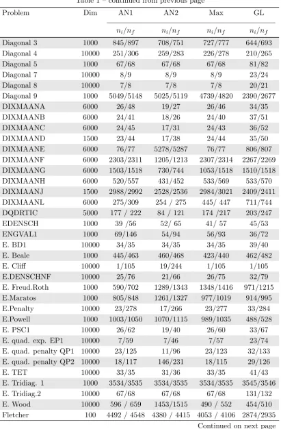
kgkk ≤10−6kg0k, (37) the numerical results are given in Table 1 which the columns have the following meanings:
Problem: The test problem name;
Dim: The dimension of the test problem;
ni: The total number of iterations;
nf: The total number of function evaluations.
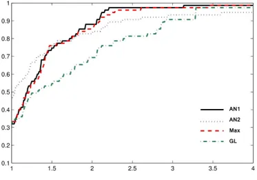
In the following, we offer some observations about the numerical results related to the total number of iterations from Table 1. First, we observe that the methods AN1, AN2 and Max that use the same initial steplength are superior than the method GL that uses another steplength. When comparing the methods AN1, AN2 and Max, we see that the methods AN2 and Max are faster than the methods AN1.
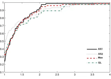
At the same time, for more comprehensive comparison between the methods, we adopt the performance profiles of Dolan and Mor´e [7] to to evaluate the number of iterations and the number of function evaluations. In Figures 1 and 2, the vertical axis gives the fraction
P of problems for which any given method is within a factor τ of the best performance. The left axis of the plot gives the percentage of the test problems for which a method needs least iterations. The right side of the plot gives the percentage of the test problems that are successfully solved by each of the methods. Clearly, the right side is a measure of an algorithms robustness.
Figure 2. Function evaluation performance profiles for the four algorithms
steplength in line search procedure and uses the usual Armijo line search , then it will not be globally convergent Thus, the new initial steplengthsk used in line search procedure is
effective in theory and practical .
Table 1: Numerical results.
Problem Dim AN1 AN2 Max GL
ni/nf ni/nf ni/nf ni/nf
Almost.P. Quad. 1000 827/888 734/784 705/764 990/1048
ARGLINB 1000 8/378 7/367 8/367 23/392
ARGLINC 1000 8 / 377 7 / 366 7 / 374 23/390 ARWHEAD 1000 124/203 294/361 205/282 221/298 BDQRTIC 1000 728/ 878 674/803 741/894 909/1141 BG2 100 584 /632 996/997 996/997 382/383 Broyden Tridiag. 10000 138/151 277/289 178/216 207/214 COSINE 10000 26/27 26/27 26/27/1 73/74 CUBE 1000 581/643 587/645 519/580 1168/1224 Diagonal 1 1000 546/574 546/574 546/574 376/423 Diagonal 2 100 4785/4786 4785/4786 4785/4786 4799/4800
Table 1 – continued from previous page
Problem Dim AN1 AN2 Max GL
ni/nf ni/nf ni/nf ni/nf
Diagonal 3 1000 845/897 708/751 727/777 644/693 Diagonal 4 10000 251/306 259/283 226/278 210/265 Diagonal 5 1000 67/68 67/68 67/68 81/82
Diagonal 7 10000 8/9 8/9 8/9 23/24
Diagonal 8 10000 7/8 7/8 7/8 20/21
Diagonal 9 1000 5049/5148 5025/5119 4739/4820 2390/2677 DIXMAANA 6000 26/48 19/27 26/46 34/35 DIXMAANB 6000 24/41 18/26 24/40 37/51 DIXMAANC 6000 24/45 17/31 24/43 36/52 DIXMAAND 1500 23/44 17/38 24/44 35/50 DIXMAANE 6000 76/77 5278/5287 76/77 806/807 DIXMAANF 6000 2303/2311 1205/1213 2307/2314 2267/2269 DIXMAANG 6000 1503/1518 730/744 1053/1518 1510/1518 DIXMAANH 6000 520/557 431/452 533/569 533/570 DIXMAANJ 1500 2988/2992 2528/2536 2984/3021 2409/2411 DIXMAANL 6000 275/309 254 / 275 445/ 447 711/744 DQDRTIC 5000 177 / 222 84 / 121 174 /217 203/247 EDENSCH 1000 39 /56 52/ 65 41/ 57 45/53 ENGVAL1 1000 69/146 54/94 56/93 36/72
E. BD1 10000 34/35 34/35 34/35 39/40
E. Beale 1000 445/463 460/468 423/440 462/482 E. Cliff 10000 1/105 19/244 1/105 1/105 E.DENSCHNF 10000 25/76 21/66 26/75 32/79 E. Freud.Roth 1000 590/702 1289/1343 1348/1416 971/1215 E.Maratos 1000 805/848 1261/1327 977/1019 914/995 E.Penalty 10000 23/278 17/266 23/277 33/284 E.Powell 1000 1003/1050 1070/1115 989/1035 488/528 E. PSC1 10000 26/62 19/40 26/60 33/67 E. quad. exp. EP1 10000 7/59 7/46 7/57 23/74 E. quad. penalty QP1 10000 23/125 11/96 23/123 32/133 E. quad. penalty QP2 10000 18/117 146/231 18/115 29/126
E. TET 10000 33/35 31/36 33/35 41/43
E. Tridiag. 1 1000 3534/3535 3534/3535 3534/3535 3545/3546 E. Tridiag.2 10000 67/68 67/68 67/68 131/132 E. Wood 10000 596 / 659 1453/1515 490 / 552 454/510 Fletcher 100 4492 / 4548 4380 / 4415 4053 / 4106 2874/2935
Table 1 – continued from previous page
Problem Dim AN1 AN2 Max GL
ni/nf ni/nf ni/nf ni/nf
Full Hessian FH1 1000 927/1108 1053/1224 899/1078 1433/2115 Full Hessian FH3 1000 7/90 7/81 7/88 23/105 G. PSC1 10000 376/408 592/620 322/353 375/401 G.Quartic 10000 51/58 101/121 97/103 28/29 G. Rosenbrock 100 8681/8758 8895/ 8939 8746 / 8820 7375/7488 G. Tridiag. 1 10000 55/56 55/56 55/56 42/43 G. Tridiag. 2 10000 157/166 215/231 157/166 73/81 HARKERP2 1000 297 / 444 208 / 324 238 / 383 170/317
HIMELH 10000 30/31 30/31 30/31 34/35
LIARWHD 1000 2763/2859 2162/2231 3362/3445 1848/2044 NONDIA 10000 8 / 157 7 / 125 8 / 155 23/172 NONDQUAR 10000 148/250 150/242 170/270 177/278 NONSCOMP 1000 712/750 45/73 708/744 750/785 Par.Per.Quad. 1000 46/121 57/124 46/119 54/127 Per.Quad.tic 1000 720 / 783 847/897 646 / 706 585/645 Per. quad. diag. 5000 109 / 194 67 / 135 122 / 204 152/236 Per.Tridia. quad. 5000 1292/1383 1615/1680 1449/1538 1233/1322 POWER 100 5372/5445 5204/5275 5420/5491 2432/2501 Quadratic QF1 1000 768/813 726/769 874/917 596/637 Quadratic QF2 1000 1167/1217 1167/1215 1165/1213 832/901 QUARTC 1000 2846/2847 2846/2847 2846/2847 7643/7644 Raydan 1 1000 758/798 783/810 805/842 783/812 Raydan 2 1000 58/59 58/59 58/59 72/73
SINCOS 10000 26/62 19/40 26/60 33/67
Staircase 1 1000 1463/1583 1399/1509 799/917 2278/2397 Staircase 2 1000 1871/1991 1077/1187 2203/2321 1044/1163 TRIDIA 1000 7112/7180 7404/7454 7256/7322 4155/4217 Vardim 10000 23/606 16/594 23/605 33/610
6. Conclusion
such that the direction generated by the PRP conjugate gradient method has sufficient descent property and ensures that the PRP conjugate gradient method AN1 is globally convergent for general functions under proper conditions. In addition algorithms AN2 and Max that use the new initial steplength are globally convergent and competitive with another. It is interesting to note that if AN2 method doesn’t use the new initial steplength in line search procedure and uses the usual Armijo line search, then it will not be globally convergent. Thus, the new initial steplengthsk used in the new line search procedure is
effective in theory and practical.
References
[1] Andrei, N., (2008), An Unconstrained Optimization Test Functions Collection, Advanced Modeling and Optimization, 10(1), 147–161.
[2] Dai, Y.H., (2001), New properties of a nonlinear conjugate gradient method, Numerische Mathematik, 89, 83–98.
[3] Dai, Y.H., (1997), Analysis of conjugate gradient methods. Ph.D. thesis, Institute of Computational Mathematics and Scientific/Engineering Computing, Chinese Academy of Sciences.
[4] Dai, Y.H., (2002), Conjugate gradient methods with Armijo-type line searches, Acta Mathematicae Applicatae Sinica (English Series), 18(1), 123–130.
[5] Dai, Y.H., Yuan, Y., (1996), Convergence properties of the Fletcher-Reeves method, IMA Journal of Numerical Analysis, 16, 155–164.
[6] De L.R., Gaudioso, M., Grippo, L., (1984), Stopping criteria for linesearch methods without derivatives, Mathematical Programming, 30, 285–300.
[7] Dolan, E., Mor´e, J.J., (2002), Benchmarking optimization software with performance profiles, Mathe-matical Programming, 91, 201–213.
[8] Fletcher, R. and Reeves, C., (1964), Function minimization by conjugate gradients, Computer Journal, 7, 149–154.
[9] Gilbert, J.C., Nocedal, J., (1992), Global convergence properties of conjugate gradient methods for optimization, SIAM Journal Optimization, 2, 21–42.
[10] Grippo, L., Lucidi, S., (1997), A globally convergent version of the Polak-Ribi´ere conjugate gradient method, Mathematical Programming, 78, 375–391.
[11] Hager, W.W., Zhang, H.C., (2005), A new conjugate gradient method with guaranteed descent and an efficient line search, SIAM Journal Optimization, 16, 170–192.
[12] Hestenes, M.R., Stiefel, E., (1952), Method of conjugate gradient for solving linear systems, Journal of research of the National Bureau of Standards, 49, 409–436.
[13] Polak, E., Ribi´ere, G., (1969), Note sur la convergence de directions conjug´ees. Rev, Francaise Informat Recherche Opertionelle, 3e Ann´ee, 16, 35–43.
[14] Powell, M.J.D., (1984), Nonconvex minimization calculations and the conjugate gradient method, Numerical Analysis, Dundee, 1983, Lecture Notes in Mathematics, Vol. 1066, Springer-Verlag, Berlin. 122–141.
[15] Powell, M.J.D., (1986), Convergence properties of algorithms for nonliniear optimization, SIAM Re-view, 26, 487–500.
[16] Powell, M.J.D., (1977), Restart procedures of the conjugate gradient method, Mathematical Program-ming, 2, 241–254.
[17] Shanno, D.F., (1978), On the convergence of a new conjugate gradient algorithm. SIAM Journal Numerical Analysis, 15, 1247–1257.
[18] Shi, Z.J., Shen, J., (2005), Step-size estimation for unconstrained optimization methods, Journal of Computational and Applied Mathematics, 24, 399–416.
[19] Shi, Z.J., Guo, J., (2009), A new family of conjugate gradient methods, Journal of Computational and Applied Mathematics, 224, 444–457.
Hadi Nosratipourwas born in Eslamabad-e Gharb, in Iran, in 1985. He obtained his PhD degree in Applied Mathematics in Operation Research area from Damghan University of Damghan, Iran in 2017. He obtained his MSc degree in Applied Mathe-matics in Operation Research area from Razi University of Kermanshah, Iran in 2011. His research interests include nonlinear optimization and optimal control.