A DYNAMICAL ANALYSIS OF THE VIRUS REPLICATION EPIDEMIC MODEL

A DYNAMICAL ANALYSIS OF THE VIRUS REPLICATION EPIDEMIC MODEL

I. KUSBEYZI AYBAR1,§

Abstract. In this article, the stability and the computational algebraic properties of a virus replication epidemic model is investigated. The model is represented by a three dimensional dynamical system with six parameters. The conditions for the existence of Hopf bifurcation in the system are given. Then, the model with the Beddington-DeAngelis functional response instead of the original nonlinear response function has been studied in order to understand the effect of the Beddington-DeAngelis functional response on the qualitative properties of the system. The stability of the systems at the singular points is investigated and the conditions for the systems to have the analytic first integrals and Hopf bifurcation are given. Finally, the results are illustrated by giving numerical examples.

Keywords: epidemic model, stability, analytic first integral, algebraic invariant, Hopf bifurcation.

AMS Subject Classification: 37G10, 65P30, 13A50

1. Introduction

An interesting epidemic model for the spread of disease is the Susceptible-Infected-Recovered (SIR) model which models the interaction between the susceptible (S) popu-lation which are susceptible to the virus, the infected (I) popupopu-lation which are infected by the virus and are infectious and the recovered (R) population which are recovered and gained immunity. In 1927, Kermack and McKendrick proposed a model to predict the number of people infected by a contagious illness, i.e. plague in a closed population over time in London during 1665-1666 and in Bombay in 1906 and another contagious illness,i.e. cholera in London 1865. This model stands as one of the first implementations of the SIR model and is referred to as the Kermack-McKendrick model[1].

Evolutionary relations between the parameters of the SIR model were investigated by Anderson and May by developing the models and fitting data[2, 3]. The periodicity and the stability properties in epidomiological models were studied by Hethcote et.al.[4, 5]. Smith showed that a period two bifurcation occurs for the SIR model when the contact rate parameter exceeds a threshold value[6]. In 1994, Kuznetsov and Piccardi studied the

1

Department of Computer Education and Instructional Technology, Faculty of Education, Yeditepe University, 34755, Atasehir, Istanbul, Turkey,

e-mail: [email protected]; ORCID: https://orcid.org/0000-0002-5531-0095.

§ Manuscript received: July 4, 2017; accepted: October 24, 2017.

TWMS Journal of Applied and Engineering Mathematics, Vol.9, No.2 cI¸sık University, Department of Mathematics, 2019; all rights reserved.

bifurcations of the periodic solutions of the SIR model with parameter portrait[7]. The stability and bifurcation properties of the endemic equilibria of a generalized SIR model were studied by Huang et.al.[8]. of In 1998, pulse vaccination was studied as an application of the SIR model and shown that the infected population converges to zero at a stable equilibrium point[9]. Lyapunov and global stability properties of the SIR model and its generalizations were investigated in 2002[10].

The SIR model and its generalizations have been investigated with delay[11, 12, 13, 14, 15, 16] or without delay[17, 18, 19, 20]. Beretta and Takeuchi studied the stability properties of an SIR epidemic model with time delays when the present force of infection depends on the number of the past infectives[21]. In this work they have shown that a disease free equilibrium state exists if there is no endemic equilibrium and if it exists, it is stable. In a more recent work, Ma et.al. gave the length of the time delay provided that the endemic equilibrium is global asymptotically stable by using the method by Freedman et.al.[22] to obtain the eventual lower bound[23]. Xu et.al. proposed a SIR epidemic model with nonlinear incidence and time delay and partially obtained the global stability of the endemic equilibrium for some given case[24]. Later, McCluskey enhanced this analysis to fully determine the global asymptotically stability of the endemic equilibrium whenever it exists[25]. Sun et. al. investigated the Hopf bifurcation for a virus infection model with an immune delay and two intracellular delays[26].

The SIR model is given by the following system[1]

dS dt =−

βIS N , dI

dt = βIS

N −γI, dR

dt =γI

(1)

whereS, I and R denote the numbers of the susceptible, the infected and the recovered population at time t, respectively. The parameter β denotes the infection rate and γ denotes the recovery rate. The parameters are assumed to be nonnegative. In the original SIR model no birth or death, i.e. no addition or removal of nodes from the population are assumed. However in real life, when the virus is fatal the node can not gain immunity and dies. Therefore, the node does not become susceptible again and has to be removed from the population. For this reason, the generalizations of the SIR model representing more realistic applications have to be taken into consideration.

model parasite-host interactions in predator-prey systems. The Beddington-DeAngelis functional response presents a more realistic consumption of predator over prey. Hence, it is interesting to study the Hopf bifurcation properties of the virus replication epidemic model with the Beddington-DeAngelis functional response.

In section 1, results on the stability of the equilibria and Hopf bifurcation analysis for the epidemic model with virus replication are presented and results are illustrated by giving a numerical example. In section 2, the same analyses is performed by replacing the simple nonlinear functional response with the Beddington-DeAngelis type nonlinear functional response in the model. We present our findings in comparison with the classic virus replication model.

2. The virus replication epidemic model

The epidemic model containing replication of the virus is given as[30, 31, 27] dx

dt =N −ax−bxz dy

dt =bxz−cy dz

dt =dy−ez.

(2)

Here,N is the constant population and ais the death rate of the uninfected population, bis the infection rate, c is the death rate of the infected population, dis the production rate and e is the decline rate of the recovered population which contains the free virus. All parameters are assumed to be positive to represent physical values.

Theorem 2.1. System (2)has at least one stable equilibrium.

Proof. The equilibria of system (2) are E1(N_a,0,0) and E2(_bdce,bdN−ace_bcd ,bdN_bce−ace) and the Jacobian matrix is

 

−a−bz 0 −bx

bz −c bx 0 d −e

 .

The eigenvalues of the Jacobian matrix at E1 are −a and −c+₂e ± √

a(4bdN+a(c−e)2₎

2a .

Hence,E1 is a stable equilibrium point.

Since we are not able to calculate the eigenvalues of the Jacobian at the equilibriumE2 by linear stability analysis, the Routh-Hurwitz criterion[32] is applied. The characteristic polynomial of the Jacobian matrix atE2 is

λ3+Aλ2+Bλ+C = 0 where

A= bdN

ce +c+e,

B = bdN(c+e) ce , C=bdN−ace.

analysis, i.e. choosing some parameters randomly, we look for conditions when the system has simpler geometric structure-admits an invariant surface or first integral and then study the obtained subsystem in more detail. Many systems with complex behavior such as a chemical reaction system[34], a two prey-one predator system[35], the May-Leonard model[36] and a gene model[37] have been investigated with the help of the method of algebraic invariants.

Remark 2.1. In system(2)Hopf bifurcation occurs atE1ifc=−eand4bdN+a(c−e)2 < 0. However, at E2 we can not find eigenvalues. Hence, it is possible to study Hopf bifurcation for the reduced system on the invariant plane, to find Hopf bifurcation for the three dimensional system.

We use the following approach to obtain the conditions in Theorem 2.3. In similar, we also obtain the conditions for the existence of the first integral of system (2) which are listed in Theorem 2.4. Let

f1(x1, ..., xn) = 0, ..., fk(x1, ..., .xn) = 0 (A)

be a polynomial system and letI =hf1, ..., fki ⊂k[x1, ..., xn] be the corresponding with

the implicit ordering of the variablesx1 > ... > xn.

Definition 2.1. Let I be an ideal in k[x1, ..., xn] and fix m ∈ {0, ..., n−1}. The m-th elimination ideal of I is the idealIm =I∩k[xm+1, ..., xn].

To eliminate x1, ..., xm(0≤m < n) from system (A) one can use the following theorem

(see [33] for the proof).

Theorem 2.2. (Elimination Theorem). Fix the lexicographic term order on the ring

k[x1, ..., xn] with x1 > x2 > ... > xn and let G be a Groebner basis for an ideal I of

k[x1, ..., xn]with respect to this order. Then for every m, 0≤m ≤n−1, the set Gm :=

G∩k[xm+1, ..., xn]is a Groebner basis for the m-th elimination ideal Im.

Using the Elimination Theorem we can determine the invariant algebraic surfaces of the form

L=a0+a1x+a2y+a3z+a4xy+a5xz+a6yz (3) of system (2).

Consider the system

˙

x=P(x, y, z), y˙ =Q(x, y, z), z˙=R(x, y, z). (4)

Let

D:= ∂

∂xP(x, y, z) + ∂

∂yQ(x, y, z) + ∂

∂zR(x, y, z)

be the vector field associated to (4) and letLbe a polynomial in the variablesx, y, z. The polynomialL defines an invariant algebraic surfaceL= 0 of system (4) if

DL=LK

for some polynomial K(x, y, z). The polynomial K is called the cofactor of L and has degree at most n−1, if the maximal degree of the polynomials P, Q and R is n. Since the polynomials on the right hand side of system (2) are of degree at most 2 we look for the cofactors of the formK =b0+b1x+b2y+b3zand the invariant algebraic surfaces of the form (3).

We perform all the computations in the computer algebra systems MATHEMATICA and SINGULAR[38].

Theorem 2.3. System (2) has an invariant surface of degree one or two if one of the following conditions is satisfied.

i. b= 0

ii. a−c= 0

iii. a−e= 0

iv. d=a±₂e =c±e₂ = 0

v. d=a±2e=c±2e= 0

vi. d=a±e=c±e= 0

vii. d=e= 0

Proof. Ifb= 0, system (2) has the invariant plane l1= 1− _Nax with the cofactor−a. If a=c, system (2) has the invariant plane l2= 1−_Ncx−_Ncy with the cofactor −c. Ifa=e, system (2) has the invariant planel3= 1−_Nex−_Ney+e(_dNe−c)zwith the cofactor

−e.

If d=a± e

2 =c±

e

2 = 0, the invariant plane of system (2) is l4= 1±

e

2Nx± e

2Ny with

the cofactor−e₂.

If d=c±2e=a±2e= 0, the invariant plane of system(2) isl5 = 1±2_βex±2_βey with the cofactor 2e.

If d= 0 and a =c = ∓e, system (2) has the invariant plane l6 = 1±_Nex± _Ney with the cofactore. Additionally system (2) has the invariant surface l7 = 1− _Nbxz with the cofactor−bzifd= 0 and a=c=−e.

If d=e= 0, system (2) has the invariant surfacel8 = 1−_Nax−_Nbxz with the cofactor

−c−e.

Remark 2.2. Squares of the invariant planes are invariant surfaces with the cofactors which are two times of the cofactors of those invariant planes. That is, if l1 = 1−_Nax is

an invariant plane of system (2) for b= 0 with the cofactor −a, then l0₁ = (1− a Nx)

2 _{is a}

trivial invariant surface of system (2)with the cofactor −2a.

Moreover, multiples of the invariant planes are invariant surfaces. For example, another trivial invariant surface of system (2) is l₂₃0 = 1−2_cebdx−bd₂(_cc2+_ee2)2y−

b(c2_−e2₎ 2c2_e z+

b2_d2

c2_e2x2+

b2_d2

c2_e2y2+2b 2_d2

c2_e2 xy+

b2_d(c−e)

c2_e2 xz+

b2_d(c−e)

c2_e2 yz with the cofactor−c−ewhen N bd−c₂(c+e) = a−c+₂e = 0 is satisfied, which is a combination of the invariant planesl2 and l3.

Theorem 2.4. System (2)has a first integral if one of the following conditions is satisfied. i. b=c= 0

ii. b=e= 0

iii. d=e= 0

iv. b=a+c= 0

v. b=a+e= 0

vi. b=c+e= 0

vii. d=a+e=c+e= 0

Proof. System has the first integrals Ψ1 = 1 +y and Ψ2= 1 +y+y2, ifb=c= 0. If b=e= 0, system (2) has the first integrals Ψ1 = 1 +y+ _dcz and Ψ2 = 1 +y+_dcz+ yz+₂d_cy2+₂c_dz2.

If d = e = 0, system (2) has the first integrals Ψ1 = 1 +z and Ψ2 = 1 +z+z2. If additionallyc=N = 0 is satisfied, system (2) has the additional integral Ψ3 = 1 + a_by+ xz+yz.

If b= 0 and a=−c, the first integral of system (2) is Ψ1 = 1 +y+_Ncxy. Ifb= 0 anda=−e, the first integral of system (2) is Ψ1 = 1+N_ey+N(

c−e)

de z+xy+ c−e

If b= 0 and c=−e, system (2) has the first integral Ψ1 = 1 +yz+−₂d_ey2.

If d= 0 and a=c=−e, system (2) has the first integral Ψ1 = 1 +N_ez+xz+yz.

Theorem 2.5. System (2)has stable Hopf bifurcation, if b >0,c >0, d <0 ande <−c.

Proof. We will look for Hopf bifurcation on the invariant plane of system (2). For this, we choose the invariant planel3= 1−_Nex−_Ney+e(_dNe−c)zwhich exists whena=e. By using the transformation

x= N

e +X−Y − c dZ+

e

dZ, y=Y, z =Z

we rewrite system (2) as

dX

dt =−eX, dY

dt =

be(e−c)Z2+bdeXZ−bdeY Z −cdeY +bdN Z

de ,

dZ

dt =dY −eZ.

(5)

According to the equilibria of system (5), there exists a possibility for a stable Hopf bifurcation to occur at the nontrivial equilibrium point (0,bdN_bcd−ce2,bdN−ce_bce 2). First, we move system (5) to this equilibrium point to have system

dX

dt =−eX, dY

dt = 1

cde(bce(e−c)Z

2_{+bcdeXZ−bcdeY Z+ (bd}2_{N −cde}2_)X + (cde2−c2de−bd2N)Y + (2c2e2−ce3−bcdN+bdeN)Z), dZ

dt =dY −eZ,

(6)

so that system (6) can have Hopf bifurcation at the origin if N = −c_bd2e. The reduced system onX= 0 is then

dY dt =

1

cde(bce(e−c)Z

2_{−bcdeY Z+ (cde}2_−c2_de−bd2_N)Y + (2c2e2−ce3−bcdN+bdeN)Z),

dZ

dt =dY −eZ

(7)

By calculating the first Lyapunov coefficient to check the stability of the Hopf bifurcation, we obtainα= _2(ce(c−eβcde_)+bdN),γ = β(c(c+_2dee)−e2) and

g1=−

βb2cd3

e(3c3_{(c+ 2ce) + 3(d}2_+e2₎2_−2ce(d2_{+ 3e}2_)−c2_(2d2_{+ 3e}2₎₎.

0.0 0.5 1.0 1.5 2.0 2.5 3.0 3.5

0.0 0.5 1.0 1.5

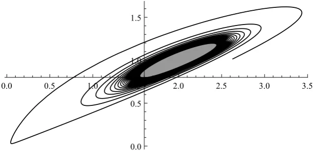
Figure 1. Stable Hopf bifurcation for system (8)

Example 2.1. Choosing the parameter values as{b, c, d, e}={1,1,−1,−2}, we have the two dimensional projection

dv dt =3w

2_−vw−v+ 99 100w, dw

dt =−v+ 2w

(8)

of system (2). System (8) goes under Hopf bifurcation at the equilibrium point (101₅₀,101₅₀)

with the eigenvalues ₂₀₀1 (−1±i√40399). The stable Hopf bifurcation bifurcating from this equilibrium point is shown in figure 1.

3. SIR model with the Beddington-DeAngelis functional response

Beddington[28] and DeAngelis[29] introduced the Beddington-DeAngelis functional re-sponse in 1975. The SIR model with Beddington-DeAngelis infection rate is given by

dx

dt =N −ax−

bxz 1 +αx+βz, dy

dt =

bxz

1 +αx+βz −cy, dz

dt =dy−ez

(9)

where all parameters are given as in section 1 except for the parametersα and β are the inhibitory effect parameters with respect to the Beddington-DeAngelis response function. We assume that all parameters are nonnegative to reflect physical values.

Theorem 3.1. System (9)has at least one stable equilibrium.

Proof. The Jacobian matrix of system (9) is

  

−a−₍₁₊bz(1+_αx+βz_βz)₎2 0 −

bx(1+αx) (1+αx+βz)2

bz(1+βz)

(1+αx+βz)2 −c

bx(1+αx) (1+αx+βz)2

0 d −e

  

E2(x2, y2, z2) =E2( ce+dβN d(b+aβ)−ceα,

bdN−ce(a+αN) c(d(b+aβ)−ceα),

d(bdN−ce(a+αN)) ce(d(b+aβ)−ceα) ).

The eigenvalues of the Jacobian matrix of system (9) at equilibrium E1 are −a and

−c+e

2 ±

√

(a+αN)(4bdN+(a+αN)(c−e)2₎

2(a+αN) . Hence E1 is a stable equilibrium considering a > 0 andN 6=−a_α and therefore one stable equilibrium of system (9) is guaranteed.

Now we give criteria for E2 to be a stable equilibrium of system (9). We obtain the characteristic equation of system (9) atE2 as

λ3+Aλ2+Bλ+C = 0 where

A= ce(bd(c+e) +aceα) + ((bd−ceα)

2_+bd2_(a+c+e)β)N

bd(ce+dβN) ,

B = (ac2e2((c+e)α−dβ) +abd2(c+e)βN

+ (bd−ceα)((c+e)(bd−ceα) +cdeβ)N)/(bd(ce+dβN)),

C= ce(d(b+aβ)−ceα)(bdN−ce(a+αN)) bd(ce+dβN) .

According to the Routh-Hurwitz criterion we conclude that if

(ac2e2((c+e)α−dβ) +abd2(c+e)βN + (bd−ceα) ((c+e)(bd−ceα) +cdeβ)N)(ce(bd(c+e) +aceα)

+((bd−ceα)2+bd2(a+c+e)β)N)

−bcde(ceα−d(b+aβ))(ce+dβN)(−bdN+ce(a+αN))>0

andA, B, C ≥0,x2 ≥0, y2≥0, z2≥0 andbd(ce+dβN)6= 0 are satisfied thenE2 is also a stable equilibrium of system (9).

Theorem 3.2. The invariant planes l1,...,7 given in corresponding cases of Theorem 2.3

are also invariant planes of system (9). Additionally system (9) has an invariant surface if one of the following cases are satisfied.

i. β=a−c+₂e =N(bd−ceα)−ce₂(c+e) = 0

ii. d=α=a−c−e= 0

iii. d=a−c+₂e =N α+ c+₂e = 0

iv. d=a−₂c =b+β(e−₂c) = 0

v. d=β(a−e)−b=a+N α= 0

vi. a−2c=cα+dβ=b+eβ = 0

vii. a−2e=eα+dβ=b+cβ= 0

viii. d=α=β =a+e= 0

Proof. Ifβ =a−c+e

2 =N(bd−ceα)−

ce

2(c+e) = 0, system (2) has the invariant surface l8 = 1 +

2(αce−bd) ce x+ (

αce−bd ce )

2_x2₋ 2bd(c+e)2(bd−αce) c2_e2_(αc2_{+ 4bd−2αce+αe}2₎y + 8bd(bd−αce)

2

c2_e2_(αc2_{+ 4bd−2αce+αe}2₎xy+

4bd(bd−αce)2

c2_e2_(αc2_{+ 4bd−2αce+αe}2₎y 2

− 2b(bd−αce)(c

2_−e2₎

c2_e(αc2_{+ 4bd−2αce+αe}2₎z+

4b(c−e)(bd−αce)2

c2_e2_(αc2_{+ 4bd−2αce+αe}2₎xz + 4b(c−e)(bd−αce)

2

c2_e2_(αc2_{+ 4bd−2αce+αe}2₎yz with the cofactor−c−e.

If d=α=a−c−e= 0, system (2) has the invariant surfacel9 = 1−c_N+ex−b(c_ce+e)z+

b(c+e)

eN xz+

(c+e)(b+βe)

eN yz with the cofactor −c−e.

If d=a−c+₂e =N α+ c+₂e = 0, system (2) has the invariant surface l10 = 1 + 2αx+ α2x2+2(_cbc_(c−e+be₎)z+_c−e4αbxz−2(−2αb+_c−eαβc−αβe)yz with the cofactor −c−e.

If d=a− c

2 =b+β(e−

c

2) = 0, system (2) has the invariant surface l11 = 1−

c Nx+ c2

4N2x2+

(−c2_−2αcN)

2αN2 y− bc 2

α(c2_−3ce+2e2_)Nz+ bc 2

α(c−2e)N2xz with the cofactor −c.

If d=β(a−e)−b=a+N α= 0, system (2) has the invariant surfacel12= 1 + 2αx+ α2x2+_e2₊₂αβN_αNz+ 2αβxz with the cofactor 2αN.

If a−2c=cα+dβ=b+eβ= 0, system (2) has the invariant surface

l13= 1 + 2βd αNx+

2αβd(dβ+eα)

α3_eN+α2_{βdN−αβde−2β}2_d2y+

2β2d2(2βd+αe)

N(α3_eN+α2_{βdN−αβde−2β}2_d2₎xy

+ β

2_d2_(2βd+αe)

N(α3_eN+α2_{βdN−αβde−2β}2_d2₎y

2₊ 2β3d2

α3_{eN +α}2_{βdN−αβde−2β}2_d2z

− 2β

3_d2_(2βd+αe)

αN(α3_eN+α2_{βdN −αβde−2β}2_d2₎xz with the cofactor 2βd_α .

If a−2e=eα+dβ=b+cβ= 0 system (2) has the invariant surface

l14= 1 + 2βd αNx+

2αβd(αc+βd)

α3_{cN +α}2_{βdN−αβcd−2β}2_d2y+

2β2d2(αc+ 2βd)

N(α3_cN+α2_{βdN −αβcd−2β}2_d2₎xy

+ β

2_d2_{(αc+ 2βd)}

N(α3_cN+α2_{βdN−αβcd−2β}2_d2₎y

2₊ 2αβc(αc+ 2βd)

α3_{cN +α}2_{βdN−αβcd−2β}2_d2z

+ 2β

2_{cd(αc+ 2βd)}

N(α3_cN+α2_{βdN−αβcd−2β}2_d2₎xz+

2β2d(α2c2+ 3αβcd+ 2β2d2) αN(α3_{cN +α}2_{βdN−αβcd−2β}2_d2₎yz

+ β

2_(αc+βd)2_{(αc+ 2βd)}

α2_N(α3_{cN +α}2_{βdN−αβcd−2β}2_d2₎z 2 with the cofactor 2βd_α .

If d=α=β =a+e= 0, system (2) has the invariant surface l15= 1−_Nbxz with the cofactor−bz.

Ifd=α=a−2e=c−e= 0, system (2) has the invariant surfacel16= 1−2_Nex−2_ebz+ 2b

Nxz+

2(b+βe)

N yz with the cofactor −2e.

Theorem 3.4. In system (9) Hopf bifurcation can occur on the invariant plane l2 of

system (9).

Proof. System (9) after the corresponding transformation with respect to the invariant planel1 = 1−_Nex−_Ney+e(_dNe−c)zwhich exists ifa=eis

dX

dt =−eX, dY

dt =(cdeαY

2_{+ (be(e−c))Z}2_{−cdeαXY +bdeXZ−(bde+ce(dβ−cα} +αe))Y Z−(cd(e+αN))Y +bdN Z)/(deαX−deαY −(eα(c−e)

−deβ)Z+d(e+αN)),

dZ

dt =dY −eZ

(10)

The Jacobian matrix of system (10) is  

−e 0 0

J21 J22 J23 0 d −e

 

where

J21=

bd2e2Z(1 +βZ)

(deαX−deαY + (deβ+eα(e−c))Z+d(e+αN))2, J22= (−α2cd2e2X2−α2cd2e2Y2−e2(β(b+βc)d2+α2c(c−e)2

+ 2αβcd(e−c))Z2+ 2α2cd2e2XY + (2αcde2(−βd+α(c−e)))XZ + 2αcde2(βd+α(e−c))Y Z−2αcd2e(e+αN)X+ 2αcd2e(e+αN)Y

−de(e((b+ 2βc)d+ 2αc(e−c)) + 2αcN(βd+α(e−c)))Z−cd2(e+αN)2) /(deαX−deαY + (deβ+eα(e−c))Z+d(e+αN))2,

J23= (bd2e2αX2+bd2e2αY2+be(eα(c(c−2e) +e2)−deβ(c+e))Z2

−2bd2e2αXY + 2bdeα(e(e−c))XZ+ 2bdeα(e(c−e))Y Z+bd2e(e+ 2αN)X

−bd2e(e+ 2αN)Y + 2bde(e−c)(e+αN)Z+bd2N(e+αN) /(deαX−deαY + (deβ+eα(e−c))Z+d(e+αN))2.

The equilibrium points of system (10) are F0(0,0,0) and F1(0,

ce(e+αN)−bdN c(ceα−d(b+eβ)),

d(ce(e+αN))−bdN) ce(ceα−d(b+eβ))) ). The eigenvalues of the Jacobian matrix atF0 are −eand

1

2(e+αN)(−(c+e)(e+αN)± p

(e+αN)(e(c−e)2_{+ (4bd+α(c−e)}2_)N)). We see that Hopf bifurcation can not occur at F0 for physical values of the parameters. However if we assume c = −e < 0 system (10) can go through Hopf bifurcation at F0 under one of the following set of conditions.

i. b <0,d >−α(c−e_4b )2 and N >−_4bde₊(c−e_α(c−e)2 ₎2,

ii. b >0,α= 0, d >0,N <−e(c−e_4bd)2 and henceN <0, iii. b >0,α >0,d >0,−e

α < N <−

e(c−e)2

iv. b >0,α <0, 0< d <−α(c−e_4b )2,−e

α < N <−

e(c−e)2

4bd+α(c−e)2 and henceN <0, v. b >0,α <0,d≥ −α(c−e_4b )2,N >−_αe and henceN <0,

vi. b >0,e >0,d <−α(c−e_4b )2,N >−_4bde₊(c−e_α(c−e)2₎2 and hence d <0. The eigenvalues of the Jacobian matrix at F1 are −eand

−1

2bd2_(ce+dβN)(d(bd

2_{N(b+β(c+e)) +bcde(c−2αβ) +αc}2_e2_(e+αβ))±√_∆) where

∆ = (d2(b4d4β2+c4e4α2(e+αβ)2−2b3d3β(c2e−deβ+cβ(dβ+ 2eα)) +b2d2(c3e2(c+ 4e) + 2c2eβ(dβ(c+e) +eα(2c+e)) + (d2β2(c−e)2 + 4cdeαβ(c−e) + 6c2e2α2)β2)−2bc2de2(e+αβ)(c2eα+dαβ2(c−e) + 2ceα2β−2dβ(ce+dβ2)).

Hopf bifurcation can occur at F1 if αce

b+βe < d < αce

b and

β = −bc

2_de−αc2_e3

b2_d2_+bβcd2_{−2bαcde+bβd}2_e+α2_c2_e2 <0 is satisfied.

We move system (10) to F1 to have system dx

dt =−ex, dy

dt =(αc

2_{de(bd−αce+βde)y}2_{−bc(c−e)e(bd−αce+βde)z}2_+αc2_de(αce

−d(b+βe))xy+bcde(bd−αce+βde)xz−ce(bd−αce+βde)

((b+βc)d+αc(e−c))yz+d(bd−αce)(bdN−ce(e+αN))x

−d(b2d2N +αc2e2(e+αN) +bcd(ce+βdN−e(e+ 2αN)))y + (b2d2(e−c)N +c2e2(βd+α(e−c))(e+αN) +bcde(2c(e+αN)

−e(e+ 2αN)))z)/(αcde(bd−αce+βde)x+αcde(αce−d(b+βe))y

+ce(bd−αce+βde)(βd+α(e−c))z+bd2(ce+βdN)), dz

dt =dy−ez

(11)

Then by introducingx= 0 into system (11) we have the following reduced system. dy

dt =(αc

2_{de(bd−αce+βde)y}2_{−bc(c−e)e(bd−αce+βde)z}2_+αc2_de(αce

−ce(bd−αce+βde)−d(b2d2N +αc2e2(e+αN) +bcd(ce+βdN−e(e+ 2αN)))y

+ (b2d2(e−c)N+c2e2(βd+α(e−c))(e+αN) +bcde(2c(e+αN)

−e(e+ 2αN)))z)/(αcde(αce−d(b+βe))y

+ce(bd−αce+βde)(βd+α(e−c))z+bd2(ce+βdN)), dz

dt =dy−ez

We see that system (2) can be reduced to two dimensions by using the transformation defined by the algebraic invariant plane as in system (1). So, Hopf bifurcation exists for system (2). However, it is not possible to calculate the first Lyapunov coefficient to find the stability of the Hopf bifurcation for system (2).

4. Conclusion

In this paper, we have investigated the stability and Hopf bifurcation properties of an original version and a generalized version with the Beddington-DeAngelis functional response epidemic model with virus replication. We have used the methods of computa-tional algebra, i.e. invariant planes where usual methods fail. Both models show Hopf bifurcation. We have found the parameter conditions for a stable Hopf bifurcation to oc-cur for the original virus replication model. However, it is not possible to find parametre conditions for the stability of the Hopf bifurcation of the virus replication model with the Beddington-DeAngelis functional response although the both models have the same invariant planes.

5. Acknowledgement

We acknowledge the support by the Scientific and Technological Research Council of Turkey (TUBITAK) under the project number 113F383. We gratefully thank the referee for the constructive comments which has improved the scientific content of the paper.

References

[1] Kermack, W. O. and McKendrick, A. G., (1927), A Contribution to the Mathematical Theory of Epidemics, Proc. Roy. Soc. Lond. A, 115, pp. 700-721.

[2] Anderson R. M. and May, R. M., (1979), Population biology of infectious diseases: Part I, Nature, 280, pp. 105111.

[3] Anderson R. M. and May, R. M., (1991), Infectious Diseases of Humans: Dynamics and Control, Oxford University Press.

[4] Hethcote, H. W., Stech, H. W. and vandenDriessche, P., Periodicity and stability in epidemiological models: A survey, In Differential Equations and Applications in Ecology, Epidemiology and Population Problems Academic Press New York (1981) pp. 65-85.

[5] Hethcote H. W. and Levin, S. A., (1989), Periodicity in epidemiological models, In Applied Mathe-matical Ecology, Springer, New York, pp. 193-211.

[6] Smith, H. L., (1983), Subharmonic bifurcation in an S-I-R epidemic model, Journal of Mathematical Biology, 17, (2), pp. 163177.

[7] Kuznetsov, Yu. A. and Piccardi, C., (1994), Bifurcation analysis of periodic SEIR and SIR epidemic models, Journal of Mathematical Biology, 32, (2), pp. 109121.

[8] Huang, W. Z., Cooke K. L. and Castillo-Chavez, C., (1992), Stability and Bifurcation for a Multiple-Group Model for the Dynamics of HIV/AIDS Transmission, SIAM J. Appl. Math., 52, (3), pp. 835854. [9] Shulgin, B., Stone L. and Agur, Z., (1998), Pulse vaccination strategy in the SIR epidemic model,

Bulletin of Mathematical Biology, 60, (6), pp. 11231148.

[10] Korobeinikov, A. and Wake, G. C., (2002), Lyapunov Functions and Global Stability for SIR, SIRS, and SIS Epidemiological Models, Applied Mathematics Letters, 15, pp. 955-960.

[11] Li, C., Hu, W. and Huang, T., (2014), Stability and Bifurcation Analysis of a Modified Epidemic Model for Computer Viruses Mathematical Problems in Engineering, 14, pp. 784684.

[12] Zhang, Z. and Yang, H., (2015), Dynamical Analysis of a Viral Infection Model with Delays in Com-puter Networks, Applied Mathematics and Mathematical Problems in Engineering, 15, pp. 280856. [13] Zhao, T. and Bi, D., (2017), Hopf bifurcation of a computer virus spreading model in the network

with limited anti-virus ability, Advances in Difference Equations, pp. 183.

[15] Zhang, X., Li, C. and Huang, T., (2017), Bifurcation Analysis for an SEIRS-V Model with Delays on the Transmission of Worms in a Wireless Sensor Network, Mathematical Problems in Engineering, 15, pp. 9898726.

[16] Zhang, Z., Wang, Y., Bi, D. and Guerrini, L., (2017), Stability and Hopf Bifurcation Analysis for a Computer Virus Propagation Model with Two Delays and Vaccination, Discrete Dynamics in Nature and Society, 17, pp. 3536125.

[17] Zhang, X., Li, C. and Huang, T., (2016), Impact of impulsive detoxication on the spread of computer virus, Advances in Difference Equations, pp. 218.

[18] Piqueira, J. R. C. and Araujo, V. O., (2009), A modified epidemiological model for computer viruses, Applied Mathematics and Computation, 213 (2) pp. 355-360.

[19] Han, X. and Tan, Q., (2010), Dynamical behavior of computer virus on Internet, Applied Mathematics and Computation, 217 (6), pp. 2520-2526.

[20] Li, J., Teng, Z., Wang, G., Zhang, L. and Hu, C., (2017), Stability and bifurcation analysis of an SIR epidemic model with logistic growth and saturated treatment, Chaos, Solitons and Fractals, 99, pp. 6371.

[21] Beretta, E. and Takeuchi, Y., (1995), Global stability of an SIR epidemic model with time delays, J. Math. Biol., 33 (3), pp. 250-260.

[22] Freedman, H. I. and Ruan, S., (1995), Uniform persistence in functional differential equations, J. Differential Equations, 115, pp. 173-192.

[23] Ma, W., Song, M. and Takeuchi, Y., (2004), Global Stability of an SIR Epidemic Model with Time Delay, Applied Mathematics Letters, 17, pp. 1141-1145.

[24] Xu, R. and Ma, Z., (2009), Global stability of a SIR epidemic model with nonlinear incidence rate and time delay, Nonlinear Analysis: Real World Applications, 10, pp. 3175-3189.

[25] McCluskey, C. C., (2010), Global stability for an SIR epidemic model with delay and nonlinear incidence Nonlinear Analysis: Real World Applications, 11, pp. 3106-3109.

[26] Sun, X., Wei, J. and Spechler, J. A., (2015), Stability and bifurcation analysis in a viral infection model with delays, Advances in Difference Equations, pp. 332.

[27] Nowak, M. A. and Bangham, C. R. M., (1996), Population dynamics of immune responses to persistent viruses, Science, 272, pp. 74-79.

[28] Beddington, J. R., (1975), Mutual interference between parasites or predators and its effect on search-ing efficiency, J. Animal Ecol., 44, pp. 331-340.

[29] DeAngelis, D. L., Goldstein, R. A. and O’Neill, R.V., (1975), A model for trophic interaction, Ecology, 56, pp. 881-892.

[30] Perelson, A., Neumann, A., Markowitz, M., Leonard, J. and Ho, D., (1996), HIV-1 dynamics in vivo: virion clearance rate, infected cell life-span, and viral generation time, Science, 271, pp. 1582-1586. [31] Perelson A. and Nelson, P., (1999), Mathematical models of HIV dynamics in vivo, SIAM Rev., 41,

pp. 3-44.

[32] Hurwitz, A., (1895), Ueber die Bedingungen, unter welchen eine Gleichung nur Wurzeln mit negativen reellen Theilen besitzt, Math. Ann. 46 pp. 273284.

[33] Romanovski, V. G. and Shafer, D. S., (2009), The Center and Cyclicity Problems: A Computational Algebra Approach, Birkhauser, Boston-Basel-Berlin.

[34] Aybar, I. K., Aybar, O. O., Fercec, B., Romanovski, V. G., Samal, S. S. and Weber, A., (2015), Investigation of invariants of a chemical reaction system with algorithms of computer algebra, MATCH Commun. Math. Comput. Chem., 74 (3), pp. 465-480.

[35] Aybar, I. K., Aybar, O. O., Dukaric, M., Fercec, B., (2018), Dynamical analysis of a two prey-one predator system with quadratic self interaction, Appl Math Comput., 333, pp. 118-132.

[36] Antonov, V., Dolicanin, D., Romanovski, V. G. and Toth, J., (2016), Invariant Planes and Periodic Oscillations in the MayLeonard Asymmetric Model, MATCH Commun. Math. Comput. Chem., 76, pp. 455-474.

[37] Boulierd, F., Hana, M., Lemaired, F. and Romanovski, V. G., (2015), Qualitative investigation of a gene model using computer algebra algorithms, Program Comput Soft+, 41 (2), pp. 105111.