Volume 3, 2018, Pages 2105–2111
HIC 2018. 13th International Conference on Hydroinformatics
Multi-GPU Implementation of 2D Shallow Water Equation
Code with Block Uniform Quad-Tree grids
Massimiliano Turchetto
1, Renato Vacondio
1, and Alessandro Dal Pal`u
21
Department of Engineering and Architecture, University of Parma, Parco Area delle Scienze 181/A, 43124, Parma, Italy
2
Department of Mathematical Physical and Computer Sciences, University of Parma, Parco Area delle Scienze 53/A, 43124, Parma, Italy
Abstract
This paper presents a multi Graphic Processing Unit (GPU) implementation of a 2Dshallow water equationssolver which is able to exploit the computational power of modern HPC clusters equipped with several GPUs on different nodes. The domain has been discretized by means of a Block Uniform Quadtree (BUQ) grid which allows to efficiently introduce variable resolution in a GPU-accelerated finite value code. In the present work the BUQ grid is decomposed into different partitions, and each partition is assigned to a dedicated GPU. Communications between different partitions are then handled by means of a Message Passing Interface (MPI) protocol. Computations and communications have been overlapped to reduce the overheads of the multi-GPU implementation. Thestrongscalability test shows an efficiency dropdown better than linear in the number of GPUs adopted by the simulation, and theweakscalability test shows that network overheads caused by border communication are completely maskable by GPU calculations.
1
Introduction
The key idea behind this project is to decompose the computational domain in different partitions which are simulated on dedicated GPUs (i.e., a different GPU for each partition). GPUs can be located on different nodes over a network and must be able to communicate through a Message Passing Interface (MPI) protocol. Nowadays, HPC systems which satisfy these requirements are common and provide communication frameworks which make the implementation of parallel applications much easier.
2
Numerical Model
In this section we briefly summarize the numerical model adopted, as a detailed description is beyond the purpose of this work. Further details can be found in [7]. The numerical model solves the 2D-Shallow Water Equations(SWE) through a finite volume scheme in the integral form [5]:
d dt
Z
A
UdA+
Z
C
H·ndC=
Z
A
(S0+Sf)dA
whereAis the area of the integration element,Cthe element boundary,nthe outward unit vector normal toC,Uthe vector of the conserved variables,H= [F,G]the tensor of fluxes int thexandydirections,
S0 andSf the bed and friction slope source term, respectively. Conserved variables and Fluxes are
defined as follows:
U= η uh uvh ,F=
u2 h
u2h+1 2g(η
2−2ηz)
uvh
,G=
u2 h uvh
v2h+1 2g(η
2−2ηz) ,Sf =
0 −gη∂z ∂x −gη∂z ∂y
wherehis the flow depth, u andv are the velocity components in the xandy directions, g is the gravitational acceleration,z is the bed elevation and η = h+z is the free surface elevation above datum.
3
CUDA Implementation
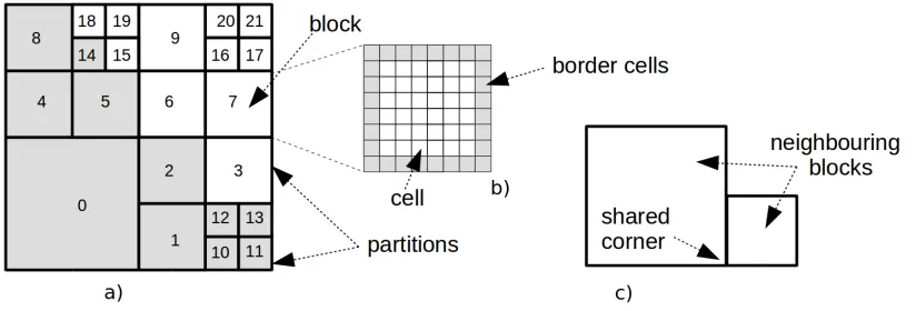
The domain subdivision is done by means of aBlock Uniform Quad-Treegrid (BUQ) [6]. Our definition of BUQ relies on the notion ofquadtree subdivisiongiven in [4] with some adaptation to our specific problem. A BUQsubdivisionis aquadtree subdivision, Figure1-a), in which eachleafof the quadtree is a matrixM×M- Figure1-b) - whereM is constant for all leaves (in our models we useM ∈ {8,16}). We call blocksuch matrix andcells the entries of the matrix. Each cell represents a square surface whose dimension is2i∆for0 ≤i < kwhere∆ ∈
Randk ∈N+are fixed. The integeriidentifies theresolutionof a block. Blocks sharing at least onecornerare calledneighboursoradjacentblocks, Figure1-c). Furthermore, we impose an important constraint on our spatial subdivision: each pair of adjacent blocks can differ for at most one resolution level.
The memory representation of a BUQ grid can be seen as a bidimensional array tiled up with blocks having an unique identifier calledindex. Let us note that this representation does not preserve neighbour-ing relations between blocks [6](i.e., two adjacent blocks in the BUQ can be far away from each other in memory). Thus for keeping track of adjacency relations between blocks a directed graphG(S, E)is defined, whereSis a set ofindexesandEis the set of pairs(i, j), wherei, j∈Sandi, jareneighbours. The simulation is performed on Nvidiagraphic processing units(GPUs) which are able to spawn thousands of conurrent threads. In the NVIDIATM Compute Unified Device Architecture (CUDA)
Figure 1: a) Quad Tree Subdivision of a domain in22blocks. The set of blocks is split into two partitions respectively highlighted whit white and grey areas. b) Each block is a matrix ofM ×M cells, where M is the same for all blocks. c) Neighbours blocks share a corner.
There is a one-to-one mapping between the CUDA environment and our spatial models, namely each spatial block is mapped into a CUDA block and each computational cell is mapped into a CUDA thread. Although a GPU offers the possibility to perform a high number of calculations in parallel, the simulation time can still be unsatisfactory for input grids having order of106-107cells. Furthermore, the memory of a single GPU (up to 16GB) is rather limited for our application and so is the dimension of the input models. To overcome these limitations, the Section4presents an extension of the PARFLOOD simulator [6] which takes advantage of the spatial decomposition to perform Multi GPU simulations over a network.
Example 3.1. In Figure1the set of block indexes isS ={0,1, . . . ,21}. The neighbors of the block
1are0,2,3,10,12. Each block has8×8 = 64 cells. The GPU simulation spawns22×64CUDA threads, each one computing the content of a cell based on the content of neighboring cells.
4
Multi GPU Implementation
In Section3a single GPU implementation of theshallow water equationssolver has been briefly dis-cussed. The aim of this section is to generalize the single GPU implementation to a scalable multi GPU version. While the former version stores the domain and the related data structures on a single GPU, the latter version decompose the global domain into different pieces, calledpartitions. Each partition is then assigned to a different GPU. The preprocessing stage presented in Section 4.1describes the data structures which allow different partitions to exchange border information. In Section4.2a multi GPU algorithm is discussed. Finally, the Section4.3evaluates the performances of the algorithm by presenting both strong and weak scalability tests.
4.1
Preprocessing Stage
Before describing in detail the preprocessing stage, let us introduce some notation that will help to make the description more clear. The symbolS denotes the set of blocks indexes in a domain and will be referred to as the global set of blocks. The multi GPU implementation is done by partitioning the set Sinto a sequence of non-empty disjoint setsS1, . . . , Snwherenis the number of processes over which
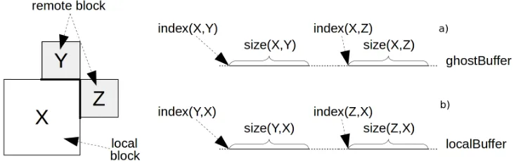
Figure 2: a) Mapping of remote blocks Y and Z into the ghostBuffer inside an area reserved for X readings. b) Mapping of local block X into the localBuffer which is sent to the partitions containing Y and Z.
note thatnis an input to the multi GPU simulation and does not change during the computation. Each partitionStis simulated on a different nodeptequipped with a GPU. Recall that a global domain can be
represented by means of an adjacency graphG(S, E), whereS denotes the global set of blocks andE denotes the neighboring relations between blocks. The notationneigh(b)indicates the set of neighbors of a blockb∈S. We further assume that the global domain isstatically partitionedintonsets (i.e., the content of each partition does not change during the simulation).
During the partitioning stage, a blocks distribution tableT is computed for keeping track of the distribution of blocks among different partitions. Formally, for each blockb ∈S,T(b) =tif and only ifb ∈St. In our implementationtis an integer, calledrank, which uniquely identifies the processpt.
During the preprocessing stage further information is to be computed to allow neighboring domains to exchange border information. With this purpose each processptcreates three different disjoint sets
which we callinternalBlocks,borderBlocks,ghostBlocks. The first is the set of blocksb∈Stsuch that
all neighbors ofb belong toSt( i.e., neigh(b) ⊂ St). The second is the set of blocks b ∈ Stsuch
thatbhas at least one remote neighbor, (i.e.,∃r∈neigh(b)s.t. r /∈St). The third is the set of blocks
r∈S\Sts.t. rhas at least one neighbor inSt(i.e.,∃b∈neigh(r)s.t.b∈St).
This implementation does not need any assumption on how blocks are distributed among different partitions, however we prefer to minimize exchanged boundaries by using partitions with a single self-avoiding closed fronteer (Figure1-a).
Example 4.1. In Figure1the global set of blocks isS = {0, . . . ,21}. The domain is split into two partitions,S1={0,1,2,4,5,8,10,. . . ,14}simulated on nodep1, andS2=S\S1, simulated on node p2. The set of blocks associated with the partitionS1areinternalBlocks={0,4,10,11},ghostBlocks=
{3,6,7,9,15,18,19}andborderBlocks={1,2,5,8,12,13,14}. For allb ∈S1 T(b) = 1and for all b∈S2T(b) = 2.
During the preprocessing stage, each processptdefines two distinct memory buffers, theghostBuffer
for storing information received from remote partitions and thelocalBuffer for writing local border information which needs to be sent to remote partitions. (Figure2).
We detail how to precompute some additional information, in order to let each each block efficiently locate the correct offset insideghostBuffer(resp. localBuffer) where to read (resp. to write) the data received from (resp. to send to) some remote block. For this purpose, we introduce theremote adjacency mapwhich is computed for each partitionSt(see Example4.2). In particular, given a partitionSt, for
(y, coord, index(x,y), size(x,y)). The number of tuples stored inLt(x)is equal to the number of remote
neighbors ofx. The first elementyindicates a remote neighbor block located at the coordinatecoord from the point of view ofx. Ifxis local toStthenindex(x,y)indicates the offset insidelocalBuffer where the information aboutxhas to be written and sent to the blocky. Otherwise, ifxis not local to St,index(x,y)indicates the offset inside theghostBufferwhereyhas to to read the information aboutx received from a remote partition. The last element,size(x,y), indicates either the number of grid cells to write into thelocalBuffer(ifxis local), or the number of grid cells to read from theghostBuffer(ifxis remote). Let us note thatLt(x)can be also the empty list, which means that the blockxdoes not have
any remote neighbors. Once a mapLthas been computed for each partitionSt, the information about
how to read and writeghostBufferandlocalBufferis known. Notice that is also implicitly known how much space must be allocated for each one of these buffers. In particular, the length of theghostBuffer
is the sum of thesizeelements of each tuplet∈L(x), for allx∈ghostBorder. Similarly, the length of thelocalBufferis the sum of thesizeelements of each tuplet∈L(x), for allx∈localBorder.
Example 4.2. In Figure2a local blockxand two remote blocksy, zare shown. The mapL(x)contains the tuples(y, N, index(x, y), size(x, y))and(z, E, index(x, y), size(x, y))which tellxhow to read yandzfrom theghostBuffer. The mapL(y)contains the tuple(x,S, index(y, x),size(y, x))andL(z)
contains the tuple(x, W,index(z, x), size(z, x))which tellsxhow to write information foryandzin thelocalBuffer. Notice thatyandzmay belong to two different partitions.
Each process builds his own remote adiacency map with a local viewpoint. When exchanging buffers, a certain processptneeds to know how other processes will pack and send their local
infor-mation. To address this, we let adjacent partitions exchange their respective maps before the the simula-tions starts. In this way a nodeptcan send directly hislocalBufferto each neighbor, which in turn uses
the map belonging toptto read it, and their local map to save the data into theirghostBuffer. If on one
hand this method simplifies the implementation of the communication procedures, on the other hand it increases the network overhead of a factor proportional to the number of neighbors of the sending node. However we will show that such overheads are small and completely maskable by the computation of the GPU kernels.
4.2
Simulation Stage
The Listing1shows the pseudocode of the multi GPU implementation. Only the simulation halfstep is described as our main goal is to discuss the communication between different processes. For a complete version of the PARFLOOD implementation on a single GPU, please refer to [6].
Listing1: Simulation Halfstep of the Multi GPU Implementation 1 / / D e l t a T c a l c u l a t i o n
2 d t = g p u d e l t a T ( ) ;
3 / / Compute t h e minimum d e l t a T among a l l p a r t i t i o n s ( b l o c k i n g c a l l ) . 4 d t m i n = d e l t a T R e d u c t i o n ( d t ) ;
5 / / BDO p r o c e d u r e
6 d e f i n e w e t t a b l e b l o c k s ( ) ;
7 / / MUSCL R e c o n s t r u c t i o n f o r i n t e r n a l b l o c k s 8 g p u m u s c l r e c o n s t r u c t i o n ( i n t e r n a l B l o c k s ) ; 9 / / S e n d i n g and r e c e i v i n g t h e c o n s e r v e d v a r i a b l e s 10 c o m m u n i c a t i o n ( l o c a l B u f f e r , g h o s t B u f f e r ) ; 11 / / MUSCL R e c o n s t r u c t i o n f o r b o r d e r b l o c k s 12 g p u m u s c l r e c o n s t r u c t i o n ( b o r d e r B l o c k s ) ;
13 / / U p d a t e C o n s e r v e d V a r i a b l e s f o r i n t e r n a l b l o c k s , f l u x and s o u r c e t e r m s 14 g p u f l u x e s c a l c u l a t i o n ( i n t e r n a l B l o c k s ) ;
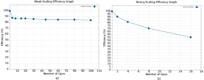
Figure 3: a) Resoluts of weak scalability tests up to100GPUs performed over a uniform resolution BUQ grid. b) Resoults of strong scalability tests performed over a circular dam break discretized using a multi resolution BUQ grid.
17 / / U p d a t e C o n s e r v e d V a r i a b l e s f o r b o r d e r b l o c k s , f l u x and s o u r c e t e r m s 18 g p u f l u x e s c a l c u l a t i o n ( b o r d e r B l o c k s ) ;
At the beginning of the temporal loop, the timestep∆t has to be calculated by each partition (line 2), and then an MPI reduction has to be performed in order to obtain the global minimum value (line 4). Since all the processes have to wait the response from the master process, this call represents the only one which can not be masked. The call plays a critical role in the execution time, especially if the computational load between different GPUs is unbalanced. The other communication calls (line 10, 16) are performed in a point-to-point nonblocking fashion, without the need to synchronize thesendcalls with thereceivecalls among neighbors. Instead, one process can perform all thesendcommunications and then wait for all the remote data to arrive. In line10the local borderreconstructed variablesstored in thelocalBuffer are sent to the neighbor processes. Similarly remote reconstructed variables are received from neighbor processes into thelocalBuffer. The same thing happens for the communication performed in line 16, with the only difference that the buffers contain theconserved variables. Thanks to the asynchronous nature of GPU kernels, both the MUSCL reconstruction (line 8) and the Fluxes integration kernels (line 14) can execute concurrently with the communication calls right after them. This can be done because such kernels execute oninternalBlocks, thus they don’t need the border data. Once the MPI communication has been completed, CUDA kernels which operate onghostlBlockscan be executed. In Section4.3we discuss the performance of this algorithm.
4.3
Numerical Tests
To assess the performance of our code we preformed bothstrongandweakscalability tests on the Piz Daint supercomputer located at the Swiss National Super Computing Centre. Piz Daint is an hybrid Cray XC40/XC50 system equipped with NVIDIA P100. Our GPU code has been tested on CUDA 8 and cray-mpich 7.6 as MPI implementation.
The weak scaling test shown in Figure3-a has been performed by defining a fixed partition size of
small degradation which keeps the efficiency around85%up to100GPUs. By profiling the code with
nvprof we show that asynchronous communication steps (i.e., lines10and16of the Listing1) do not affect the simulation time at all. The drop of efficiency is entirely caused by the reduction performed at line4(plus some minor overheads caused by data exchange between CPU and GPU).
The strong scalability test has been performed over a circular dam break model, containing a total of24700blocks (i.e≈6.3·106cells). For this test a BUQ grid (Section3) is used and the partitioning is performed along one dimension. We enforce that each partition contains the same number of blocks. Figure3-b shows that the efficiency dropdown varies from10to15%by doubling the number of GPUs. By profiling our code withnvprofwe noticed that the main factor which causes the loss of efficiency is the 1D partitioning. In fact, by doubling the number of GPUs involved in the simulation, the number of blocks is halved for each partition, however the the size of the borders remains almost the same (i.e., a small variation can happen due to the multiresolution grid). Thus the running time for the border kernels (lines12and18in the Listing1) remains constant. Another factor which causes a loss of efficiency is related to the computational load of the kernels which execute on internal blocks (lines8and14). In particular we observed that those kernels stick to an efficiency of100%as long as there are at least
3000blocks for each partition. This explains the efficiency dropdown increase for a number of GPUs higher than8. The network overhead is caused only by the synchronization time, especially for2and
4GPUs and then it becomes negligible. Instead, the asynchronous communication (lines10and16) is completely masked by kernel execution, thus it does not affect the execution time, supporting our choice to send all the border data to each partition.
References
[1] M. Asunci´on, M.J. Castro, E. Fern´andez-Nieto, J.M. Mantas, S.O. Acosta, J.M. Gonz´alez-Vida (2013). Effi-cient gpu implementation of a two waves tvd-waf method for the two-dimensional one layer shallow water system on structured meshes, Comput. Fluids 80, 441-452
[2] A.R. Brodtkorb, M.L. Sætra, M. Altinakar (2012). Efficient shallow water simulations on GPUs: Implemen-tation, visualization, verification and validation Comput. Fluids 55, 1-12
[3] NVIDIA CUDA, 2018, CUDA C Programming Guide. docs.nvidia.com/cuda/cuda-c-programming-guide/index.html
[4] M. de Berg, O. Cheong, M. van Kreveld, M. Overmars, 2008, Computational Geometry. Algorithms and Applications. Third Edition. Springer. 313–314.
[5] E.F. Toro (1999). Shock Capturing Methods for Free Surface Shallow Water Flows. Wiley, New York. [6] R. Vacondio, A. Dal Pal`u, A. Ferrari, P. Mignosa, F. Aureli, S. Dazzi (2017). A non-uniform efficient grid
type for GPU-parrallel Shallow Water Equations models. Adv. Water. Resour. 88, 119-137
[7] R. Vacondio, A. Dal Pal`u, P. Mignosa, (2014). GPU-Enhanced Finite Volume Shallow Water solver for fast flood simulations. Environ. Model. Softw. 57, 60-75.