Multiple Solutions for the Riemann Problem in the Porous Shallow Water Equations

Multiple solutions for the Riemann problem in

the Porous Shallow Water Equations

Luca Cozzolino

_{, Raffaele Castaldo}

_{, Luigi Cimorelli}

_{, Renata Della}

Morte

_{, Veronica Pepe}

_{, Giada Varra}

_{, Carmine Covelli}

_{and Domenico}

Pianese

1 _{Dipartimento di Ingegneria – Università degli Studi di Napoli Parthenope, Centro Direzionale di}

Napoli Isola C4, Napoli 80143, Italy

2 _{LA SIA Srl, via L. Schiavonetti 286, Roma 00173, Italy.}

3 _{Dipartimento di Ingegneria Civile, Edile e Ambientale – Università degli Studi di Napoli}

Federico II, via Claudio 25, Napoli 80125, Italy.

[email protected], [email protected], [email protected]

Abstract

The Porous Shallow water Equations are widely used in the context of urban flooding simulation. In these equations, the solid obstacles are implicitly taken into account by averaging the classic Shallow water Equations on a control volume containing the fluid phase and the obstacles. Numerical models for the approximate solution of these equations are usually based on the approximate calculation of the Riemann fluxes at the interface between cells. In the present paper, it is presented the exact solution of the one-dimensional Riemann problem over the dry bed, and it is shown that the solution always exists, but there are initial conditions for which it is not unique. The non-uniqueness of the Riemann problem solution opens interesting questions about which is the physically congruent wave configuration in the case of solution multiplicity.

1

Introduction

The Shallow water Equations are widely used to study urban flooding events. These hyperbolic partial differential equations are non-linear, and admit the existence of discontinuities (moving bores, standing hydraulic jumps, wetting-drying boundaries) that develop in finite time, also if the initial conditions are smooth, i.e. continuous with higher-order derivatives [1, 2]. The Riemann problem is a special initial value problem where the initial conditions are discontinuous, and it is used to model the cited flow field discontinuities [1, 2].

Volume 3, 2018, Pages 476–484

Modern numerical models for the simulation of flooding phenomena are often based on the approximate or exact solution of the classic Riemann problem for the Shallow water Equations, which always exists and it is unique [1]. The solution of the Riemann problem on dry bed [3] has started the modern approaches in the evaluation of flooded areas extent. This solution, which inherits the uniqueness property from the general Riemann problem, exhibits a very simple structure, because it consists of a single rarefaction wave that connects the left state with the right dry bed [1, 3].

In the urban environment, the numerical calculations are very time consuming, because the modelling of building geometric details requires fine computational grids [4]. In order to reduce the computational burden, an alternative approach based on the Porous Shallow water Equations [5, 6, 7] has been introduced. In this approach, which corresponds to the averaging methods used for multiphase flows [8], the solid obstacles are implicitly taken into account by averaging the classic Shallow water Equations on a Representative Elementary Volume containing the fluid phase and the obstacles [5, 7]. In the single-porosity models, which are the object of the present paper, the fraction of the unit-surface area that is not occupied by obstacles is called porosity [5, 6, 7]. It is possible to demonstrate that the Porous Shallow water Equations are non-linear and hyperbolic [6, 9], and then may exhibit discontinuities. Moreover, a rotational invariance property is satisfied [6].

In realistic applications, the porosity can be discontinuous, because the fraction of the urban areas occupied by buildings can be strongly variable in space, and this leads to the open question about the influence of geometric discontinuities on the solution of the Riemann problem for the Porous Shallow water Equations. Despite the existence of some example solution (see, for example, [6, 9, 10]), there is not a systematic study of the general Riemann problem for the Porous Shallow water Equations.

It is possible to demonstrate [11] that the solution of the dam-break problem, i.e. the particular case of Riemann problem with initial zero velocity, depends on the definition of the geometric-discontinuity inner-structure. In particular, most of the existing geometric geometric-discontinuity definitions, such as those contained in [6] and [10], may lead to unphysical solutions (increase of the flow energy through the discontinuity). Other definitions, such as those by [12] and [13], are either internally inconsistent or imply the incompleteness of the problem solution. Interestingly, the solution of the dam-break problem always exists and it is unique if an appropriate parameterization of the stationary weak solutions of the Porous Shallow water Equations is used to supply the inner structure of the geometric discontinuity, as made in [11].

In the present paper, the exact solution of the one-dimensional Riemann problem for the Porous Shallow water Equations is presented, assuming that the right state is initially dry and that the jump definition is the same of [11]. This special Riemann problem on dry bed seems a good candidate in order to explore interesting problems encountered when the flooding of urban areas with strong porosity gradients and initial dry bed is modelled.

2

The position of the Riemann problem for the Porous

Shallow water Equations

The rotational invariance of the two-dimensional Porous Shallow water Equations allows considering the one-dimensional framework

, (1)

where the following discontinuous initial conditions are considered:

( ) ( )

t x x

f

f ¶ f

¶ _{+ +} ¶ ₌

¶ ¶ ¶

f u u

. (2)

In Eqs. (1)-(2), the symbols are defined as follows: x is the space variable, t is the time variable, h(x, t) is the water depth, u(x, t) is the depth-averaged velocity, is the vector of the flow

conserved variables, is the vector of the fluxes, is

a vector that takes into account the porosity gradients effect, and are the initial left and right flow states, while φ(x) is the porosity. The aspect ratio AR is defined as the ratio between the right and the left porosity, that is .

In order to consider the Riemann problem on dry bed, in the following it will be assumed that the state coincides with the dry bed state . This implies that the flow through the geometric discontinuity is always directed from left to right.

2.1

The porosity discontinuity

The porosity discontinuity induces a standing flow discontinuity at x = 0 for t > 0. This standing discontinuity, where the non-conservative product is active, is not autonomous [14], and the missing physical information must be supplemented. Congruently with [11], it is assumed here that the states and , immediately to the left (x = 0-_{) and to the right}

(x = 0+_{) of the geometric discontinuity in x = 0, are connected by a stationary solution of Eq. (1). This}

means that the flow energy is conserved through the geometric discontinuity, unless a hydraulic jump is present. In addition, it is assumed that φ varies monotonically through the porosity jump. This means that critical state conditions can be attained only at the left (AR ³ 1) or at the right (AR < 1) of the geometric discontinuity. In the following and are the Froude numbers corresponding to the states and , respectively.

2.2

Ritter solution (AR = 1)

When the porosity discontinuity is absent (AR = 1), the solution of the Riemann problem on the dry bed consists of a unique rarefaction wave contained in the first characteristic field that connects the left state to the dry bed state , while . Along the rarefaction, the velocity and the fluid depth are constrained by [1, 2]

(3)

and

, (4)

where . In particular, the left and the right edges of the rarefaction wave have speed and , respectively, with . The velocity u increases (

( )

( )

, 0 , 0

L L R R x x x x x x f f f < < ì ì =_í =_í > > î î u u u

(

)

h hu

=

u

( )

(

)

f u _{h u}

( )

(

)

(

)

u

(

)

R = hR h uR R

u

R L

AR=

f f

R

u 0=

(

)

2

h ¶ ¶

f

(

)

1 1 1 1

T

h h u

=

u 2

(

)

T h h u =

u

1 1 1

F =u gh F₂=u₂ gh₂

1

u u₂

L

u u_R=0 u₁=u₂

2 _L 2 _L

u+ gh u= + gh

( )

l

( )

1 u gh

l u =

) along the rarefaction from the left edge ( ) to the right edge ( ), while the flow depth decreases ( ) from the left edge ( ) to the right edge (h = 0). If is the Froude number corresponding to the left state , it is easy to see that the Froude number increases continuously from the value at the left edge, and tends to infinity at the right edge.

The Froude number rules the following three cases:

Case Ra. When , the rarefaction wave develops entirely to the left of x = 0 because is negative, and u < 0 everywhere. In this case, u1 = 0.

Case Rb. When , the wave develops through x = 0 because and . The eq. (4) implies that critical flow conditions are obtained in x = 0, with flow velocity directed

from left to right. In this case .

Case Rc. When , the rarefaction wave develops entirely to the right of x = 0 because is positive. This implies that for x £ 0. In addition, the velocity u is positive everywhere, and the flow is supercritical.

2.3

Energy limit

When u1 > 0, a necessary condition for the flow to be smooth through the geometric discontinuity

is that the energy of the incoming flow u1 is not less than the minimum energy (critical state) required

at the outlet. This implies that the constraint

, (5)

is satisfied. From the study of eq. (5) it follows that:

(a) AR ³ 1 is required when F1 = 1, and this means that the critical flow cannot freely pass

through a porosity decrement.

(b) The eq. (5) is satisfied by any value of F1 for AR ³ 1. In other words, any flow is able to pass

through a porosity increment.

(c) When AR < 1, the eq. (5) is satisfied by the values , where and are two limits depending on AR, with and

. The values or at the inlet of the porosity discontinuity satisfy the eq. (5) with the equality sign, and imply at the outlet of the porosity decrement.

2.4

Hydraulic jump limit for supercritical flows

When AR < 1, it is interesting to consider the case where critical flow conditions are obtained at the exit of the discontinuity ( ), while a subcritical stationary flow profile develops through the geometric discontinuity and . The supercritical flow connected by a standing hydraulic jump to the subcritical flow at the inlet of the geometric discontinuity satisfies the limit condition

0 u x

¶ ¶ > u u= _L u u= _L+2 gh_L

0 h x

¶ ¶ < h h= _L

L L L

F =u gh uL

F u= gh F F= _L

L

F 2

L

F £ - sR

2 F_L 1

- < £

s

s

u= gh

(

)

(

)

(

)

1 2 9 2 27

T

L L L L

h F gh F

= + +

u

1

L

F > sL

1= L

u u

2 2 3 2 3

1 1

2₊F _³3AR- F

( )

( )

1 0, sub sup ,

FÎù_û F AR ù_{û ë}ÈéF AR ¥é_ë

( )

sub

F AR F_sup

( )

( )

( )

sup 1

F AR > F₁=F_sub

( )

( )

2 1 F =

2 1 F =

( )

. (6)

The supercritical flow with Froude number less than is not able to sustain a hydraulic jump at the inlet of the sudden porosity decrement, and a shock moving upstream may be obtained.

2.5

Hydraulic hysteresis region

If the equality sign and FL = F1 are taken in eq. (5), the limit condition

, (7)

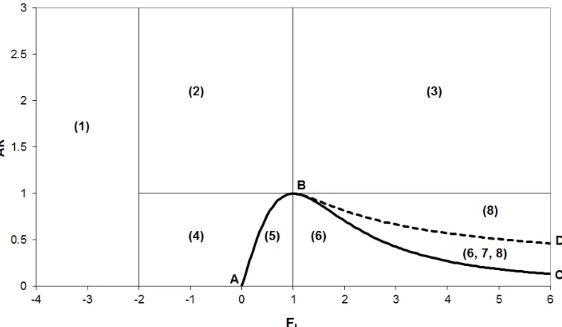
is obtained [15]. The eq. (7) is represented in Figure 1 (continuous black line), and the corresponding graph consists of a subcritical reach AB and a supercritical reach BC. Based on eq. (5), the points of the plane (FL, AR) above the energy limit curve of eq. (7) refer to flows uL that are able to pass through the geometric discontinuity remaining smooth.

If is taken, the eq. (6) can be solved with respect to . Recalling that satisfies eq. (5) with the equality sign, the following limit condition [16, 17] is obtained

. (8)

The corresponding curve, which is plotted in Figure 1 (curve BD with dashed black line), lies above the energy limit curve ABC. Based on eq. (6), the points of the plane (FL, AR) below the standing hydraulic jump limit BD are referred to supercritical flows that do not pass through the geometric discontinuity, because they are turned into subcritical states by a backward moving shock [16, 17].

The region of the plane between the curves BC and BD admits both an upstream supercritical flow passing through the discontinuity (above BC) and a supercritical upstream flow that is turned in subcritical (below BD). This phenomenon is called hydraulic hysteresis [16, 17]. Interestingly, in the hysteresis region, a third flow condition is possible, namely a standing hydraulic jump through the geometric discontinuity, where the upstream supercritical flow is turned in subcritical [17].

3

Solution configurations for the Riemann problem with right

dry state

Depending on the left Froude number FL and on the aspect ratio AR, eight different solution configurations for the Riemann problem on dry bed are possible. These solution configurations, whose fields of existence are plotted in Figure 1, are listed as follows.

( )

( )

( )

2

2

1 8 3

jump sub

sub

F AR F AR

F AR æ ö ç ÷ = _{ç ÷} + -è ø

( )

3 2 ₂

3 1 2 2 L L F AR F -æ ö æ ö = ç ÷ ç + ÷ è ø è ø

( )

F =F AR F_sub

( )

( )

F =F AR

(

)

(

)

3 2 3 2

3 2 2

2

1 8 3

3 ₁

2 2 _{16 1 8 1}

3.1

Solution configuration not depending on AR

SC (1). In this solution configuration, the condition is satisfied, and the solution configuration coincides with the Case Ra of subsection 2.2. A rarefaction wave develops entirely to the left of the geometric discontinuity, and the velocity u is non-positive everywhere. In other words, there is not interaction between the flow and the geometric discontinuity.

Figure 1: Field of existence of the solution configurations.

3.2

Solution configurations with AR

³

1 (sudden porosity increment)

In this group of solution configurations, the flow corresponding to the Ritter solution (Case Rb and Case Rc of subsection 2.2) immediately to the left of x = 0 encounters a sudden porosity increment. For this reason, the geometric discontinuity is not an obstacle to the flow.

SC (2). In this solution configuration, (Case Rb). A rarefaction connects the state uL to the critical state u1, and the energy of the flow is sufficient to pass through the geometric discontinuity

because F1 = 1 satisfies the eq. (5) with AR ³ 1. The supercritical state u2 is connected to u1 by means

of the conditions of energy and discharge conservation. Finally, the dry bed state uR is connected to u2

by means of a rarefaction.

SC (3). In this solution configuration, (Case Rc). The state u1 coincides with the

supercritical state uL, and the energy of the flow is sufficient to pass through the geometric discontinuity because F1 > 1 satisfies the eq. (5) with AR ³ 1. The supercritical state u2 is connected

to u1 by means of the conditions of energy and discharge conservation, while a rarefaction connects

the state u2 to the dry bed.

2

L

F £

-2 F_L 1 - < £

1

3.3

Solution configurations with AR < 1 (sudden porosity decrement)

SC (4). In this solution configuration, (Case Rb). A rarefaction connects the state uL to the subcritical state u1, which is characterized by . The state u2 is critical,

and it is connected to u1 by means of the conditions of energy and discharge conservation. Finally, the

state state u2 is connected to the dry bed by means of a rarefaction.

SC (5). In this solution configuration, (Case Rb). A shock moving upstream connects the subcritical (or critical) state uL to the subcritical state u1, which is characterized by

. The state u2 is critical, and it is connected to u1 by means of the conditions of energy

and discharge conservation. Finally, the state state u2 is connected to the dry bed by means of a

rarefaction.

SC (6). In this solution configuration, (Case Rc). A shock moving upstream (if ) or standing in x = 0- _{(if ) connects the supercritical state uL to the}

subcritical state u1, which is characterized by . The state u2 is critical, and it is

connected to u1 by means of the conditions of energy and discharge conservation. Finally, the critical

state u2 is connected to the dry bed by means of a rarefaction.

SC (7). In this solution configuration, (Case Rc). The state u1

coincides with the supercritical state uL, while the critical state u2 is connected to u1 by means of the

conditions of discharge conservation only, and a hydraulic jump is located through the geometric discontinuity. Finally, the critical state u2 is connected to the dry bed by means of a rarefaction.

SC (8). In this solution configuration, (Case Rc), and the flow is free to pass through the porosity decrement. The state u1 coincides with the supercritical state uL. The state u2 is

connected to the state u1 by means of the conditions of energy and discharge conservation. A

rarefaction wave, which connects the supercritical state u2 to the dry bed, develops entirely on the

right of the geometric discontinuity.

4

Discussion

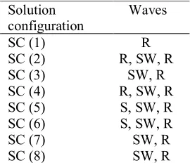
The solution of the Riemann problem on the dry bed for the classic Shallow water Equations is unique, and consists of a rarefaction wave connecting the left state to the right dry bed. Conversely, the Riemann problem on the dry bed for the Porous Shallow water Equations may exhibit numerous solution configurations, which differ for the type of waves, as well their number and position. The Table 1 resumes these solution configurations, described in the Section 3, using the following symbols: R = rarefaction wave, SW = standing wave (geometric discontinuity), S = shock.

The direct calculations show that the solution of the Riemann problem always exists for given flow initial conditions and geometric discontinuity characteristics. Nonetheless, there are cases where this solution is not unique (bifurcation phenomenon), and the inspection of Figure 1 confirms that there is a field of the plane (FL, AR) where three distinct solution configurations (SC (6), SC (7), and SC (8)) are possible for given initial conditions and geometric discontinuity characteristics. From a physical point of view, this field coincides with the case where the supercritical incoming flow has energy greater than that strictly required to pass through the porosity reduction, and this energy can be dissipated through a standing hydraulic jump or a moving shock. These solutions are the unsteady flow counterparts of the multiple steady states in converging channels [16, 17].

( )

2 F_L F_sub AR - < £

( )

1 sub F =F AR

( )

sub L

F AR <F £

( )

1 sub F =F AR

( )

( )

1<F_L<F_jump AR F_L=F_jump

( )

( )

F =F AR

( )

( )

sup L jump

F AR £F £F AR

( )

sup L

The non-uniqueness of the Riemann problem solution is expected in the case that geometric discontinuities are present, and it is well documented in the context of the Shallow water Equations with a bed step [18, 19].

5

Conclusions

The solution of the Riemann problem over the dry bed for the Porous Shallow water Equations always exists, and the main parameters on which it depends are the initial left Froude number FL and the aspect ratio AR, i.e. the ratio between the right and the left porosity. In addition, it is demonstrated that, contrarily to the case of the classic Shallow water Equations (Ritter solution), numerous different wave configurations are possible for t > 0, despite of the very simple initial conditions. These flow configurations differ for the number and the type of waves exhibited by the solution.

Interestingly, there are values of FL and AR for which the problem solution is not unique, and multiple flow configurations are possible. This phenomenon, which appears for supercritical left states, has never been documented in the context of the Porous Shallow water Equations. The non-uniqueness of the solutions opens interesting questions about which is the physically congruent wave configuration in the case of solution multiplicity, and about the foundations of the Porous Shallow water Equations themselves.

6

Acknowledgement

This research was partially funded by the University of Naples Parthenope through the funding programs “Sostegno alla Ricerca individuale 2015-2017” and "Ricerca competitiva triennio 2016-2018".

References

[1] E.F. Toro, Shock-capturing methods for free-surface shallow flows. Wiley, Chichester, 2001. [2] R.J. LeVeque, Finite Volume Methods for Hyperbolic Problems. Cambridge University Press, Cambridge, 2012.

[3] A. Ritter, Die Fortpflanzung der Wasserwellen, Vereine Deutscher Ingenieure Zeitswchrift 36 (1892) 947-954 (in German).

Solution

configuration Waves

SC (1) R

SC (2) R, SW, R

SC (3) SW, R

SC (4) R, SW, R SC (5) S, SW, R SC (6) S, SW, R

SC (7) SW, R

SC (8) SW, R

[4] B. Kim, B.F. Sanders, J.S. Famiglietti, V. Guinot, Urban flood odelling with porous shallow-water equations: a case study of model errors in the presence of anisotopic porosity, Journal of Hydrology 523 (2015) 680-692.

[5] A. Defina, Two-dimensional shallow flow equations for partially dry areas, Water Resources Research 36 (2000) 3251-3264.

[6] V. Guinot, S. Soares-Frazão, Flux and source term discretization in two-dimensional shallow water models with porosity on unstructured grids, International Journal for Numerical Methods in Fluids 50 (2006) 309-345.

[7] M. Velickovic, Macroscopic modeling of urban flood with a porosity model. Doctoral thesis, Université Catholique de Louvain, Louvaine-la-Neuve, 2012.

[8] M. Hassanizadeh, W.G. Gray, General conservation equations for multi-phase systems: 1. Averaging procedure, Advances in Water Resources 2 (1979) 131-144.

[9] A. Ferrari, R. Vacondio, S. Dazzi, P. Mignosa, A 1D - 2D Shallow Water Equations solver for discontinuous porosity field based on a Generalized Riemann Problem, Advances in Water Resources 107 (2017) 233-249.

[10] S. Ion, D. Marinescu, A.V. Ion, S.G. Cruceanu, A shallow water model for hydrodynamic processes on vegetated hillslope. Water flow modulus. arXiv:1512.00706, 2015.

[11] L.Cozzolino, V. Pepe, L. Cimorelli, A. D’Aniello, R. Della Morte, D. Pianese, The solution of the dam-break problem in the Porous Shallow water Equatinos, Advances in Water Resources 114 (2018) 83-101.

[12] M.J. Castro, A. Pardo Milanés, C. Parés, Well-balanced numerical schemes based on a generalized hydrostatic reconstruction technique, Mathematical Models and Methods in Aplied Sciences 17 (2007) 2055-2113.

[13] V.V. Ostapenko, Dam-break flows at a jump in the width of a rectangular channel, Journal of Applied Mechanics and Technical Physics 53 (2012) 679-689.

[14] G. Dal Maso, P.G. LeFloch, F. Murat, Definition and weak stability of nonconservative products, Journal de Mathématiques Pures et Appliqués 74 (1995) 483-548.

[15] D.L. Yarnell, Bridge piers as channel obstructions, Technical Bulletin 444, US Department of Agriculture, Washington, 1934.

[16] A. Defina, F.M. Susin, Multiple states in open channel flow, in: Vorticity and Turbulence Effects in Fluid Structures Interactions, Advances in Fluid Mechanics, M. Brocchini, F. Trivellato (Eds.), Wessex Institute of Tehcnology Press, Southampton 2006, pp. 105-130.

[17] B. Akers, O. Bokhove, Hydraulic flow through a channel contraction: multiple steady states. Physics of Fluids 20 (2008) 056601.

[18] P.G. LeFloch, M.D. Thanh, A Godunov-type method for the shallow water equations with discontinuous topography in the resonant regime. Journal of Computational Physics 230 (2011) 7631-7660.