Volume 9, 2018, Pages 37–48
LPAR-22 Workshop and Short Paper Proceedings
Extending a Verified Simplex Algorithm
Ren´
e Thiemann
University of Innsbruck
Abstract
As an ingredient for a verified DPLL(T) solver, it is crucial to have a theory solver that has an incremental interface and provides unsatisfiable cores. To this end, we extend the Isabelle/HOL formalization of the simplex algorithm by Spasi´c and Mari´c. We further discuss the impact of their design decisions on the development of our extension.
1
Introduction
CeTA[BJTY17] is a verified certifier for checking untrusted safety and termination proofs from external tools such asAProVE [GAB+17] andT2 [BCI+16]. To this end, CeTAalso comprises a verified SAT-modulo-theories (SMT) solver, since these untrusted proofs contain claims of validity of several formulas.
The ultimate aim of this work is the optimization of the existing verified SMT solver, because the current solver is quite basic. It takes as input an arbitrary formula in the theory of linear integer arithmetic (LIA), translates it into disjunctive normal form (DNF), and then tries to prove unsatisfiability of each conjunction of literals in the theory of linear rational arithmetic (LRA) with the verified simplex implementation of Spasi´c and Mari´c [SM12]. This basic solver has at least two limitations. It only works on small formulas, since the conversion to DNF easily leads to an exponential blowup; and the procedure is incomplete because of the switch from LIA to LRA.
The second limitation was not a limiting factor up to now, i.e., all formulas in the certificates ofAProVEandT2have even been valid in LRA. On the other hand, there exist proofs ofAProVE
andT2 where certificate checking with the verified SMT solver requires more than a minute. Clearly, instead of the expensive DNF conversion, the better approach is to verify an SMT solver which is based on DPLL(T) or similar algorithms [GHN+04,BGS18].
Although there has been recent success in verifying a DPLL based SAT solver [BFLW18], for DPLL(T) a core component is missing, namely a powerful theory solver. Therefore, in this paper we will extend the formalization of the simplex algorithm so that in the future it can be combined with a DPLL algorithm to obtain a fully verified DPLL(T) based SMT solver. We describe two main features of our work.1
• Instead of just delivering an unsatisfiability flag as result, we return unsatisfiable cores.
1The third feature is an optimization of Dutertre and de Moura that has not been formalized by Spasi´c and
• We provide an incremental interface to the simplex method. It permits incremental as-sertion of constraints, backtracking, etc.
Our formalization is completely based on the incremental simplex algorithm described by Dutertre and de Moura [DdM06]. This paper was also the basis of the existing implementation by Spasi´c and Mari´c, of which the correctness has been formalized in Isabelle/HOL [NPW02]. Although the size of the existing formalization and our new one only differs a little bit (8134 versus 9956 lines), the amount of modifications is quite significant: 3234 lines have been replaced by 5047 new ones.
This paper is structured as follows. In Section2we provide some background on the kinds of proofs we are checking withCeTA. Moreover, we also discuss the alternative approach to use an untrusted proof-emitting SMT solver, whose proofs can be validated in a second step. Then in Section3 we describe parts of the formalization of the verified simplex algorithm of Spasi´c and Mari´c. Our main contribution is Section4 with the development of the extended simplex algorithm. Finally, we conclude in Section5.
The whole formalization is available in the Archive of Formal Proofs for Isabelle 2018, entry Simplex [MST18]. It contains the formalization of Spasi´c and Mari´c with our modifications and extensions.
2
On Verified SMT Proofs
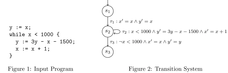
SMT solvers are a crucial tool for automated reasoning. For instance, consider the example program in Figure1 and its translation into an integer transition system in Figure 2. In the latter, a primed variablex0 represents the value ofxafter the transition.
y := x;
while x < 1000 { y := 3y - x - 1500; x := x + 1;
}
Figure 1: Input Program
s1
s2
s3
τ1:x0=x∧y0=x
τ2:x <1000∧y0= 3y−x−1500∧x0=x+ 1
τ3:¬x <1000∧x0=x∧y0=y
Figure 2: Transition System
In order to prove that a certain property is satisfied at the end of the program, one can determine invariants of each state and then show their validity. For instance, for ensuring that y ≤xholds at the end of the program, one can show that y ≤x is an invariant of states s2
and s3. Verifying these invariants amounts to checking the validity of formulas (1)–(3), each
corresponding to one transition.
τ1−→y0≤x0 (1)
y≤x∧τ2−→y0≤x0 (2)
y≤x∧τ3−→y0≤x0 (3)
are valid, expressing the decrease of the ranking function (4) and its boundedness (5).
τ2−→(1000−x)>(1000−x0) (4)
τ2−→(1000−x0)≥0 (5)
So, verifying soundness properties and termination proofs of programs can be performed via validity checking of formulas, or equivalently, by checking unsatisfiability of the negated formulas, which can easily be done by invoking an SMT solver.
There is one problem though: since SMT solvers are complex pieces of software, they might contain errors and therefore wrongly detect unsatisfiability of a formula. To solve this problem, there are in principle two approaches.
1. One can use a certificate emitting SMT solver and check the validity of each generated certificate by a verified certificate checker.
2. One can directly develop a verified SMT solver.
The two approaches are mutually incomparable.
Approach1has the advantage that it is much simpler to verify a certificate checker than to verify a full SMT solver. Moreover, this approach will usually be more efficient, since one can profit from all the (unverified) optimizations that will speed up the proof search in the SMT solver, so that only the final proof has to be checked by the verified certificate checker.
Approach 2 on the other hand has the advantage, that it is easier to use: one just has to install one program and there is no risk that there is a synchronization problem, where the SMT solver and certifier disagree on the format or meaning of the certificate.
CeTA is a verified certificate checker for program properties and especially for termination proofs. In particular, it can take the above transition system from Figure2 as input in com-bination with the set of invariants, or the ranking function or a more complex termination proof [BJTY17]. Internally, it will create the formulas as illustrated and check the validity of the invariants or of the ranking function. The soundness of CeTA has been formally verified in Isabelle/HOL, i.e., if it accepts a set of invariants then they are indeed valid invariants, and an accepted ranking function will indeed prove termination. When it comes to checking unsatisfiability of a formula,CeTAcurrently offers both approaches.
In Approach1, one has to provide a list of Farkas coefficients from the SMT solver to prove unsatisfiability.2 For instance, the negation of formula (2) is
y ≤x∧x <1000∧y0 = 3y−x−1500∧x0=x+ 1∧y0> x0 (6) which can equivalently be written as the set of non-strict linear inequalities (7)–(13).
−x+ y ≤0 (7)
x ≤999 (8)
−x+ 3y − y0≤1500 (9)
x− 3y + y0≤ −1500 (10)
x −x0 ≤ −1 (11)
−x +x0 ≤1 (12)
x0− y0≤ −1 (13)
2CeTAdoes not invoke an external SMT solver to obtain these coefficients on its own, they have to be part
The Farkas coefficients in the certificate (3, 1, 0, 1, 1, 0, 1) tell us how to add and multiply each equation. In the example, computing
3·(7) + 1·(8) + 0·(9) + 1·(10) + 1·(11) + 0·(12) + 1·(13)
we arrive at the inequality 0 ≤ −503, which directly proves the unsatisfiability of (6) and therefore the validity of (2). The problem here is the synchronization between the coefficients in the certificate and the formula: what is the order of linear inequalities (7)–(13), what is the order of the formulas (1)–(3), etc.? This problem manifested during the integration of the termination analyzer T2 and the certifier CeTA. To be more precise, complex proofs of
T2 had to be validated by CeTA, where the proofs of T2 contained several validity claims of formulas, and where most of these formulas are not explicitly spelled out in the certificate, but are automatically generated from stated invariants, ranking functions, transition formulas, etc. Overall, it took several iterations of modifying bothT2andCeTAuntil the precise order of formulas and Farkas coefficients had been synchronized.
This synchronization problem is not at all present in Approach 2, where CeTA needs no additional information in the certificate to check the validity of formulas, and just invokes its basic verified SMT solver in order to prove that (6) and other formulas are unsatisfiable. For instance, the termination analyserAProVEdoes not provide Farkas coefficients in the certificate and solely relies uponCeTA’s internal SMT solver for checking its proofs.
In total, both approaches pose some problems: an engineering problem to synchronize certifi-cates in Approach1, and a verification problem to obtain a verified SMT solver in Approach2. In the remainder of this paper we will only consider Approach 2, i.e., we are interested in developing an efficient verified SMT solver.
3
Existing Simplex Formalization
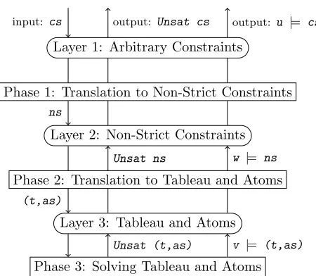
The simplex algorithm as described by Dutertre and de Moura works in several phases as illustrated in Figure3.
First, in Phase 1 the input constraints are transformed from arbitrary linear (in)equalities (Layer 1) into a set of non-strict inequalities (Layer 2). Next, in Phase 2 these constraints are translated into a tableau—a set of linear equations having a specific shape—in combination with atoms of the form x ≤ c or x ≥ c for variables x and constants c (Layer 3). Then in Phase 3 the tableau, the atoms and a valuation are modified until a solution or unsatisfiability is detected. These modifications in Phase 3 can be done incrementally: by asserting a new atom; by performing cheap, but incomplete deduction; or by a full satisfiability test using pivoting. Finally, unsatisfiability in Layer 3 is propagated upwards to Layer 1, and a satisfying valuation of Layer 3 is transformed into a satisfying valuation of Layer 1 by passing Phases 2 and 1 again. Spasi´c and Mari´c formalized most of this algorithm in a modular style via several refine-ment steps. Specifically, they define several specifications in the form of locales [Bal14] that describe the required behavior for the individual layers and phases. A locale can demand cer-tain functions viafixes that satisfy several conditions specified byassumes. For instance, their specification on Layer 1 is formulated in the locale with nameSolve. It postulates a function
solve of a type which takes a constraint list as input and returns an option type. The result
None represents unsatisfiability, and if some valuation v is returned, then this must be a sat-isfying valuation. Here, the relation|=cs encodes whether a given valuation satisfies a set of constraints.3
3We identify lists and sets throughout this paper, whereas in the formalization an explicit conversion is
Layer 1: Arbitrary Constraints
Phase 1: Translation to Non-Strict Constraints
Layer 2: Non-Strict Constraints
Phase 2: Translation to Tableau and Atoms
Layer 3: Tableau and Atoms
Phase 3: Solving Tableau and Atoms
input: cs
ns
(t,as)
Unsat (t,as) Unsat ns output:Unsat cs
v |= (t,as)
w |= ns
output: u |= cs
Figure 3: The Layers and Phases of the Simplex Algorithm
locale Solve =
fixes solve :: constraint list ⇒ rat valuation option assumes solve cs = None =⇒ ¬ (∃ v. v |=cs cs)
and solve cs = Some v =⇒ v |=cs cs
A very similar specification is provided on Layer 2 for non-strict inequalities via the locale
Solve_Ns. Here, |=ns is like |=cs, only the type of constraints is changed from arbitrary to
non-strict constraints, and the domain is changed from rational numbers to some type α of classlrv, representing linearly ordered rational vectors.
locale Solve_Ns =
fixes solve_ns :: α ns_constraint list ⇒ α valuation option assumes solve_ns cs = None =⇒ ¬ (∃ v. v |=ns cs)
and solve_ns cs = Some v =⇒ v |=ns cs
The transition between these two specifications, Phase 1, is again just an abstract specifica-tion. It demands a translationto_ns from arbitrary to non-strict constraints so that they are equisatisfiable. The translationto_ns will be used for the left path in Figure3. Moreover, also a computable translationfrom_ns is required. It converts a satisfying valuation of the non-strict constraints into a satisfying valuation of the input constraints, corresponding to the right path in Figure3.
locale To_Ns =
fixes to_ns :: constraint list ⇒ α ns_constraint list
and from_ns :: α valuation ⇒ α ns_constraint list ⇒ rat valuation
assumes v |=cs cs =⇒ ∃ w. w |=ns to_ns cs
and w |=ns to_ns cs =⇒ from_ns w (to_ns cs) |=cs cs
locale Solve_Ns0 = Solve_Ns solve_ns + To_Ns to_ns from_ns begin
definition solve_impl cs = let
ns_cs = to_ns cs
in case solve_ns ns_cs of
None ⇒ None
| Some w ⇒ Some (from_ns w ns_cs)
sublocale Solve solve_impl
end
In the locale, the line starting with sublocale states that solve_impl satisfies the speci-fication of the locale Solve. The formalization also contains the corresponding proof of this statement.
Afterwards, the formalization continues to provide an implementation of To_Ns (Phase 1), and the implementation of Solve_Ns, i.e., a solver for Layer 2. Both of these tasks can be performed completely independently. The latter task is then split again into a specification and implementation of Phase 2 as well as specification and implementation of a solver for Layer 3. This solver is then further split into operations like pivoting, asserting atoms, etc.
So, the overall formalization consists of several specifications, targeting the different phases and layers. And the overall algorithm is composed by refining several (small) specifications by verified implementations. Plugging together all the individual algorithms is then an easy task, since soundness is automatically obtained via the locale structure.
4
New Simplex Formalization
In the following we describe our extension of the formalization of Spasi´c and Mari´c by the integration of unsatisfiable cores (Section4.1) and the development of an incremental interface to the simplex algorithm (Section4.2).
4.1
Unsatisfiable Cores
Our first extension is the integration of an unsatisfiable core, i.e., given a set of unsatisfiable constraints, we are interested in a subset of the constraints which is still unsatisfiable. Small unsatisfiable cores are crucial for a DPLL(T) based SMT solver in order to derive small conflict clauses. For example, already the subset (7,8,10,11,13) of the constraints (7–13) is unsatisfiable. The first question for our extension is about the representation of unsatisfiable cores. Clearly, one has to change the return types of the solvers at the various layers—currentlyα valuation
option—to a sum typeβ + valuationwhereβ is some type that represents unsatisfiable cores.
at this point, i.e., constraints (or atoms) became pairs of an index and the actual constraint (or atom). However, the equations in the tableau do not need any indices since these are global, i.e., the same equations will be used for every subset of the constraints (or atoms).
In general, we adapted the formalization in a controlled way, i.e., we made several small changes to it, so that after each change all proofs are still accepted by Isabelle.
The first change was the modification of the return type of the solvers and the switch to indexed constraints and atoms (i_constraint, i_ns_constraint, etc.) for the input. Here, the implementation just passes the indices around. For example, where before an arbitrary con-straintcwas translated into a set of non-strict constraintsns, now an indexed constraints (i, c) is translated into{(i, n)| n ∈ns}. And whenever unsatisfiability is detected, the implemen-tation now returns∅as an unsatisfiable core instead of just stating unsatisfiability. Of course, the empty set is not an unsatisfiable core, but this is not a problem: the specifications of all layers ignore the core and also all indices are ignored via the functionflat, which just removes all indices from indexed constraints and atoms. In this way, the introduction of indices and the change of the return type to an unsatisfiable core is not that big.
As a concrete example, in the first change we modified the localeSolve_Ns to the following one whereInl andInr are the constructors of Isabelle’s sum-type, andι is the type of indices. We use the letterI to abbreviate a list or set of indices.
locale Solve_Ns =
fixes solve_ns :: (ι, α) i_ns_constraint list ⇒ ι list + α valuation
assumes solve_ns cs = Inl I =⇒ ¬ (∃ v. v |=ns flat cs) (* ignore indices and I *)
and solve_ns cs = Inr v =⇒ v |=ns flat cs (* ignore indices *)
The next change was the modification of the specifications of all layers like Solve, Solve_ Ns, etc., so that a returned set of indices can be guaranteed to be an unsatisfiable core. The implementation was easily changed to meet these specifications by just always returning the set of all indices in case of unsatisfiability. Note that at this step we do not modify the specifications of any of the phases likeTo_Ns.
As an example, the locale Solve is changed into the following one where |=ics and |=ins are the indexed versions of|=cs and |=ns, e.g., (I,v) |=ics cs if and only ifI |=cs {c|(i,c)∈
cs∧i∈I}.
locale Solve =
fixes solve :: ι i_constraint list ⇒ ι list + rat valuation
assumes solve cs = Inl I =⇒ ¬ (∃ v. (I,v) |=ics cs) (* new *)
and solve cs = Inr v =⇒ v |=ns flat cs
Moreover, the definition of the implementationsolve_impl is changed as follows wheremap
fst cs encodes the set of all indices.
definition solve_impl cs = let
ns_cs = to_ns cs
in case solve_ns ns_cs of
Inl I ⇒ Inl (map fst cs) (* new *)
| Some w ⇒ Some (from_ns w ns_cs)
of Spasi´c and Mari´c includes neither unsatisfiable cores nor a notion of satisfiability of indexed constraints.
The final step consisted of a sequence of modifications. Each of these treated one particular phase of the simplex algorithm. For instance, in Phase 1, we strengthened the specification in one direction to indexed subsets.
locale To_Ns =
fixes to_ns :: i_constraint list ⇒ α i_ns_constraint list
and from_ns :: α valuation ⇒ α ns_constraint list ⇒ rat valuation
assumes (I,v) |=ics cs =⇒ ∃ w. (I,w) |=ins to_ns cs (* new *)
and w |=ns flat (to_ns cs) =⇒ from_ns w (flat (to_ns cs)) |=cs flat cs
With the modified localeTo_Ns one can easily prove soundness of the final version ofsolve_ impl. Instead of always returning the full set of indices, the final version just propagates the set of indices: the previous lineInl I ⇒ Inl (map fst cs)on page43is replaced byInl I ⇒
Inl I.
The main work w.r.t. the modification of the transition to non-strict constraints is proving that the implementation of To_Ns still satisfies the strengthened specification. The existing proof only contains the result that the new condition is satisfied wheneverI is the set of all indices. We do not provide further details at this point, but just state that these generalizations of the proofs were of different difficulty levels.
• The generalizations for Phases 1 and 2 were rather straight-forward.
• The algorithms of Phase 3 which initially detect unsatisfiability required most adaptations and some new proofs.
• One of the most complex operations in the simplex algorithm in Phase 3, pivoting, luckily required hardly any changes: since pivoting only changes the tableau and since the tableau has no indices, there was not much to adapt. Here, the modular design of Spasi´c and Mari´c was clearly helpful, which separates pivoting via its own abstract specification.
After all these modifications we obtain an implementation that meets the specification of
Solve on page43. The implementation indeed returns non-trivial unsatisfiable cores, e.g., it
computes (7,8,10,11,13) as unsatisfiable core of (7–13).
The formalization for Isabelle 2018 does not contain proofs of the minimality of the unsatis-fiable cores. But motivated by a reviewer comment, we started to investigate minimality of the cores. We soonish detected two side-conditions on the inputs which are essential for obtaining minimal cores, cf. Example1.
Example 1. Consider the following indexed constraints [(A, x ≤3),(B, x ≤5),(B, x ≥10)] where some index (B) refers to two different constraints. If we invoke the verified simplex algorithm on these constraints, it will detect that x ≤ 3 is in conflict to x ≥ 10 and hence produce {A, B} as unsatisfiable core. This core is clearly not minimal since {B} is already unsatisfiable.
We show that the problems in Example 1 are the only ones which prohibit the generation of a minimal unsatisfiable core. In a more recent version of the formalization (AFP revision dd35fc1288c14) we proved minimality of the unsatisfiable cores for all layers under mild pre-conditions: On Layer 3 the tableau must not contain any equation of the formx= 0, and all indices in the atoms must be distinct. In order to satisfy these preconditions of Layer 3, we demand in Layer 2 that the indices of the non-strict constraints are distinct, and that there is no ground constraint 0 ≤c or 0 ≥c for a constantc. Finally, on Layer 1 we again demand distinctness of the indices and we forbid ground constraints and equality constraints. The lat-ter are problematic since each indexed equality constraint will be translated into two non-strict inequalities that share the same index and therefore violate distinctness of indices on Layer 2.
Interestingly, the integration of minimal unsatisfiable cores required us to modify the locale structure. For instance, the locale for asserting a new atom was previously completely inde-pendent from the pivoting operation. In contrast, now pivoting is used for proving that each proper subset of an unsatisfiable core is satisfiable, whenever the assertion operation detects unsatisfiability.
4.2
Incremental Simplex
The specification Solve is monolithic: one has to invoke the function solve on every new input so that the computation will start from scratch, even if two inputs differ only in a single constraint. Hence, the existing formalization of Spasi´c and Mari´c definitely does not specify an incremental simplex algorithm, despite the fact that some sub-algorithms of Phase 3 provide an incremental interface.
Since incrementality of a theory solver is a crucial requirement for developing a DPLL(T) based SMT solver, the second big modification is to make the existing simplex formalization incremental at each layer. For the exact incremental interface, we closely follow Dutertre and de Moura who propose the following operations.
• Initialize the solver by providing the set of all possible constraints. This will return a state where none of these constraints has been asserted.
• Assert a constraint. This invokes a computationally inexpensive deduction algorithm and returns an unsatisfiable core or a new state.
• Check a state. Perform an extensive deduction algorithm that decides satisfiability of the set of asserted constraints. It returns an unsatisfiable core or a checked state.
• Extract a solution of a checked state.
• Compute some checkpoint information of a checked state.
• Backtrack to a state with the help of some checkpoint information.
In Isabelle we specify this informal interface for Layer 1 in the localeIncremental_Simplex_ Ops where the type-variableσrepresents the state andγ is the checkpoint information.
locale Incremental_Simplex_Ops =
fixes init :: ι i_constraint list ⇒ σ
and assert :: ι ⇒ σ ⇒ ι list + σ
and check :: σ ⇒ ι list + σ
and solution :: σ ⇒ (var, rat) mapping
and checkpoint :: σ ⇒ γ
and backtrack :: γ ⇒ σ ⇒ σ
and invariant :: ι i_constraint list ⇒ ι set ⇒ σ ⇒ bool
and checked :: ι i_constraint list ⇒ ι set ⇒ σ ⇒ bool
assumes checked cs {} (init cs)
and checked cs J s =⇒ invariant cs J s
and invariant cs J s =⇒ assert j s = Inr s0 =⇒ invariant cs ({j} ∪ J) s0
and invariant cs J s =⇒ assert j s = Inl I =⇒ I ⊆ {j} ∪ J ∧ @ v. (I, v) |=ics cs
and invariant cs J s =⇒ check s = Inr s0 =⇒ checked cs J s0
and invariant cs J s =⇒ check s = Inl I =⇒ I ⊆ J ∧ @ v. (I, v) |=ics cs
and checked cs J s =⇒ solution s = v =⇒ (J, v) |=ics cs
and checked cs J s =⇒ checkpoint s = c =⇒ invariant cs K s0 =⇒
backtrack c s0 = s00 =⇒ J ⊆ K =⇒ invariant cs J s00
The interface consists of the six operations init, . . . , backtrack to invoke the algorithm, and the two invariantsinvariant and checked, where the latter entails the former.
Both invariants take the same list of argumentsinvariant cs I sandchecked cs I s. Here, cs is the global set of indexed constraints that is encoded in state s. It can only be set by
invokinginit cs and is kept constant otherwise. The parameterI indicates the subset of all constraints that has been asserted in states.
We shortly explain the specification of assert and backtrack and leave the usage of the remaining functionality to the reader.
For theassert operation there are two outcomes. If the assertion of indexj was successful and delivers a new state s0 then the newly asserted set of constraints is indeed increased by precisely the indexj. Otherwise, the operation returns some unsatisfiable set of indicesI such thatI is a subset of everything that has been asserted, includingj, and the set of allI-indexed constraints is unsatisfiable.
The backtracking facility works as follows. Assume one has computed the checkpoint infor-mationc in states, which is only permitted ifs satisfies the stronger invariant for some set of
indicesJ. Afterwards, one may have performed arbitrary operations to switch to states0which
corresponds to a superset of indicesK⊇J. Then purely froms0 andc one can compute a new states00viabacktrackthat corresponds to the old set of indicesJ. Of course, the implementa-tion should be done in a way thatcis small in comparison tos, so in particularc should not be
s itself. And indeed our implementation behaves in the same way as the informally described algorithm by Dutertre and de Moura: for a checkpoint we store (indexed) atoms, but not the tableau.
In order to implement the incremental interface, we took the same approach as Spasi´c and Mari´c. We began by constructing specifications likeIncremental_Simplex_Ops for the other two layers. Next, in order to implement some layer, we tried to use the existing functionality of the various phases which often required further generalizations.
For instance, the operations of Phase 3 could mostly be taken from the existing formalization, but a few generalizations w.r.t. indexed atoms had to be integrated. Similarly, Phase 1 requires another generalization in the localeTo_Ns: now, both directions enforce indexed variants.
locale To_Ns =
and from_ns :: α valuation ⇒ α ns_constraint list ⇒ rat valuation assumes (I,v) |=ics cs =⇒ ∃ w. (I,w) |=ins to_ns cs
and (I,w) |=ins to_ns cs =⇒ (I,from_ns w (flat (to_ns cs))) |=ics (I,cs) (* new *)
Interestingly, in the translation of a satisfying assignment via from_ns, it is not required
to first filtercs to those constraints that have an index fromI because of some newly proven monotonicity property. The benefit of not having to filter can then be exploited in the im-plementation. In the verified algorithm, the previously computed non-strict constraints to_
ns cs are reused, whenever a satisfying assignment needs to be converted viafrom_ns.
As final result of our formalization, we combine the implementations of all phases and layers to obtain a fully verified implementation of the simplex algorithm w.r.t. the specification defined in the localeIncremental_Simplex_Ops.
5
Conclusion
We developed an Isabelle/HOL formalization of an incremental simplex algorithm with unsat-isfiable core generation.
It is mainly an extension of the simplex formalization of Spasi´c and Mari´c. The modular structure of their proof was clearly beneficial. It supported a step-by-step integration of the required changes to provide unsatisfiable cores. In particular, we did not have to touch the pivoting function, one of the most complex operations of the existing formalization. However, the refinement approach of the existing formalization was also sometimes cumbersome. Since the top-level specification was non-incremental and did not include unsatisfiable cores, we had to integrate these features into several layers of the refinement.
The new incremental simplex formalization is only a stepping stone towards our initial goal, the development of a verified SMT solver that is based on the DPLL(T) approach. It remains to figure out if and how it can be coupled with the existing DPLL based verified SAT solver [BFLW18]. Moreover, our current simplex algorithm only supports the theory of LRA. Here, the integration of techniques like branch and bound or Gomory cuts would be interesting for the support of LIA, or, more generally, mixed integer problems [DdM06, Chapter 4 of Technical Report]. In order to formally prove termination, a recent transformation [Bro18] might be useful which turns arbitrary mixed integer problems into bounded ones.
Acknowledgments
This research was supported by the Austrian Science Fund (FWF) project Y757. We thank Ralph Bottesch, Max W. Haslbeck and the anonymous reviewers for their helpful comments.
References
[Bal14] Clemens Ballarin. Locales: A module system for mathematical theories. J. Autom. Rea-soning, 52(2):123–153, 2014.
[BCI+16] Marc Brockschmidt, Byron Cook, Samin Ishtiaq, Heidy Khlaaf, and Nir Piterman. T2: Temporal property verification. In Marsha Chechik and Jean-Fran¸cois Raskin, editors,
[BFLW18] Jasmin Christian Blanchette, Mathias Fleury, Peter Lammich, and Christoph Weidenbach. A verified SAT solver framework with learn, forget, restart, and incrementality. J. Autom. Reasoning, 61(1-4):333–365, 2018.
[BGS18] Maria Paola Bonacina, St´ephane Graham-Lengrand, and Natarajan Shankar. Proofs in conflict-driven theory combination. In June Andronick and Amy P. Felty, editors, Proceed-ings of the 7th ACM SIGPLAN International Conference on Certified Programs and Proofs, CPP 2018, Los Angeles, CA, USA, January 8-9, 2018, pages 186–200. ACM, 2018. [BJTY17] Marc Brockschmidt, Sebastiaan J. C. Joosten, Ren´e Thiemann, and Akihisa Yamada.
Cer-tifying safety and termination proofs for integer transition systems. In Leonardo de Moura, editor, Proceedings of the 26th International Conference on Automated Deduction (CADE 2017), volume 10395 ofLecture Notes in Computer Science, pages 454–471. Springer, 2017. [Bro18] Martin Bromberger. A reduction from unbounded linear mixed arithmetic problems into bounded problems. In Didier Galmiche, Stephan Schulz, and Roberto Sebastiani, editors,
Automated Reasoning, 9th International Joint Conference, IJCAR 2018, Oxford, UK, July 14-17, 2018, Proceedings, volume 10900 ofLecture Notes in Computer Science, pages 329– 345. Springer, 2018.
[CS01] Michael Col´on and Henny Sipma. Synthesis of linear ranking functions. In Tiziana Margaria and Wang Yi, editors,Tools and Algorithms for the Construction and Analysis of Systems, 7th International Conference, TACAS 2001, Genova, Italy, April 2-6, 2001, Proceedings, volume 2031 ofLecture Notes in Computer Science, pages 67–81. Springer, 2001.
[DdM06] Bruno Dutertre and Leonardo Mendon¸ca de Moura. A fast linear-arithmetic solver for DPLL(T). In Thomas Ball and Robert B. Jones, editors,Computer Aided Verification, 18th International Conference, CAV 2006, Seattle, WA, USA, August 17-20, 2006, Proceedings, volume 4144 ofLecture Notes in Computer Science, pages 81–94. Springer, 2006. Extended version available as Technical Report, CSL-06-01, SRI International.
[GAB+17] J. Giesl, C. Aschermann, M. Brockschmidt, F. Emmes, F. Frohn, C. Fuhs, J. Hensel, C. Otto, M. Pl¨ucker, P. Schneider-Kamp, T. Str¨oder, S. Swiderski, and R. Thiemann. Analyzing program termination and complexity automatically with AProVE. J. Autom. Reasoning, 58:3–31, 2017.
[GHN+04] Harald Ganzinger, George Hagen, Robert Nieuwenhuis, Albert Oliveras, and Cesare Tinelli. DPLL(T): Fast decision procedures. In Rajeev Alur and Doron A. Peled, editors,Computer Aided Verification, 16th International Conference, CAV 2004, Boston, MA, USA, July 13-17, 2004, Proceedings, volume 3114 ofLecture Notes in Computer Science, pages 175–188. Springer, 2004.
[MST18] Filip Mari´c, Mirko Spasi´c, and Ren´e Thiemann. An incremental simplex algorithm with unsatisfiable core generation. Archive of Formal Proofs, August 2018. http://isa-afp. org/entries/Simplex.html, Formal proof development.
[NPW02] Tobias Nipkow, Lawrence C. Paulson, and Markus Wenzel. Isabelle/HOL – A Proof Assis-tant for Higher-Order Logic, volume 2283 ofLecture Notes in Computer Science. Springer, 2002.