Vol. 4, No. 3, Year 2012 Article ID IJIM-00225, 10 pages Research Article
Developing a Data Envelopment Analysis
Methodology for Supplier Selection in the
Presence of Fuzzy Undesirable Factors
N. Ahmadya∗, E. Ahmadyb, S. A. H. Sadeghib
(a)Department of Mathematics, Varamin-Pishva Branch, Islamic Azad University, Varamin, Iran. (b)Department of Mathematics, Shahr-e-Qods Branch, Islamic Azad University, Tehran, Iran.
—————————————————————————————————— Abstract
Supplier selection is a multi-criteria decision problem which includes both qualitative and quantitative factors. We present in this paper a model for supplier selection based on DEA methodology that considered both undesirable factors and fuzzy data simultaneously. The proposed method has been illustrated by a numerical example.
Keywords : Data envelopment analysis; Supplier selection; Undesirable factors; Fuzzy data.
——————————————————————————————————
1
Introduction
Nowadays fierce competitive environment, characterized by thin profit margins, high con-sumer expectations for quality products and short lead-times, companies are forced to take advantage of any opportunity to optimize their business processes. To reach this aim, academics and practitioners have come to the same conclusion: for a company to remain competitive, it has to work with its supply chain partners to improve the chain’s total performance. Thus, being the main process in the upstream chain and affecting all areas of an organization. Purchasing is one of the most important strategic activities in supply chain [1]. One of the most critical functions in purchasing is to select supplier. The objective of supplier selection process is to identify suppliers with the highest poten-tial for meeting a manufacturer’s needs consistently and acceptable overall performance. Selecting suppliers from a large number of possible suppliers with various levels of ca-pabilities and potential is a difficult task and inherently a multi criteria decision-making
∗Corresponding author. Email address: [email protected]
(MCDM) problem. Supplier selection decisions are complicated because various criteria must be considered in the decision-making process [2, 5, 7]. One of the techniques for supplier selection is Data Envelopment Analysis (DEA). Data envelopment analysis mea-sures the relative efficiency of decision making units (DMUs) with multiple performance factors which are grouped into outputs and inputs. Once DEA identifies the efficient fron-tier, DEA improves the performance of inefficient DMUs by either increasing the current output levels or decreasing the current input levels [8]. However, both desirable and un-desirable output and input factors may be present. However, in the standard DEA model, decreases in outputs are not allowed and only inputs are allowed to decrease. (Similarly, increases in inputs are not allowed and only outputs are allowed to increase). For example, if inefficiency exists in production processes where final products are manufactured with a production of wastes and pollutants, the outputs of wastes and pollutants are undesirable and should be reduced to improve the performance[9].Traditional DEA models do not deal with imprecise data and assume that all input and output data are exactly know, but in real world, this assumption is not always true. Uncertain information or imprecise data can be expressed in interval or fuzzy number. In many real-world applications DEA (especially supplier selection problems), it is essential to take into account the existence of both undesirable factors and both qualitative and quantitative factors. This paper de-picts the supplier selection process through an fuzzy data envelopment analysis (FDEA) model, while allowing for the incorporation of undesirable factors. The aim of this paper is to propose a data envelopment analysis models for selecting the best suppliers in the presence of both undesirable factors and fuzzy data. The proposed approach developed in this paper includes a number of contributions, as follows:
- This paper proposed a model capable of treating imprecise factors.
-The proposed model considers multiple criteria, this helps managers to select suppliers using a comprehensive approach that goes beyond just purchase costs.
- The proposed model does not demand weights from the decision maker.
- The proposed model can consider both fuzzy data and undesirable factors for supplier selection problems.
This paper proceeds as follows. In Section 2, Notations and definitions is presented. Sec-tion 3, introduces the model, numerical example and concluding remarks are discussed in Sections 4 and 5, respectively.
2
Notation and Definition
First, the notations which shall be used in this paper will be introduced. All fuzzy sets are fuzzy subsets of real numbers. A fuzzy number is a fuzzy set of the real line with a normal, convex and upper semicontinuous membership function of a bounded support. The family of fuzzy numbers will be denoted by E .The membership function for fuzzy number u can be expressed as
u(x) =
ul(x), a≤x≤b,
1, b≤x≤c, ur(x), c≤x≤d,
0 otherwise.
(2.1)
Where ul: [a, b]→[0,1] andur: [a, b]→[0,1] are left and right membership functions of
Definition 2.1. An arbitrary fuzzy number is presented by an ordered pair of functions
(u(α), u(α)),0≤α≤1 , which satisfies the following requirements:
1-u(α) is a bounded left continuous nondecreasing function over [0,1], with respect to any
α.
2-u(α) is a bounded left continuous nonincreasing function over [0,1], with respect to any
α.
3-u(α)≤u(α),0≤α≤1.
The trapezoidal fuzzy number u = (x0, y0, s, t) with two defuzzifier x0, y0 and left
fuzziness s > 0 and right fuzziness t >0 is a fuzzy set where the membership function is as
u(x) =
1
s(x−x0+s) x0−s≤x≤x0
1 x∈[x0, y0] 1
t(y0−x+t) y0 ≤x≤y0+t
0 otherwise.
(2.2)
and parametric form is
u(α) =x0−s+sα, u(α) =y0+t−tα.
Definition 2.2. For arbitrary u = (u(α), u(α)), v = (v(α), v(α)) and k > 0, addition, standard substraction and standard multiplication by k are as follows:
u+v= (u(α) +v(α), u(α) +v(α))
u−v= (u(α)−v(α), u(α)−v(α))
ku=
{
(ku, ku) if k≥0,
(ku, ku) if k <0. (2.3) Definition 2.3. [6] For arbitrary fuzzy numbersu = (u(α), u(α)) and v = (v(α), v(α)), the function
dp(u, v) = [
∫ 1
0
|u(α)−v(α)|pdr+
∫ 1
0
|u(α)−v(α)|pdα]1/p (p≥1) (2.4)
is the distance between u andv.
Definition 2.4. [3]Let{A1, A2,· · ·, Am} are m numbers, the Maximizing set M is fuzzy
subset with membership function M(x) given as
M(x) =
{
[ (x−xmin) (xmax−xmin)]
k, x
min ≤x≤xmax,
0, otherwise, (2.5)
where xmin= infS, xmax = supS, S=
∪n
i=1Si, andSi ={x|Ai(x)>0}.
Definition 2.5. [3] Let{A1, A2,· · ·, Am} are m numbers, the Minimizing set Gis fuzzy
subset with membership function G(x) given as
G(x) =
{
[ (x−xmax) (xmax−xmin)]
k, x
min≤x≤xmax,
0, otherwise, (2.6)
where xmin= infS, xmax = supS, S=
∪n
Figure 1: The maximizing set for fuzzy numbersA1,A2 andA3.
3
Proposed approach
Consider a situation where n members of a set of nDMUs are to be evaluated in terms of s fuzzy outputs Yk = (yrk)sr=1 and m fuzzy inputs Xk = (xik)mi=1, where Y
(D)
k =
(y(rkD))s1
r=1 andY (U)
k = (−y
(U)
rk ) s2 r=1= (yb
(U)
rk ) s2
r=1are desirable and undesirable fuzzy outputs,
Xk(D) = (x(ikD))m1
i=1 and X (U)
k = (x
(U)
ik ) m2
i=1 are desirable and undesirable fuzzy inputs, in
which s1+s2=s andm1+m2 =m.
3.1 Undesirable output
In this section, we consider the DEA efficiency analysis, when undesirable outputs are produced in production process. Let Yk(D) = (yrk(D))s1
r=1 andY (U)
k = (y
(U)
rk ) s2
r=1 are desirable
and undesirable fuzzy outputs, where s1 +s2 = s. In order to improved the relative
performance, we would like to increase Y(D) and on the contrary Y(U) does not allow to increase, and we would like to decrease Y(U).
For this purpose, we define maximizing set M1 for desirable outputs and maximizing set
M2 for undesirable outputs .
Let Srk=supp{yrk(D), r= 1,· · ·, s1},Srk′ =supp{−yrk(U), r= 1,· · · , s2}
Sk =
∪s1
r=1Srk, Sk′ =
∪s2 r=1Srk′ ,
xmin= infSk, xmax = supSk,and x′min = infSk′, x′max= supSk′.
Then we define minimizing setm1 for desirable set and minimizing setm2 for undesirable
set as follows:
m1(x) = {
(xmax−x)
(xmax−xmin), xmin≤x≤xmax,
0, otherwise, (3.7)
m2(x) =
{ (x′ max−x) (x′max−x′min), x
′
min≤x≤x′max,
0, otherwise, (3.8)
Also
m1(α) = (xmin, xmax−α(xmax−xmin)) (3.9)
m2(α) = (x′min, xmax′ −α(xmax−xmin)) (3.10)
The distance between YD and minimizing set m1 is shown by d(YD, m1) and is defined
as follows:
d(YkD, m1) = ( ∫ 1
0
[(m1(α)−YkD(α))2+ (m1(α)−YkD(α))2]dα) 1
2, r= 1,· · ·, s1. (3.11)
Obviously, in order to improve the relative performance, we would like to increase the distance between YkD and the worse case of yDrk,r = 1, . . . , s1.
The distance betweenYU and minimizing setm2 is shown byd(YU, m2) and is defined as
follows:
d(YkU, m2) = ( ∫ 1
0
[(m2(α)−YkU(α))2+ (m2(α)−YkU(α))2]dα) 1
2, r = 1,· · · , s2. (3.12)
In order to improve the relative performance, we would like to increase the distance be-tween YkU = (−yrkU)s2
Now we would like to increased(YD, m1) andd(YU, m2).
Base upon previous equations, we have the following linear program:
M ax β (3.13)
s.t.
n
∑
j=1
λjXij ≤Xip, i= 1,· · · , m,
n
∑
j=1
λjd(yDrj, m1)≥βd(yrpD, m1), r= 1,· · ·, s1,
n
∑
j=1
λjd(yUrj, m2)≥βd(yrpU, m2), r= 1,· · ·, s2,
n
∑
j=1
λj = 1,
λj ≥0, j= 1,· · · , n,
Also, if we have fuzzy inputs, the distance between fuzzy numbers Xij and 0 is used.
Finally we have the following models for fuzzy inputs and fuzzy desirable and undesirable outputs.
M ax β (3.14)
s.t.
n
∑
j=1
λjd(Xij,0)≤d(Xip,0), i= 1,· · · , m,
n
∑
j=1
λjd(yDrj, m1)≥βd(yrpD, m1), r= 1,· · ·, s1,
n
∑
j=1
λjd(yUrj, m2)≥βd(yrpU, m2), r= 1,· · ·, s2,
n
∑
j=1
λj = 1,
λj ≥0, j= 1,· · · , n,
4
Numerical example
Table 1: Depicts the supplier’s characters
Supplier Inputs Desirable output Undesirable output
No TC SR NB PPM
x1j x2j y1j y2j
1 253 (0.015 +α,0.229−α) (50 +α,65−α) (α,2−α) 2 268 (0.027 +α,0.403−α) (60 +α,70−α) (4.3 +α,6.3−α) 3 259 (0.012 +α,0.182−α) (40 +α,50−α) (3.6 +α,5.6−α) 4 180 (0.017 +α,0.256−α) (100 +α,160−α) (28 + 2α,32−2α) 5 257 (0.014 +α,0.204−α) (45 +α,55−α) (28 + 2α,32−2α) 6 248 (0.011 +α,0.163−α) (85 +α,115−α) (28 + 2α,32−2α) 7 272 (0.022 +α,0.321−α) (70 +α,95−α) (28 + 2α,32−2α) 8 330 (0.031 +α,0.452−α) (100 +α,180−α) (12.8 +α,14.8−α) 9 327 (0.024 +α,0.360−α) (90 +α,120−α) (2 + 2α,6−2α) 10 330 (0.019 +α,0.287−α) (50 +α,80−α) (29 +α,29−α) 11 321 (0.054 +α,0.797−α) (250 +α,300−α) (25.4 +α,27.4−α) 12 329 (0.043 +α,0.635−α) (100 +α,150−α) (24.8 +α,26.8−α) 13 281 (0.048 +α,0.711−α) (80 +α,120−α) (24.8 +α,26.8−α) 14 309 (0.038 +α,0.567−α) (200 +α,350−α) (20.9 +α,22.9−α) 15 291 (0.034 +α,0.506−α) (40 +α,55−α) (8 +α,10−α) 16 334 (0.061 +α,0.892−α) (75 +α,85−α) (6 +α,9−α) 17 249 (0.01 +α,0.145−α) (90 +α,180−α) (4.3 + 2α,8.3−2α) 18 216 (0.06866 +α,1) (90 +α,150−α) (27.8 +α,29.8−α)
For desirable outputs y1j we compute minimizing set m1, by m1 = (40,350−310α) and
for undesirable outputs y2j we have to compute minimizing set m2 for −y2j, in table 2,
−y2j is computed for undesirable outputs. Then m2 is compute bym2 = (−32,32α).
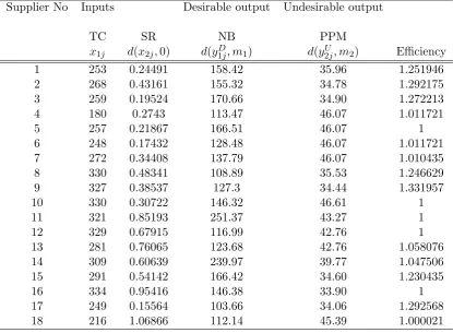
The last column of table 3, reports the results of efficiency assessments for 18 suppli-ers(DMUs) gained by using proposed model. Results of evaluation by using Model (3.14) show that, suppliers 5, 10, 11, 12, and 16 are efficient with a relative efficiency score of 1 and the remaining 13 suppliers with relative efficiency scores of more than 1 are considered to be inefficient.
5
Concluding remarks
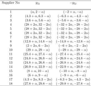
Table 2: Computing −y2j for undesirable outputs
Supplier No y2j −y2j
1 (α,2−α) (−2 +α,−α) 2 (4.3 +α,6.3−α) (−6.3 +α,−4.3−α) 3 (3.6 +α,5.6−α) (−5.6 +α,−3.6−α) 4 (28 + 2α,32−2α) (−32 + 2α,−28−2α) 5 (28 + 2α,32−2α) (−32 + 2α,−28−2α) 6 (28 + 2α,32−2α) (−32 + 2α,−28−2α) 7 (28 + 2α,32−2α) (−32 + 2α,−28−2α) 8 (12.8 +α,14.8−α) (−14.8 +α,−12.8−α) 9 (2 + 2α,6−2α) (−6 + 2α,−2−2α) 10 (29 +α,29−α) (−29 +α,−29−α) 11 (25.4 +α,27.4−α) (−27.4 +α,−25.4−α) 12 (24.8 +α,26.8−α) (−26.8 +α,−24.8−α) 13 (24.8 +α,26.8−α) (−26.8 +α,−24.8−α) 14 (20.9 +α,22.9−α) (−22.9 +α,−20.9−α) 15 (8 +α,10−α) (−10 +α,−8−α) 16 (6 +α,9−α) (−9 +α,−6−α) 17 (4.3 + 2α,8.3−2α) (−8.3 + 2α,−4.3−2α) 18 (27.8 +α,29.8−α) (−29.8 +α,−27.8−α)
Acknowledgements
Table 3: Computing distance for 18 supplier and efficiency scores
Supplier No Inputs Desirable output Undesirable output
TC SR NB PPM
x1j d(x2j,0) d(y1Dj, m1) d(y2Uj, m2) Efficiency
1 253 0.24491 158.42 35.96 1.251946 2 268 0.43161 155.32 34.78 1.292175 3 259 0.19524 170.66 34.90 1.272213 4 180 0.2743 113.47 46.07 1.011721
5 257 0.21867 166.51 46.07 1
6 248 0.17432 128.48 46.07 1.011721 7 272 0.34408 137.79 46.07 1.010435 8 330 0.48341 108.89 35.53 1.246629 9 327 0.38537 127.3 34.44 1.331957
10 330 0.30722 146.32 46.61 1
11 321 0.85193 251.37 43.27 1
12 329 0.67915 116.99 42.76 1
13 281 0.76065 123.68 42.76 1.058076 14 309 0.60639 239.97 39.77 1.047506 15 291 0.54142 166.42 34.60 1.230435
16 334 0.95416 146.38 33.90 1
References
[1] N. Aissaouia, M. Haouaria, E. Hassinib, Supplier selection and order lot sizing model-ing: A review, Computers and Operations Research 34 (2007) 3516 - 3540.
[2] C. Araz, , P. Mizrak Ozfirat, I. Ozkarahan,An integrated multi criteria decision mak-ing methodology for outsourcmak-ing management, Computers and Operations Research 34 (2007) 3738-3756.
[3] S. Chen, Ranking fuzzy numbers with maximizing set and minimizing set, Fuzzy Sets and Systems 17 (1985) 113-129.
[4] R. Farzipoor Saen, Developing a new data envelopment analysis methodology for sup-plier selection in the presence of both undesirable outputs and imprecise data, The In-ternational Journal of Advanced Manufacturing Technology 51 (2010) 1243-1250.
[5] J. Jassbi, R. Farzipoor Saen, F. Hosseinzadeh Lotfi, SH. S. Hosseininia, S. A. KHan-mohammadi,Hybrid decision-making system using data envelopment analysis and fuzzy models for supplier selection in the presence of multiple Decision makers, International Journal Of Industrial Mathematics 3 (2011) 193-212.
[6] M. Ma, M. Friedman,A. Kandel,A new fuzzy arithmetic, Fuzzy Sets and Systems 108 (1999) 83-90.
[7] M. Sanei, S. Mamizadeh Chatghaye,Evaluation of supply chain oprations using slacks-based measure of efficiency, International Journal Of Industrial Mathematics 3 (1)(2011) 35-40.
[8] L. M. Seiford, J. Zhu, Modeling undesirable factors in efficiency evaluation, European Journal of Operational Research 142(2002) 16-20.