Influence on the distribution function of annual
maximum rainfall series when filling data using
Lagrange interpolation
Arganis Juárez Maritza Liliana
1,3, Preciado Jiménez Margarita
2, Cortés Rosas
Jesús Javier
3González Cárdenas Miguel Eduardo
3, Pinilla Morán Víctor
Damián
31 Universidad Nacional Autónoma de México, Instituto de Ingeniería, Ciudad Universitaria, CDMX,
0410, México
2 Instituto Mexicano de Tecnología del Agua, Blvd. Paseo Cuauhnáhuac 8532, Jiutepec, Mor. 62550,
México
3 Universidad Nacional Autónoma de México, Facultad de Ingeniería, Ciudad Universitaria, CDMX,
0410, México
Corresponding author: [email protected]
Abstract
Lagrange interpolation was applied to complete maximum annual rainfall data for five weather stations in Aguascalientes, State of Mexico; in most of them there were no variations in the type of distribution function obtained; in general, an overestimation of the extrapolated data was identified for different return periods when the original records were not used.
Keywords: Annual maximum rainfall, Distribution function, Lagrange interpolation
1
Introduction
The calculation of the design precipitation is very important to feed rainfall runoff models with which it is possible to deliver the design flow information of a hydraulic work. The requirement for reliable information in quality and quantity motivates the use of data-filling techniques. In other studies, spatial-type interpolation techniques of precipitation data are analyzed and they would be compared at different time intervals (S. M. Vicente Serrano, 2003) (S. S. P. Shen, 2001) (T. Chen, 2017) (T. Tao, 2009). In this work the Lagrange interpolation method (Balderrama, 1990) was applied to obtain complete records of annual maximum precipitation of five climatological stations located at different points randomly in Aguascalientes State (Figure 1), in order to analyze the behavior of the distribution
Engineering
EPiC Series in Engineering
Volume 3, 2018, Pages 87–94
functions of the best fit obtained with the original data and with the records with the greatest number of data.
Figure 1: Location of climatological stations. Aguascalientes,State México
2
Methodology
2.1
Lagrange interpolation polynomial
If we have a function expressed in tabular form, in which the increase in the independent variable is not constant, i.e. it has the form:
Table 1: Example of tabular function
x x0 x1=x0+h0 x2= x1+h1 x3= x2+h2 . . xn=xn-1+hn-1
y=f(x) y0 y1 y2 y3 . . yn
where: h0=x1-x0, h1=x2-x1,. . . , hn=xn-xn-1, that means the increase in the independent variable is not
constant. The form of the polynomial that passes through n+1 points is represented as follows [4]:
𝑦 = (𝑥 − 𝑥1)(𝑥 − 𝑥2)(𝑥 − 𝑥3) … (𝑥 − 𝑥𝑛) (𝑥0− 𝑥1)(𝑥0− 𝑥2)(𝑥0− 𝑥3) … (𝑥0− 𝑥𝑛)𝑦0+
(𝑥 − 𝑥0)(𝑥 − 𝑥2)(𝑥 − 𝑥3) … (𝑥 − 𝑥𝑛)
(𝑥1− 𝑥0)(𝑥1− 𝑥2)(𝑥1− 𝑥3) … (𝑥1− 𝑥𝑛)𝑦1
+ (𝑥 − 𝑥0)(𝑥 − 𝑥1)(𝑥 − 𝑥3) … (𝑥 − 𝑥𝑛)
(𝑥2− 𝑥0)(𝑥2− 𝑥1)(𝑥2− 𝑥3) … (𝑥2− 𝑥𝑛)𝑦2+ ⋯
+ (𝑥 − 𝑥0)(𝑥 − 𝑥1)(𝑥 − 𝑥3) … (𝑥 − 𝑥𝑛−1) (𝑥𝑛− 𝑥0)(𝑥𝑛− 𝑥1)(𝑥𝑛− 𝑥3) … (𝑥𝑛− 𝑥𝑛−1)𝑦𝑛
required. In the analyzed problem the variable x is the time and the variable y is the maximum annual precipitation to be interpolated or extrapolated.
2.2
Data of climatological stations
The annual maximum precipitation data of stations 1003, 1007, 1017, 1029 and 1073, located in Aguascalientes, State México, obtained from the daily precipitation records of the CLICOM (CLImate COMputing Project) database were analyzed and refined.
2.3
Frequency Analysis of series of annual maxima
The frequencies analysis of annual maximum series is made by ordering from major to minor value of the series of length n; we estimate a period of return with empirical equations (for example Weibull's); then a parameter estimation technique is used for different probability distribution functions from which the one that reports the lowest standard error of fit is selected or the best result in the selection criterion of the distribution function.
3
Application and results
3.1
Application
of
Lagrange
interpolation
to
stations
1003,1007,1017,1029 and 1073
From the historical annual maximum precipitation data, stations id: 1003, 1007, 1017 and 1029, Lagrange polynomials of third degree were used, that is, four points were considered to perform the interpolations and precipitation polynomial was obtained it and it gave congruent results for each site; while for 1073 station we selected a polynomial of the second degree because the results were found in the missing data (on the contrary, the polynomial of the third degree gave very high values of that reported in nearby sites). Figures 2 to 6 show filled series; the historical data are highlighted with circles and interpolated data for the five stations with crossings.
Figure 3: Filled series. Interpolated data with Lagrange. Station 1007. Aguascalientes, Mexico
Figure 4: Filled series. Interpolated data with Lagrange. Station 1017. Aguascalientes, Mexico
Figure 6: Filled series. Interpolated data with Lagrange. Station 1073. Aguascalientes, México
3.2
Distribution function of the original series and the filled series
After performing the frequency analysis, the double Gumbel type was obtained as the best distribution function for both the original and the refilled series; in Figures 7 to 11 the distribution functions obtained are shown and from tables 2 to 6 we compare extrapolated design events for different return periods using the parameters of the original distribution function and the parameters of the distribution function of the series filled, with the difference in the results.
Figure 7: Distribution functions with the original series and the filled series. Station 1003
Figure 8: Distribution functions with the original series and the filled series. Station 1007
1 .0 1 1 .1 1 1 .2 5
2 5 10 20 50 100 200 500 1000 2000 5000 10000
0 50 100 150 200 250
-2 0 2 4 6 8 10
h
p
,
m
m
Z=-ln[ ln( Tr / (Tr-1) ) ] 1003 Modified data N=56 years. Duoble Gumbel
Measured (filled) Calculated
Tr, years 1 .0 1 1 .1 1 1 .2 5
2 5 10 20 50 100 200 500 1000 2000 5000 10000
0 50 100 150 200 250
-2 0 2 4 6 8 10
h
p
,
m
m
Z=-ln[ ln( Tr / (Tr-1) ) ] 1003 Original Data N=51 years. Double Gumbel
Measured Calculated Tr, years 1 .0 1 1 .1 1 1 .2 5
2 5 10 20 50 100 200 500 1000 2000 5000 10000
0 20 40 60 80 100 120 140
-2 0 2 4 6 8 10
h
p
,
m
m
Z=-ln[ ln( Tr / (Tr-1) ) ] 1007 Original Data N=38 years. Double Gumbel
Measured Calculated Tr, years 1 .0 1 1 .1 1 1 .2 5
2 5 10 20 50 100 200 500 1000 2000 5000 10000
0 20 40 60 80 100 120 140
-2 0 2 4 6 8 10
h
p
,
m
m
Z=-ln[ ln( Tr / (Tr-1) ) ] 1007 Modified data N=45 years. Double Gumbel
Measured (filled) Calculated
Figure 9: Distribution functions with the original series and the filled series. Station 1017
Figure 10: Distribution functions with the original series and the filled series. Station 1029
Figure 11: Distribution functions with the original series and the filled series. Station 1073
Table 2: Comparison of design events. Station 1003
Station 1003 Tr years 10 50 100 500 1000 10000
Original hp mm 63.91 95.34 111.13 146.59 161.62 210.98
Filled hp mm 62.71 92.59 108.13 143.01 157.74 205.67
differences hp mm 1.2 2.75 3 3.58 3.88 5.31
1 .0 1 1 .1 1 1 .2 5
2 5 10 20 50 100 200 500 1000 2000 5000 10000
0 50 100 150 200 250 300 350
-2 0 2 4 6 8 10
h
p
,
m
m
Z=-ln[ ln( Tr / (Tr-1) ) ] 1017 Modified Data N=64 years. Double Gumbel
Measured (filled) Calculated
Tr, years 1 .0 1 1 .1 1 1 .2 5
2 5 10 20 50 100 200 500 1000 2000 5000 10000
0 50 100 150 200 250 300 350
-2 0 2 4 6 8 10
h
p
,
m
m
Z=-ln[ ln( Tr / (Tr-1) ) ] 1017 Original Data N=56 years. Double Gumbel
Measured Calculated Tr, years 1 .0 1 1 .1 1 1 .2 5
2 5 10 20 50 100 200 500 1000 2000 5000 10000
0 20 40 60 80 100 120 140 160 180
-2 0 2 4 6 8 10
h
p
,
m
m
Z=-ln[ ln( Tr / (Tr-1) ) ]
1029 Original Data N=46 years. Double Gumbel
Measured Calculated Tr, years 1 .0 1 1 .1 1 1 .2 5
2 5 10 20 50 100 200 500 1000 2000 5000 10000
0 50 100 150 200 250 300
-2 0 2 4 6 8 10
h
p
,
m
m
Z=-ln[ ln( Tr / (Tr-1) ) ] 1029 Modified Data N=52 years . Double Gumbel
Measured (filled) Calculated
Tr, years 1 .0 1 1 .1 1 1 .2 5
2 5 10 20 50 100 200 500 1000 2000 5000 10000
0 20 40 60 80 100 120
-2 0 2 4 6 8 10
h
p
,
m
m
Z=-ln[ ln( Tr / (Tr-1) ) ]
1073 Modified Data N=43 years. Double Gumbel
Measured (filled) Calculated
Tr, years 1 .0 1 1 .1 1 1 .2 5
2 5 10 20 50 100 200 500 1000 2000 5000 10000
0 20 40 60 80 100 120 140
-2 0 2 4 6 8 10
h
p
,
m
m
Z=-ln[ ln( Tr / (Tr-1) ) ] 1073 Original Data N=38 years. Double Gumbel
Measured Calculated
Table 3: Comparison of design events. Station 1007
Station 1007 Tr years 10 50 100 500 1000 10000
Original hp mm 71.39 86.93 93.15 107.35 113.4 133.34
Filled hp mm 70.58 86.08 92.2 106.12 112.08 131.58
differences hp mm 0.81 0.85 0.95 1.23 1.32 1.76
Table 4: Comparison of design events. Station 1017
Station 1017 Tr years 10 50 100 500 1000 10000
Original hp mm 65.98 129.74 157.86 220.09 246.44 333.19
Filled hp mm 63.91 122.28 149.01 208.16 233.41 316.3
differences hp mm 2.07 7.46 8.85 11.93 13.03 16.89
Table 5: Comparison of design events. Station 1029
Station 1029 Tr years 10 50 100 500 1000 10000
Original hp mm 63.16 113.27 141.51 203.11 229.06 315.05
Filled hp mm 63.06 105.18 128.56 180.85 202.95 276.83
differences hp mm 0.1 8.09 12.95 22.26 26.11 38.22
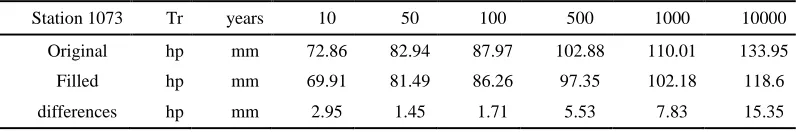
Table 6: Comparison of design events. Station 1073
Station 1073 Tr years 10 50 100 500 1000 10000
Original hp mm 72.86 82.94 87.97 102.88 110.01 133.95
Filled hp mm 69.91 81.49 86.26 97.35 102.18 118.6
differences hp mm 2.95 1.45 1.71 5.53 7.83 15.35
4
Conclusions
The Lagrange interpolation allowed to obtain series that preserved the annual historical behavior of annual maximum precipitations data in all the stations analyzed. Distribution functions are almost unaffected as a result of filling in data (interpolation). Only a slight decrease in extrapolated design precipitations was observed for different return periods when the distribution function was used with the filled series; with the exception of station 1073 where for a return period of 5 years an increase in design precipitation was observed with the series filled in, the above is attributed to the use of a second-degree polynomial for the interpolation of missing data.
5
Acknowledgments
We want to thank the DGAPA, UNAM for its support for the realization of this work within the project PAPIME PE105117 Educational Platform for Numerical Analysis
Referencias
Balderrama, R. I. (1990). Métodos Numéricos. México: First Ed. Trillas.
S. M. Vicente Serrano, M. S.-S. (2003). Comparative Analysis of Interpolation Methods in the Middle Ebro Valley (Spain). Application to annual precipitation and temperature Climate Research 24.
S. S. P. Shen, P. D. (2001). Interpolation of 1961-97 Daily Temperature and Precipitation Data onto Alberta Polygons of Ecodistrict and Soil Landscapes of Canada . Journal of Applied Meteorology 40.
T. Chen, L. R. (2017). Comparision of Spatial Interpolation Schemes for Rainfall Data and Application in Hydrological Modeling. Water 9.