Vol. 8, No. 3, 2016 Article ID IJIM-1152-00795, 8 pages Research Article
A new algorithm for solving Van der Pol equation based on piecewise
spectral Adomian decomposition method
S. Gh. Hosseini∗†, E. Babolian ‡, S. Abbasbandy§
Received Date: 2014-12-06 Revised Date: 2015-11-11 Accepted Date: 2016-02-12
————————————————————————————————–
Abstract
In this article, a new method is introduced to give approximate solution to Van der Pol equation. The proposed method is based on the combination of two different methods, the spectral Adomian decomposition method (SADM) and piecewise method, called the piecewise Adomian decomposition method (PSADM). The numerical results obtained from the proposed method show that this method is an effective, accurate and powerful tool for solving Van der Pol equation and, the comparison show that the proposed technique is in good agreement with the numerical results obtained using Runge-Kutta method. The advantage of piecewise spectral Adomian decomposition method over piecewise Adomian decomposition method is that it does not need to calculate complex integrals. Another merit of this method is that, unlike the spectral method, it does not require the solution of any linear or nonlinear system of equations. Furthermore, the proposed method is easy to implement and computationally very attractive.
Keywords: Van der Pol equation; Spectral Adomian decomposition method; Piecewise method; Runge-Kutta method.
—————————————————————————————————–
1
Introduction
M
aand engineering are related to nonlinearny problems in chemistry, biology, physics self-excited oscillators [9, 16]. The Van der Pol oscillator is a mode developed to describe the be-havior of nonlinear vacuum tube circuits in the relatively early days of the development of elec-tronics technology. Balthazar Van der Pol in-troduced his equation in order to describe tri-ode oscillations in electrical circuits[17, 6]. Van∗Corresponding author. [email protected] †Department of Mathematics, Science and Research Branch, Islamic Azad University, Tehran, Iran.
‡Department of Mathematics, Science and Research Branch, Islamic Azad University, Tehran, Iran.
§Department of Mathematics, Science and Research Branch, Islamic Azad University, Tehran, Iran.
der Pol discovered stable oscillations, now known as limit cycles, in electrical circuits employing vacuum tubes. When these circuits are driven near the limit cycle, they become entrained, i.e. the driving signal pulls the current along with it. The mathematical model for the system is a well-known second order ordinary differential equation with cubic non linearity of Van der Pol equation. Since then thousands of papers have been published attempting to achieve better ap-proximations to the solutions occurring in such non linear systems. The Van der Pol oscillator is a classical example of self-oscillatory system and is now considered as a very useful mathematical model that can be used in much more complicated and modified systems. However, this equation is so important for mathematicians, physicists and engineers to be extensively studied. The Van der
Pol equation has a long history of being used in both the physical and biological sciences. For instance, Fitzhugh [8] and Nagumo[15] used the equation in a planner field as a model for action potential of neurons. Additionally, the equation has also been extended to the Burridge–Knopoff model which characterizes earthquake faults with viscous friction[2].
During the first half of the twentieth century, Balthazar van der Pol pioneered the field of ra-dio telecommunication[4,3,18]. The Van der Pol equation with large value of nonlinearity param-eter has been studied by Cartwright and Little-wood [5]; they showed that the singular solution exists. Furthermore, analytically, Lavinson [14], analyzed the Van der Pol equation by substitut-ing the cubic non linearity for piecewise linear version and showed that the equation has singu-lar solution, as well. In addition, the Van der Pol equation for Nonlinear Plasma Oscillations has been studied by Hafeez and Chifu[11]; they showed that the Van der Pol equation depends on the damping coefficientµwhich has a varying behaviour.
In the recent work, the Van der Pol equation will be described in section 2. In section 3, a new method, called the piecewise spectral Ado-mian decomposition method(PSADM), will be presented. Solution of Van der Pol equation by PSADM will be interpreted in section 4, and fi-nally in section 5, the detailed conclusion is pro-vided.
2
The van der Pol Equation
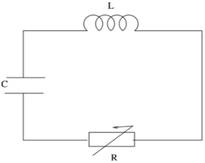
In this section a description of the Van der Pol equation can be expressed[12]. The Van der Pol oscillator is a self-maintained electrical circuit consisted of an inductor (L), a capacitor initially charged with a capacitance (C) and a non-linear resistance (R); all of which are connected in se-ries as indicated in Figure 1. This oscillator was invented by Van der Pol while he was trying to discover a new way to model the oscillations of a self maintained electrical circuit. The character-istic intensity-tension UR of the nonlinear resis-tance (R) is given as:
UR=−R0i0[ i i0 −
1 3(
i i0
)3] (2.1)
where i0 and R0 are the current and the resis-tance of the normalization, respectively. This
Figure 1: Electric circuit modelizing the Van der Pol oscillator in an autonomous regime.
non-linear resistance can be obtained by using the operational amplifier (op-amp). By applying the links law to Figure 1 we have:
UL+UR+UC = 0 (2.2)
whereUL and UC are the tension to the limits of the inductor and capacitor, respectively, and are defined as:
UL=L di
dτ, (2.3)
UC = 1
C ∫
idτ. (2.4)
Substituting (2.1), (2.3) and (2.4) in (2.2), we have:
Ldi
dτ −R0i0[ i i0 −
1 3(
i i0)
3] + 1 C
∫
idτ = 0. (2.5)
Differentiating (2.5) with respect to τ, we have
Ld 2i
dτ2 −R0[1− i2 i2 0
]di
dτ + i
C = 0. (2.6)
Setting
y= i
i0
(2.7)
and
t=ωeτ (2.8)
where ωe= √1LC is an electric pulsation, we get:
d dτ =ωe
d
dt (2.9)
d2 dτ2 =ω
2 e
d2
Substituting (2.9) and (2.10) in (2.6), yields
d2y dt2R0
√ C L(1−y
2)dy
dt +y= 0. (2.11)
By setting µ = R0 √
C
L, Eq.(2.11) takes dimen-sional form as follows
y′′−µ(1−y2)y′+y= 0. (2.12)
where µ is the scalar parameter indicating the strength of the nonlinear damping, and (2.12) is called the Van der Pol equation in the au-tonomous regime. This equation is expressed with the initial conditions as:
y(0) =α, y′(0) =β. (2.13)
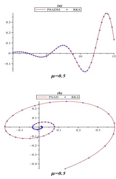
Figure 2: (a): plot of displacementyversus time t; (b): phase plane. Solid line: PSADM; Solid circle: RK4.
Figure 3: (a): plot of displacementyversus time t; (b): phase plane. Solid line: PSADM; Solid circle: RK4.
3
The methodology
3.1 Adomian decomposition method for Van der Pol Equation
The Adomian decomposition method (ADM) is a semi-analytical method for ordinary and partial nonlinear differential equations. The details of this method are presented by G. Adomian[1]. The ADM presented the equation in an operator form by considering the highest-order of derivative in the problem. Hence, in this problem we choose the differential operator L in terms of y′′, then (2.12) can be rewritten in the following form:
Ly=µy′−µy2y′−y, (3.14) where the differential operator Lis
L= d
2
dt2. (3.15)
The inverse operator L−1 is
L−1(.) = ∫ t
0 ∫ t
0
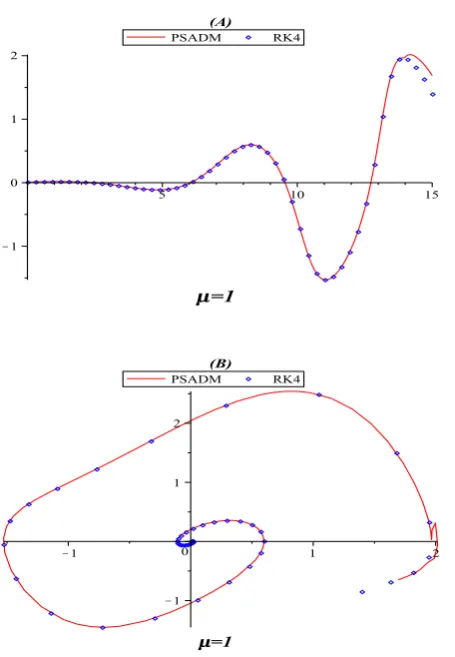
Figure 4: (A): plot of displacementyversus time t; (B): phase plane. Solid line: PSADM; Solid circle: RK4.
Operating withL−1 on (3.14) , it follows
y(t) =y(0)−ty′(0) +µL−1y′(t)
−µL−1y2(t)y′(t)− L−1y(t). (3.17) According to the ADM, the solution y(t) is rep-resented by the decomposition series
y(t) =
∞
∑
n=0
yn(t), (3.18)
and the nonlinear part of Eq. (3.17) is repre-sented by the decomposition series
N(y(t)) =y2(t)y′(t) =
∞
∑
n=0
An(t), (3.19)
where An(t), the Adomian polynomials, are ob-tained as follows:
An= 1
n! dn dλn[N(
n ∑
i=0
λiyi)]λ=0
n= 0,1,2, .... (3.20)
By setting (3.18) and (3.19) in (3.17), we obtain
∞
∑
n=0
yn(t) =y(0)−ty′(0) +µL−1 d dt(
∞
∑
n=0 yn(t))
−µL−1(
∞
∑
n=0
An(t)− L−1(
∞
∑
n=0 yn(t)).
(3.21) To specify the componentsyn(x), ADM wich indi-cates the use of recursive relation will be applied,
y0(t) =y(0)−ty′(0), (3.22)
and
yn+1(t) =µL−1 d
dtyn(t)−µL −1A
n(t)−
L−1y
n(t), n≥0. (3.23) In practice, not all terms of the series in Eq. (3.23) need to be determined and hence, the solu-tion will be approximated by the truncated series
ψk(t) = k−1 ∑
n=0 yn(t)
with
lim
k→∞ψk(t) =y(t). (3.24)
3.2 Chebyshev polynomials
Chebyshev polynomials of the first kind are orthogonal with respect to the weight function
ω(x) = √ 1
1−x2 on the interval[−1,1], and satisfy the following recursive formula:
T0(x) = 1, T1(x) =x, Tn+1(x) = 2xTn(x)−Tn−1(x),
n= 1,2,3, .... (3.25)
This system is orthogonal basis with weight func-tion ω(t) = (1−x2)−1/2 and orthogonality prop-erty:
∫ 1
−1
Tn(x)Tm(x)(1−x2)−1/2dx= π
A functionu(x)∈L2
ω(−1,1) can be expanded by Chebyshev polynomials as follows:
u(x) =
∞ ′
∑
j=0
ujTj(x), (3.27)
where the coefficientsuj are
uj = 2
π < u(x), Tj(x)>ω j= 0,1,2, ....
(3.28)
Here,< ., . >ω is the inner product ofL2ω(−1,1). The grid (interpolation) points are chosen to be the exterma
xi =−cos( iπ
m), i= 0,1, ..., m, (3.29)
of theTm(x). The following approximation of the functionu(x) can be introduced:
u(x)≃u[m](x) = m ∑
j=0
˜
ujTj(x), (3.30)
where ˜uj are the Chebyshev coefficients. These coefficients are determined as follows:
˜
uj =
2(−1)j
mc˜j m ∑
i=0
1 ˜
ci
u(xi) cos( πij
m ),
j=0,1,...,m , (3.31)
where
˜
ci = {
2, i= 0, m
1, 1≤i≤m−1. (3.32)
3.3 Spectral Adomian decomposition method(SADM)
At first, based on initial conditions (2.13), the initial approximation y0(t) = α+βt is selected. By applying iteration formula (3.23), the follow-ing will be obtained
y1(t) =−L−1(A0(t)). (3.33)
From (3.30), the function y1(x) on [0, ξ] can be
approximated as follows:
y1(t)≃y [m] 1 (t) =
m ∑
j=0
˜
y1jTj( 2
ξt−1), (3.34)
where ˜y1j are the Chebyshev coefficients derived from (3.31) as follows:
˜
y1j =
2(−1)j m˜cj
m ∑
i=0
1 ˜
ci
y1(˜ti).cos( πij
m ), j = 0,1, ..., m,
˜
ti = ξ
2(ti+ 1), i= 0, ..., m. (3.35) For finding the unknown coefficients y1(˜ti), i = 0,1, ..., m, by substituting the grid points ˜ti,i= 0,1, ..., m in (3.31), the following will be con-cluded:
y1(˜ti) =−L−1(A0(˜ti)), (3.36)
from (3.35) and (3.36)
˜
y1j =
2(−1)j
m˜cj m ∑
i=0
−1 ˜
ci L
−1(A
0(˜ti)).cos( πij
m ),
j = 0,1, ..., m, (3.37) can be gained. Therefore, from (3.34) and (3.37) the approximation ofy1(t) can be obtained.
For finding the approximation of y2(t) of (3.23),
the following will be gained:
y2(t) =−L−1(A1), (3.38)
in a similar way, the function y2(t) on [0, ξ] can
be approximated as
y2(t)≃y2[m](t) = m ∑
j=0
˜
y2jTj( 2
ξt−1), (3.39)
where
˜
y2j =
2(−1)j
m˜cj m ∑
i=0
1 ˜
ci
y2(˜ti).cos( πij
m ),
j = 0,1, ..., m, (3.40) similarly, for finding the unknown coefficients
y2(˜ti), i = 0,1, ..., m, by substituting the grid points ˜ti, i= 0,1, ..., min (3.38)
can be concluded, therefore, from (3.40) and (3.41)
˜
y2j =
2(−1)j
m˜cj m ∑
i=0
−1 ˜
ci L
−1(A
1(˜ti)).cos( πij
m ),
j= 0,1, ..., m, (3.42) and from (3.39) and (3.42) the approximation of
y2(t) can be obtained.
Generally, for n ≥ 2, according to the above method, the approximation of yn(x) will be achieved as follows:
yn(t)≃yn[m](t) = m ∑
j=0
˜
ynjTj( 2
ξt−1), (3.43)
where
˜
ynj =
2(−1)j
m˜cj m ∑
i=0
−1 ˜
ci L
−1(A
n−1(˜ti)).cos( πij
m ),
j= 0,1, ..., m. (3.44)
At the end,y[0m](t) +y1[m](t) +y2[m](t) +...+yn[m](t) is the (n, m)-term approximation of the series so-lution.
3.4 Piecewise spectral Adomian de-composition method
It is clear that the hybrid spectral Adomian decomposition method is ideally suited for solv-ing differential equations whose solutions do not change rapidly or oscillate over small parts of the domain of the governing problem. For solving strongly-nonlinear oscillators on large domains, we introduce the main idea of the piecewise spec-tral Adomian decomposition method.
We first divide the interval [0, ξ] into subin-tervals Ωr = [ξr−1, ξr] where r = 1, ..., M and ∆r = ξr −ξr−1. Moreover, we define the linear
mappings ψr : Ωr→[−1,1] by
ψr(t) =
2(t−ξr−1)
∆r − 1,
r = 1,2, ..., M, (3.45)
and choose grid points ˜tri as:
˜
tri =ψr−1(ti) = ∆r
2 (ti+ 1) +ξr−1,
r= 1,2, ..., M, i= 0,1, ..., m, (3.46)
where ψ−1
r (ti) is inverse map of ψr(t). On Ω1 =
[ξ0, ξ1], lety1,0(t) =y(ξ0) +y′(ξ0)(t−ξ0) =α+βt
and for k≥1
y1,k(t)≃y1[m,k](t) = m ∑
j=0
˜
y(1)kjTj(ψ1(t)),
(3.47)
where ˜y(1)kj are the Chebyshev coefficients. These coefficients are determined by
˜
y(1)kj = 2(−1) j
m˜cj m ∑ i=0 1 ˜ ci
y1,k(˜t1i).cos( πij
m ),
j= 0,1, ..., m. (3.48)
For finding the unknown coefficients y1,k(˜t1i),i= 0,1, ..., m, by substituting the grid points ˜t1i, i= 0,1, ..., m in (3.31), the following will be con-cluded:
y1,k(˜t1i) =−L−1(A0(˜t1i)), (3.49)
from (3.48) and (3.49)
˜
ykj(1)= 2(−1) j
m˜cj m ∑
i=0
−1 ˜
ci L
−1(A
k−1(˜t1i)).cos( πij
m ),
j = 0,1, ..., m. (3.50)
Now, the (n, m)-term approximation on Ω1 =
[0, ξ1] is introduced as follows:
Φ1[m,n](t) =y1[m,0](t) +y1[m,1](t) +y1[m,2](t) +...
+y[1m,n](t).
(3.51)
Similarly, on Ω2 = [ξ1, ξ2], we have y2,0(t) =
Φ[1m,n](ξ1) + Φ
′[m]
1,n (ξ1)(t−ξ1) and for k≥1,
y2,k(t)≃y2[m,k](t) = m ∑
j=0
˜
y(2)kjTj(ψ2(t)),
(3.52)
where ˜y(2)kj are the Chebyshev coefficients. These coefficients are determined as follows:
˜
y(2)kj = 2(−1) j
m˜cj m ∑ i=0 1 ˜ ci
y2,k(˜t1i).cos( πij
m ),
For finding the unknown coefficients y2,k(˜t2i),i= 0,1, ..., m, by substituting the grid points ˜t2i,i= 0,1, ..., m in (3.31), the following will be con-cluded:
y2,k(˜t2i) =−L−1(A0(˜t2i)), (3.54)
from (3.53) and (3.54)
˜
y(2)kj = 2(−1) j
m˜cj m ∑
i=0
−1 ˜
ci L
−1(A
k−1(˜t2i)).cos( πij
m ),
j = 0,1, ..., m. (3.55)
Now, the (n, m)-term approximation on Ω2 =
[ξ1, ξ2] is introduced as:
Φ2[m,n](t) =y2[m,0](t) +y2[m,1](t) +y2[m,2](t) +...
+y2[m,n](t). (3.56)
In a similar way, we can obtain the (n,m)-order approximation Φ[s,nm](t) =
∑n
k=0ysk(t) on Ωs =
[ξs−1, ξs], s=3,4,...,M. Finally, the approximation solution y(t) in entire interval [0, ξ] is given by
y(t)≃Φ[nm](t) =
Φ[1m,n](t), t∈Ω1,
Φ[2m,n](t), t∈Ω2,
.. .
Φ[M,nm] (t), t∈ΩM, (3.57) where Ω1 = [0, ξ1] , ΩM = [ξM−1, ξ] and Ωs = [ξs−1, ξs] for s = 2,3, ..., M −1. It is clear that [0, ξ] = ∪Ms=1Ωs. According to [13] SADM is convergent on [0, ξ], consequently, it is concluded that PSADM is convergent.
4
Numerical results
According to (2.12) and (2.13), the Van der Pol equation in standard form is as follows:
y′′−µ(1−y2)y′+y= 0, y(0) =α,
y′(0) =β, (4.58)
where µ is a scalar parameter indicating the de-gree of nonlinearity and the strength of the damp-ing. If µ= 0, the equation reduces to the equa-tion of simple harmonic moequa-tion y′′+y = 0. For
µ >0, wheny >1,−µ(1−y2) is positive and the system behaves as a damped (energy dissipating)
system, and when y < 1, −µ(1−y2) is negative
and the system behaves as a self excited (energy absorbing) system.
To demonstrate the validity and applicability of the PSADM, we compare the approximate re-sults given by the presented method in three cases µ = 0.1, µ = 0.5 and µ = 1(∆r = ∆ = 0.5, m = 15, n = 10, M = 30) with numeri-cal solution obtained by 4th order Runge-Kutta method (∆t = 0.001) on interval [0,15]. In all cases, we take α = β = 0.01, and the results are shown in Figures 2, 3 and 4, respectively. From these figures we find that PSADM results are close to the numerical solutions obtained us-ingRK4.
5
Conclusion
In this paper, the piecewise Adomian decompo-sition method was introduced and this method was applied for solving Van der Pol equation, an strongly non-linear and swinging equation. The numerical results presented show that the pro-posed method is a powerful method for solving Van der Pol equation. The advantage of piece-wise spectral Adomin decomposition method over piecewise Adomian decomposition method is that it does not need to calculate complex integrals. Another advantage of the proposed method is that, unlike the spectral method, there is no need to solve algebraic equations (linear or nonlinear). Furthermore, the result obtained from PSADM for Van der Pol equation shows that this method is an accurate and efficient method for solving such equations.
References
[1] G. Adomian, Nonlinear stochastic operator equations, Academic press (2014).
[2] J. H. Cartwright, V. M. Eguiluz, E. Hernandez-Garcia, O. Piro, Dynamics of elastic excitable media, International Journal of Bifurcation and Chaos 9 (1999) 2197-2202.
[4] M. L. Cartwright, Balthazar van der Pol, Journal of the London Mathematical Soci-ety 1 (1960) 367-376.
[5] M. L. Cartwright, J. E. Littlewood,On non-linear equations of the second order: I. The equation Ry k. 1 y2 Py/Py C y D bk cos. t C/; k large, J London Math Soc 20 (1945) 180-189.
[6] A. C. de Pina Filho, M. S. Dutra, Applica-tion of hybrid van der Pol-Rayleigh oscilla-tors for modeling of a bipedal robot, Mechan-ics of Solids in Brazil 1 (2009) 209-221.
[7] E. H. Doha, W. M. Abd-Elhameed, Y. H. Youssri, Second kind Chebyshev opera-tional matrix algorithm for solving differen-tial equations of Lane Emden type, New As-tronomy 23 (2013) 113-117.
[8] R. FitzHugh, Impulses and physiological states in theoretical models of nerve mem-brane, Biophysical journal 1 (1961) 445-452.
[9] D. Gonze, M. Kaufman, Theory of non-linear dynamical systems, Biophysical jour-nal 3 (1961) 1405-1415.
[10] M. Heydari, S. M. Hosseini, G. B. Logh-mani, Numerical Solution of Singular IVPs of Lane-Emden Type Using Integral Oper-ator and Radial Basis Functions, Interna-tional Journal of Industrial Mathematics 4 (2011) 135-146.
[11] H. Y. Hafeez, C. E. Ndikilar, Van der Pol Equation for Nonlinear Plasma Oscillations, Journal of Advanced Physics 3, no. 4 (2014): 278-281.
[12] H. Y. Hafeez, C. E. Ndikilar, S. Isyaku, An-alytical Study of the Van der Pol Equation
in the Autonomous Regime, PROGRESS 11
(2015) 252-262.
[13] S. Gh. Hosseini, S. Abbasbandy, Solution of Lane-Emden Type Equations by Combi-nation of the Spectral Method and Adomian Decomposition Method, Mathematical Prob-lems in Engineering 2015 (2015) 11-22.
[14] N. Levinson, A second order differential equation with singular solutions, Annals of Mathematics 5 (1949) 127-153.
[15] J. Nagumo, S. Arimoto, S. Yoshizawa, An active pulse transmission line simulating nerve axon, Proceedings of the IRE 50, 10 (1962) 2061-2070.
[16] S. Rajasekar, S. Parthasarathy, M. Lak-shmanan. Prediction of horseshoe chaos in BVP and DVP oscillators, Chaos, Solitons and Fractals 3 (1992) 271-280.
[17] M. Tsatsos,Theoretical and Numerical study of the Van der Pol equation, Doctoral deser-tation, Aristotle University of Thessaloniki (2006).
[18] B. Van der Pol, A theory of the amplitude of free and forced triode vibrations, Radio Re-view 1 (1920) 701-710.
Seyed Ghasem Hosseini is Ph.D of applied mathematics . He is mem-ber of Department of mathemat-ics, Ashkezar Branch, Islamic Azad University, Yazd, Iran. His re-search interests include numerical solution of functional equations.
Esmail Babolian is Professor of applied mathematics and Fac-ulty of Mathematical sciences and computer, Kharazmy University, Tehran, Iran. Interested in numer-ical solution of functional Equa-tions, Numerical linear algebra and mathematical education.